Search in book...
Toggle Font Controls
Create new playlist

Name your new playlist

Playlist description (optional)
Sign In

Email address

Password

Forgot Password?

or

Continue with Facebook

Continue with Google
Sign Up

Full Name

Email address

Confirm Email Address

Password

or

Continue with Facebook

Continue with Google

Chapter 2: Using Essential Libraries

There are many production-quality open source C++ libraries and frameworks out there. One of the traits of an experienced graphics developer is their comprehensive knowledge of available open source libraries that are suitable for getting the job done.

In this chapter, we will learn about essential open source libraries and tools that can bring a great productivity boost for you as a developer of graphical applications.

In this chapter, we will cover the following recipes:

Using the GLFW library
Doing math with GLM
Loading images with STB
Rendering a basic UI with Dear ImGui
Integrating EasyProfiler
Integrating Optick
Using the Assimp library
Getting started with Etc2Comp
Multithreading with Taskflow
Introducing MeshOptimizer

Technical requirements

You can find the code files present in this chapter on GitHub at https://github.com/PacktPublishing/3D-Graphics-Rendering-Cookbook/tree/master/Chapter2

Using the GLFW library

The GLFW library hides all the complexity of creating windows, graphics contexts, and surfaces, and getting input events from the operating system. In this recipe, we build a minimalistic application with GLFW and OpenGL to get some basic 3D graphics out onto the screen.

Getting ready

We are building our examples with GLFW 3.3.4. Here is a JSON snippet for the Bootstrap script so that you can download the proper library version:

{

"name": "glfw",

"source": {

"type": "git",

"url": "https://github.com/glfw/glfw.git",

"revision": "3.3.4"

}

The complete source code for this recipe can be found in the source code bundle under the name of Chapter2/01_GLFW.

How to do it...

Let's write a minimal application that creates a window and waits for an exit command from the user. Perform the following steps:

First, we set the GLFW error callback via a simple lambda to catch potential errors:
#include <GLFW/glfw3.h>
...
int main() {
  glfwSetErrorCallback(
     []( int error, const char* description ) {
        fprintf( stderr, "Error: %s ", description );
     });
Now, we can go forward to try to initialize GLFW:
if ( !glfwInit() )
exit(EXIT_FAILURE);
The next step is to tell GLFW which version of OpenGL we want to use. Throughout this book, we will use OpenGL 4.6 Core Profile. You can set it up as follows:
  glfwWindowHint(GLFW_CONTEXT_VERSION_MAJOR, 4);
  glfwWindowHint(GLFW_CONTEXT_VERSION_MINOR, 6);
  glfwWindowHint(    GLFW_OPENGL_PROFILE, GLFW_OPENGL_CORE_PROFILE);
  GLFWwindow* window = glfwCreateWindow(    1024, 768, "Simple example", nullptr, nullptr);
  if (!window) {
    glfwTerminate();
    exit( EXIT_FAILURE );
  }
There is one more thing we need to do before we can focus on the OpenGL initialization and the main loop. Let's set a callback for key events. Again, a simple lambda will do for now:
  glfwSetKeyCallback(window,
    [](GLFWwindow* window,       int key, int scancode, int action, int mods) {
      if ( key == GLFW_KEY_ESCAPE && action ==
          GLFW_PRESS )
             glfwSetWindowShouldClose(               window, GLFW_TRUE );
    });
We should prepare the OpenGL context. Here, we use the GLAD library to import all OpenGL entry points and extensions:
  glfwMakeContextCurrent( window );
  gladLoadGL( glfwGetProcAddress );
  glfwSwapInterval( 1 );

Now we are ready to use OpenGL to get some basic graphics out. Let's draw a colored triangle. To do that, we need a vertex shader and a fragment shader, which are both linked to a shader program, and a vertex array object (VAO). Follow these steps:

First, let's create a VAO. For this example, we will use the vertex shader to generate all vertex data, so an empty VAO will be sufficient:
  GLuint VAO;
  glCreateVertexArrays( 1, &VAO );
  glBindVertexArray( VAO );
To generate vertex data for a colored triangle, our vertex shader should look as follows. Those familiar with previous versions of OpenGL 2.x will notice the layout qualifier with the explicit location value for vec3 color. This value should match the corresponding location value in the fragment shader, as shown in the following code:
static const char* shaderCodeVertex = R"(
#version 460 core
layout (location=0) out vec3 color;
const vec2 pos[3] = vec2[3](
  vec2(-0.6, -0.4),
  vec2(0.6, -0.4),
  vec2(0.0, 0.6)
);
const vec3 col[3] = vec3[3](
vec3(1.0, 0.0, 0.0),
  vec3(0.0, 1.0, 0.0),
  vec3(0.0, 0.0, 1.0)
);
void main() {
  gl_Position = vec4(pos[gl_VertexID], 0.0, 1.0);
  color = col[gl_VertexID];
}
)";
Important note
More details on OpenGL Shading Language (GLSL) layouts can be found in the official Khronos documentation at https://www.khronos.org/opengl/wiki/Layout_Qualifier_(GLSL).
We use the GLSL built-in gl_VertexID input variable to index into the pos[] and col[] arrays to generate the vertex positions and colors programmatically. In this case, no user-defined inputs to the vertex shader are required.
For the purpose of this recipe, the fragment shader is trivial. The location value of 0 of the vec3 color variable should match the corresponding location in the vertex shader:
static const char* shaderCodeFragment = R"(
#version 460 core
layout (location=0) in vec3 color;
layout (location=0) out vec4 out_FragColor;
void main() {
out_FragColor = vec4(color, 1.0);
};
)";
Both shaders should be compiled and linked to a shader program. Here is how we do it:
  const GLuint shaderVertex =    glCreateShader(GL_VERTEX_SHADER);
  glShaderSource(    shaderVertex, 1, &shaderCodeVertex, nullptr);
  glCompileShader(shaderVertex);
  const GLuint shaderFragment =    glCreateShader(GL_FRAGMENT_SHADER);
  glShaderSource(shaderFragment, 1,    &shaderCodeFragment, nullptr);
  glCompileShader(shaderFragment);
  const GLuint program = glCreateProgram();
  glAttachShader(program, shaderVertex);
  glAttachShader(program, shaderFragment);
  glLinkProgram(program);
  glUseProgram(program);
For the sake of brevity, all error checking is omitted in this chapter. We will come back to it in the next Chapter 3, Getting Started with OpenGL and Vulkan.

Now, when all of the preparations are complete, we can jump into the GLFW main loop and examine how our triangle is being rendered.

Let's explore how a typical GLFW application works. Perform the following steps:

The main loop starts by checking whether the window should be closed:
while ( !glfwWindowShouldClose(window) ) {
Implement a resizable window by reading the current width and height from GLFW and updating the OpenGL viewport accordingly:
     int width, height;
     glfwGetFramebufferSize(
       window, &width, &height);
     glViewport(0, 0, width, height);
Important note
Another approach is to set a GLFW window resize callback via glfwSetWindowSizeCallback(). We will use this later on for more complicated examples.
Clear the screen and render the triangle. The glDrawArrays() function can be invoked with the empty VAO that we bound earlier:
     glClearColor(1.0f, 1.0f, 1.0f, 1.0f);
     glClear(GL_COLOR_BUFFER_BIT);
     glDrawArrays(GL_TRIANGLES, 0, 3);
The fragment shader output was rendered into the back buffer. Let's swap the front and back buffers to make the triangle visible. To conclude the main loop, do not forget to poll the events with glfwPollEvents():
     glfwSwapBuffers(window);
     glfwPollEvents();
  }
To make things nice and clean at the end, let's delete the OpenGL objects that we created and terminate GLFW:
  glDeleteProgram(program);
  glDeleteShader(shaderFragment);
  glDeleteShader(shaderVertex);
  glDeleteVertexArrays(1, &VAO);
  glfwDestroyWindow(window);
  glfwTerminate();
  return 0;
}

Here is a screenshot of our tiny application:

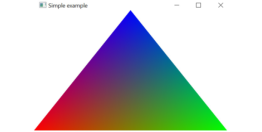
Figure 2.1 – Our first triangle is on the screen

There's more...

The GLFW setup for macOS is quite similar to the Windows operating system. In the CMakeLists.txt file, you should add the following line to the list of used libraries: -framework OpenGL -framework Cocoa -framework CoreView -framework IOKit.

Further details about how to use GLFW can be found at https://www.glfw.org/documentation.html.

Doing math with GLM

Every 3D graphics application needs some sort of math utility functions, such as basic linear algebra or computational geometry. This book uses the OpenGL Mathematics (GLM) header-only C++ mathematics library for graphics, which is based on the GLSL specification. The official documentation (https://glm.g-truc.net) describes GLM as follows:

GLM provides classes and functions designed and implemented with the same naming conventions and functionalities as GLSL so that anyone who knows GLSL, can use GLM as well as C++.

Getting ready

Get the latest version of GLM using the Bootstrap script. We use version 0.9.9.8:

{

"name": "glm",

"source": {

"type": "git",

"url": "https://github.com/g-truc/glm.git",

"revision": "0.9.9.8"

}

Let's make use of some linear algebra and create a more complicated 3D graphics example. There are no lonely triangles this time. The full source code for this recipe can be found in Chapter2/02_GLM.

How to do it...

Let's augment the example from the previous recipe using a simple animation and a 3D cube. The model and projection matrices can be calculated inside the main loop based on the window aspect ratio, as follows:

To rotate the cube, the model matrix is calculated as a rotation around the diagonal (1, 1, 1) axis, and the angle of rotation is based on the current system time returned by glfwGetTime():
const float ratio = width / (float)height;
const mat4 m = glm::rotate( glm::translate(mat4(1.0f), vec3(0.0f, 0.0f, -3.5f)), (float)glfwGetTime(), vec3(1.0f, 1.0f, 1.0f));
const mat4 p = glm::perspective( 45.0f, ratio, 0.1f, 1000.0f);
Now we should pass the matrices into shaders. We use a uniform buffer to do that. First, we need to declare a C++ structure to hold our data:
struct PerFrameData {
mat4 mvp;
int isWireframe;
};
The first field, mvp, will store the premultiplied model-view-projection matrix. The isWireframe field will be used to set the color of the wireframe rendering to make the example more interesting.
The buffer object to hold the data can be allocated as follows. We use the Direct-State-Access (DSA) functions from OpenGL 4.6 instead of the classic bind-to-edit approach:
const GLsizeiptr kBufferSize = sizeof(PerFrameData);
GLuint perFrameDataBuf;
glCreateBuffers(1, &perFrameDataBuf);
glNamedBufferStorage(perFrameDataBuf, kBufferSize, nullptr, GL_DYNAMIC_STORAGE_BIT);
glBindBufferRange(GL_UNIFORM_BUFFER, 0, perFrameDataBuf, 0, kBufferSize);
The GL_DYNAMIC_STORAGE_BIT parameter tells the OpenGL implementation that the content of the data store might be updated after creation through calls to glBufferSubData(). The glBindBufferRange() function binds a range within a buffer object to an indexed buffer target. The buffer is bound to the indexed target of 0. This value should be used in the shader code to read data from the buffer.
In this recipe, we are going to render a 3D cube, so a depth test is required to render the image correctly. Before we jump into the shaders' code and our main loop, we need to enable the depth test and set the polygon offset parameters:
glEnable(GL_DEPTH_TEST);
glEnable(GL_POLYGON_OFFSET_LINE);
glPolygonOffset(-1.0f, -1.0f);
Polygon offset is needed to render a wireframe image of the cube on top of the solid image without Z-fighting. The values of -1.0 will move the wireframe rendering slightly toward the camera.

Let's write the GLSL shaders that are needed for this recipe:

The vertex shader for this recipe will generate cube vertices in a procedural way. This is similar to what we did in the previous triangle recipe. Notice how the PerFrameData input structure in the following vertex shader reflects the PerFrameData structure in the C++ code that was written earlier:
static const char* shaderCodeVertex = R"(
#version 460 core
layout(std140, binding = 0) uniform PerFrameData {
uniform mat4 MVP;
uniform int isWireframe;
};
layout (location=0) out vec3 color;
The positions and colors of cube vertices should be stored in two arrays. We do not use normal vectors here, which means we can perfectly share 8 vertices among all the 6 adjacent faces of the cube:
const vec3 pos[8] = vec3[8](
  vec3(-1.0,-1.0, 1.0), vec3( 1.0,-1.0, 1.0),
  vec3(1.0, 1.0, 1.0), vec3(-1.0, 1.0, 1.0),
   vec3(-1.0,-1.0,-1.0), vec3(1.0,-1.0,-1.0),
  vec3( 1.0, 1.0,-1.0), vec3(-1.0, 1.0,-1.0)
);
const vec3 col[8] = vec3[8](
  vec3(1.0, 0.0, 0.0), vec3(0.0, 1.0, 0.0),
  vec3(0.0, 0.0, 1.0), vec3(1.0, 1.0, 0.0),
   vec3(1.0, 1.0, 0.0), vec3(0.0, 0.0, 1.0),
  vec3(0.0, 1.0, 0.0), vec3(1.0, 0.0, 0.0)
);
Let's use indices to construct the actual cube faces. Each face consists of two triangles:
const int indices[36] = int[36](
  // front   0, 1, 2, 2, 3, 0,
// right 1, 5, 6, 6, 2, 1,
  // back 7, 6, 5, 5, 4, 7,
  // left   4, 0, 3, 3, 7, 4,
  // bottom   4, 5, 1, 1, 0, 4,
  // top   3, 2, 6, 6, 7, 3
);
The main() function of the vertex shader looks similar to the following code block. The gl_VertexID input variable is used to retrieve an index from indices[], which is used to get corresponding values for the position and color. If we are rendering a wireframe pass, set the vertex color to black:
void main() {
  int idx = indices[gl_VertexID];
  gl_Position = MVP * vec4(pos[idx], 1.0);
  color = isWireframe > 0 ? vec3(0.0) : col[idx];
}
)";
The fragment shader is trivial and simply applies the interpolated color:
static const char* shaderCodeFragment = R"(
#version 460 core
layout (location=0) in vec3 color;
layout (location=0) out vec4 out_FragColor;
void main()
{
out_FragColor = vec4(color, 1.0);
};
)";

The only thing we are missing now is how we update the uniform buffer and submit actual draw calls. We update the buffer twice per frame, that is, once per each draw call:

First, we render the solid cube with the polygon mode set to GL_FILL:
PerFrameData perFrameData = { .mvp = p * m, .isWireframe = false };
glNamedBufferSubData( perFrameDataBuf, 0, kBufferSize, &perFrameData);
glPolygonMode(GL_FRONT_AND_BACK, GL_FILL);
glDrawArrays(GL_TRIANGLES, 0, 36);
Then, we update the buffer and render the wireframe cube using the GL_LINE polygon mode and the -1.0 polygon offset that we set up earlier with glPolygonOffset():
perFrameData.isWireframe = true;
glNamedBufferSubData( perFrameDataBuf, 0, kBufferSize, &perFrameData);
glPolygonMode(GL_FRONT_AND_BACK, GL_LINE);
glDrawArrays(GL_TRIANGLES, 0, 36);

The resulting image should look similar to the following screenshot:

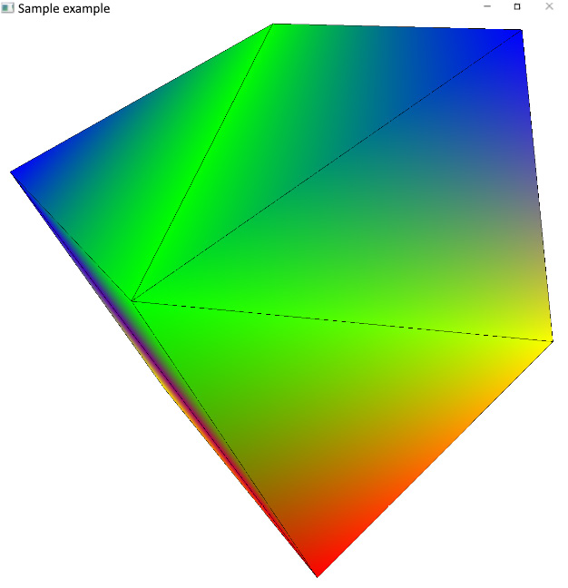
Figure 2.2 – The rotating 3D cube with wireframe contours

There's more...

As you might have noticed in the preceding code, the glBindBufferRange() function takes an offset into the buffer as one of its input parameters. That means we can make the buffer twice as large and store two different copies of PerFrameData in it. One with isWireframe set to true and another one set to false. Then, we can update the entire buffer with just one call to glNamedBufferSubData(), instead of updating the buffer twice, and use the offset parameter of glBindBufferRange() to feed the correct instance of PerFrameData into the shader. This is the correct and most attractive approach, too.

The reason we decided not to use it in this recipe is that the OpenGL implementation might impose alignment restrictions on the value of offset. For example, many implementations require offset to be a multiple of 256. Then, the actual required alignment can be queued as follows:

GLint alignment;

glGetIntegerv( GL_UNIFORM_BUFFER_OFFSET_ALIGNMENT, &alignment);

The alignment requirement would make the simple and straightforward code of this recipe more complicated and difficult to follow without providing any meaningful performance improvements. In more complicated real-world use cases, particularly as the number of different values in the buffer goes up, this approach becomes more useful.

Loading images with STB

Almost every graphics application requires texture images to be loaded from files in some image file formats. Let's take a look at the STB image loader and discuss how we can use it to support popular formats, such as .jpeg, .png, and a floating point format .hdr for high dynamic range texture data.

Getting ready

The STB project consists of multiple header-only libraries. The entire up-to-date package can be downloaded from https://github.com/nothings/stb:

{

"name": "stb",

"source": {

"type": "git",

"url": "https://github.com/nothings/stb.git",

"revision": "c9064e317699d2e495f36ba4f9ac037e88ee371a"

}

The demo source code for this recipe can be found in Chapter2/03_STB.

How to do it...

Let's add texture mapping to the previous recipe. Perform the following steps:

The STB library has separate headers for loading and saving images. Both can be included within your project, as follows:
#define STB_IMAGE_IMPLEMENTATION
#include <stb/stb_image.h>
#define STB_IMAGE_WRITE_IMPLEMENTATION
#include <stb/stb_image_write.h>
To load an image as a 3-channel RGB image from any supported graphics file format, use this short code snippet:
int w, h, comp;
const uint8_t* img = stbi_load( "data/ch2_sample3_STB.jpg", &w, &h, &comp, 3);
Besides that, we can save images into various image file formats. Here is a snippet that enables you to save a screenshot from an OpenGL GLFW application:
int width, height;
glfwGetFramebufferSize(window, &width, &height);
uint8_t* ptr = (uint8_t*)malloc(width * height * 4);
glReadPixels(0, 0, width, height, GL_RGBA, GL_UNSIGNED_BYTE, ptr);
stbi_write_png( "screenshot.png", width, height, 4, ptr, 0);
free(ptr);
Please check stb_image.h and stb_image_write.h for a list of supported file formats.
The loaded img image can be used as an OpenGL texture in a DSA fashion, as follows:
GLuint texture;
glCreateTextures(GL_TEXTURE_2D, 1, &texture);
glTextureParameteri(texture, GL_TEXTURE_MAX_LEVEL, 0);
glTextureParameteri(  texture, GL_TEXTURE_MIN_FILTER, GL_LINEAR);
glTextureParameteri(  texture, GL_TEXTURE_MAG_FILTER, GL_LINEAR);
glTextureStorage2D(texture, 1, GL_RGB8, w, h);
glPixelStorei(GL_UNPACK_ALIGNMENT, 1);
glTextureSubImage2D(texture, 0, 0, 0, w, h, GL_RGB,  GL_UNSIGNED_BYTE, img);
glBindTextures(0, 1, &texture);

Please refer to the source code in Chapter2/03_STB for a complete working example and the GLSL shader changes that are necessary to apply the texture to our cube.

There's more...

STB supports the loading of high-dynamic-range images in Radiance .HDR file format. Use the stbi_loadf() function to load files as floating-point images. This will preserve the full dynamic range of the image and will be useful to load high-dynamic-range light probes for physically-based lighting in the Chapter 6, Physically Based Rendering Using the glTF2 Shading Model.

Rendering a basic UI with Dear ImGui

Graphical applications require some sort of UI. The interactive UI can be used to debug real-time applications and create powerful productivity and visualization tools. Dear ImGui is a fast, portable, API-agnostic immediate-mode GUI library for C++ developed by Omar Cornut (https://github.com/ocornut/imgui):

Dear ImGui is designed to enable fast iterations and to empower programmers to create content creation tools and visualization/debug tools (as opposed to UI for the average end user). It favors simplicity and productivity toward this goal and lacks certain features normally found in more high-level libraries. Dear ImGui is particularly suited to integration in game engines (for tooling), real-time 3D applications, full-screen applications, embedded applications, or any applications on gaming consoles where operating system features can be non-standard.

The ImGui library provides numerous comprehensive examples that explain how to make a GUI renderer for different APIs, including a 700-line code example using OpenGL 3 and GLFW (imgui/examples/imgui_impl_opengl3.cpp). In this recipe, we will demonstrate how to make a minimalistic ImGui renderer in 200 lines of code using OpenGL 4.6. This is not feature-complete, but it can serve as a good starting point for those who want to integrate ImGui into their own modern graphical applications.

Getting ready

Our example is based on ImGui version v1.83. Here is a JSON snippet for our Bootstrap script so that you can download the library:

{

"name": "imgui",

"source": {

"type": "git",

"url": "https://github.com/ocornut/imgui.git",

"revision" : "v1.83"

}

The full source code can be found in Chapter2/04_ImGui.

How to do it...

Let's start by setting up the vertex arrays, buffers, and shaders that are necessary to render our UI. Perform the following steps:

To render geometry data coming from ImGui, we need a VAO with vertex and index buffers. We will use an upper limit of 256 kilobytes for the indices and vertices data:
GLuint VAO;
glCreateVertexArrays(1, &VAO);
GLuint handleVBO;
glCreateBuffers(1, &handleVBO);
glNamedBufferStorage(handleVBO, 256 * 1024, nullptr, GL_DYNAMIC_STORAGE_BIT);
GLuint handleElements;
glCreateBuffers(1, &handleElements);
glNamedBufferStorage(handleElements, 256 * 1024, nullptr, GL_DYNAMIC_STORAGE_BIT);
The geometry data consist of 2D vertex positions, texture coordinates, and RGBA colors, so we should configure the vertex attributes as follows:
glVertexArrayElementBuffer(VAO, handleElements);
glVertexArrayVertexBuffer(  VAO, 0, handleVBO, 0, sizeof(ImDrawVert));
glEnableVertexArrayAttrib(VAO, 0);
glEnableVertexArrayAttrib(VAO, 1);
glEnableVertexArrayAttrib(VAO, 2);
The ImDrawVert structure is a part of ImGui, which is declared as follows:
struct ImDrawVert {
  ImVec2 pos;
  ImVec2 uv;
  ImU32  col;
};
Vertex attributes corresponding to the positions, texture coordinates, and colors are stored in an interleaved format and should be set up like this:
glVertexArrayAttribFormat(  VAO, 0, 2, GL_FLOAT, GL_FALSE,   IM_OFFSETOF(ImDrawVert, pos));
glVertexArrayAttribFormat(  VAO, 1, 2, GL_FLOAT, GL_FALSE,  IM_OFFSETOF(ImDrawVert, uv));
glVertexArrayAttribFormat(  VAO, 2, 4, GL_UNSIGNED_BYTE, GL_TRUE,  IM_OFFSETOF(ImDrawVert, col));
The IM_OFFSETOF() macro is a part of ImGui, too. It is used to calculate the offset of member fields inside the ImDrawVert structure. The macro definition itself is quite verbose and platform-dependent. Please refer to imgui/imgui.h for implementation details.
The final touch to the VAO is to tell OpenGL that every vertex stream should be read from the same buffer bound to the binding point with an index of 0:
glVertexArrayAttribBinding(VAO, 0, 0);
glVertexArrayAttribBinding(VAO, 1, 0);
glVertexArrayAttribBinding(VAO, 2, 0);
glBindVertexArray(VAO);
Now, let's take a quick look at the shaders that are used to render our UI. The vertex shader looks similar to the following code block. The PerFrameData structure in the shader corresponds to the similar structure of the C++ code:
const GLchar* shaderCodeVertex = R"(
  #version 460 core
  layout (location = 0) in vec2 Position;
  layout (location = 1) in vec2 UV;
  layout (location = 2) in vec4 Color;
  layout (std140, binding = 0) uniform PerFrameData
  {
     uniform mat4 MVP;
  };
  out vec2 Frag_UV;
  out vec4 Frag_Color;
  void main()
  {
     Frag_UV = UV;
     Frag_Color = Color;
     gl_Position = MVP * vec4(Position.xy,0,1);
  }
)";
The fragment shader simply modulates the vertex color with a texture. It should appear as follows:
const GLchar* shaderCodeFragment = R"(
  #version 460 core
  in vec2 Frag_UV;
  in vec4 Frag_Color;
  layout (binding = 0) uniform sampler2D Texture;
  layout (location = 0) out vec4 out_Color;
  void main() {
     out_Color = Frag_Color * texture(       Texture, Frag_UV.st);
  }
)";
The vertex and fragment shaders are compiled and linked in a similar way to the Using the GLFW library recipe, so some parts of the code here have been skipped for the sake of brevity. Please refer to the source code bundle for the complete example:
const GLuint handleVertex = glCreateShader(GL_VERTEX_SHADER);...
const GLuint handleFragment = glCreateShader(GL_FRAGMENT_SHADER);...
const GLuint program = glCreateProgram();...
glUseProgram(program);

These were the necessary steps to set up vertex arrays, buffers, and shaders for UI rendering. There are still some initialization steps that need to be done for ImGui itself before we can render anything. Follow these steps:

Let's set up the data structures that are needed to sustain an ImGui context:
ImGui::CreateContext();
ImGuiIO& io = ImGui::GetIO();
Since we are using glDrawElementsBaseVertex() for rendering, which has a vertex offset parameter of baseVertex, we can tell ImGui to output meshes with more than 65535 vertices that can be indexed with 16-bit indices. This is generally good for performance, as it allows you to render the UI with fewer buffer updates:
io.BackendFlags |= ImGuiBackendFlags_RendererHasVtxOffset;
Now, let's build a texture atlas that will be used for font rendering. ImGui will take care of the .ttf font loading and create a font atlas bitmap, which we can use as an OpenGL texture:
ImFontConfig cfg = ImFontConfig();
Tell ImGui that we are going to manage the memory ourselves:
cfg.FontDataOwnedByAtlas = false;
Brighten up the font a little bit (the default value is 1.0f). Brightening up small fonts is a good trick you can use to make them more readable:
Cfg.RasterizerMultiply = 1.5f;
Calculate the pixel height of the font. We take our default window height of 768 and divide it by the desired number of text lines to be fit in the window:
cfg.SizePixels = 768.0f / 32.0f;
Align every glyph to the pixel boundary and rasterize them at a higher quality for sub-pixel positioning. This will improve the appearance of the text on the screen:
cfg.PixelSnapH = true;
cfg.OversampleH = 4;
cfg.OversampleV = 4;
And, finally, load a .ttf font from a file:
ImFont* Font = io.Fonts->AddFontFromFileTTF( "data/OpenSans-Light.ttf", cfg.SizePixels, &cfg);

Now, when the ImGui context initialization is complete, we should take the font atlas bitmap created by ImGui and use it to create an OpenGL texture:

First, let's take the font atlas bitmap data from ImGui in 32-bit RGBA format and upload it to OpenGL:
unsigned char* pixels = nullptr;
int width, height;
io.Fonts->GetTexDataAsRGBA32( &pixels, &width, &height);
The texture creation code should appear as follows:
GLuint texture;
glCreateTextures(GL_TEXTURE_2D, 1, &texture);
glTextureParameteri(texture, GL_TEXTURE_MAX_LEVEL, 0);
glTextureParameteri(  texture, GL_TEXTURE_MIN_FILTER, GL_LINEAR);
glTextureParameteri(  texture, GL_TEXTURE_MAG_FILTER, GL_LINEAR);
glTextureStorage2D(  texture, 1, GL_RGBA8, width, height);
Scanlines in the ImGui bitmap are not padded. Disable the pixel unpack alignment in OpenGL by setting its value to 1 byte to handle this correctly:
glPixelStorei(GL_UNPACK_ALIGNMENT, 1);
glTextureSubImage2D(texture, 0, 0, 0, width, height, GL_RGBA, GL_UNSIGNED_BYTE, pixels);
glBindTextures(0, 1, &texture);
We should pass the texture handle to ImGui so that we can use it in subsequent draw calls when required:
io.Fonts->TexID = (ImTextureID)(intptr_t)texture;
io.FontDefault = Font;
io.DisplayFramebufferScale = ImVec2(1, 1);

Now we are ready to proceed with the OpenGL state setup for rendering. All ImGui graphics should be rendered with blending and the scissor test turned on and the depth test and backface culling disabled. Here is the code snippet to set this state:

glEnable(GL_BLEND);

glBlendEquation(GL_FUNC_ADD);

glBlendFunc(GL_SRC_ALPHA, GL_ONE_MINUS_SRC_ALPHA);

glDisable(GL_CULL_FACE);

glDisable(GL_DEPTH_TEST);

glEnable(GL_SCISSOR_TEST);

Let's go into the main loop and explore, step by step, how to organize the UI rendering workflow:

The main loop starts in a typical GLFW manner, as follows:
while ( !glfwWindowShouldClose(window) ) {
  int width, height;
  glfwGetFramebufferSize(window, &width, &height);
  glViewport(0, 0, width, height);
  glClear(GL_COLOR_BUFFER_BIT);
Tell ImGui our current window dimensions, start a new frame, and render a demo UI window with ShowDemoWindow():
  ImGuiIO& io = ImGui::GetIO();
  io.DisplaySize =    ImVec2( (float)width, (float)height );
  ImGui::NewFrame();
  ImGui::ShowDemoWindow();
The geometry data is generated in the ImGui::Render() function and can be retrieved via ImGui::GetDrawData():
ImGui::Render();
const ImDrawData* draw_data = ImGui::GetDrawData();
Let's construct a proper orthographic projection matrix based on the left, right, top, and bottom clipping planes provided by ImGui:
  Const float L = draw_data->DisplayPos.x;
  const float R = draw_data->DisplayPos.x +                  draw_data->DisplaySize.x;
  const float T = draw_data->DisplayPos.y;
  const float B = draw_data->DisplayPos.y +                  draw_data->DisplaySize.y;
  const mat4 orthoProj = glm::ortho(L, R, B, T);
  glNamedBufferSubData( perFrameDataBuffer, 0,    sizeof(mat4), glm::value_ptr(orthoProj) );
Now we should go through all of the ImGui command lists, update the content of the index and vertex buffers, and invoke the rendering commands:
for (int n = 0; n < draw_data->CmdListsCount; n++) {
const ImDrawList* cmd_list = draw_data->CmdLists[n];
Each ImGui command list has vertex and index data associated with it. Use this data to update the appropriate OpenGL buffers:
glNamedBufferSubData(handleVBO, 0, (GLsizeiptr)cmd_list->VtxBuffer.Size * sizeof(ImDrawVert), cmd_list->VtxBuffer.Data);
glNamedBufferSubData(handleElements, 0, (GLsizeiptr)cmd_list->IdxBuffer.Size * sizeof(ImDrawIdx), cmd_list->IdxBuffer.Data);
Rendering commands are stored inside the command buffer. Iterate over them and render the actual geometry:
     for (int cmd_i = 0; cmd_i < cmd_list->          CmdBuffer.Size; cmd_i++ )      {
        const ImDrawCmd* pcmd =          &cmd_list->CmdBuffer[cmd_i];
        const ImVec4 cr = pcmd->ClipRect;
        glScissor(           (int)cr.x, (int)(height - cr.w),           (int)(cr.z - cr.x), (int)(cr.w - cr.y) );
        glBindTextureUnit(          0, (GLuint)(intptr_t)pcmd->TextureId);
        glDrawElementsBaseVertex(GL_TRIANGLES,          (GLsizei)pcmd->ElemCount, GL_UNSIGNED_SHORT,          (void*)(intptr_t)(pcmd->IdxOffset *          sizeof(ImDrawIdx)), (GLint)pcmd->VtxOffset);
     }
  }
After the UI rendering is complete, reset the scissor rectangle and do the usual GLFW stuff to swap the buffers and poll user events:
  glScissor(0, 0, width, height);
  glfwSwapBuffers(window);
  glfwPollEvents();
}

Once we exit the main loop, we should destroy the ImGui context with ImGui::DestroyContext(). OpenGL object deletion is similar to some of the previous recipes and will be omitted here for the sake of brevity.

The preceding code will render the UI. To enable user interaction, we need to pass user input events from GLWF to ImGui. Let's demonstrate how to deal with the mouse input to make our minimalistic UI interactive:

First, let's install a cursor position callback for GLFW:
glfwSetCursorPosCallback(window,  []( auto* window, double x, double y ) {
     ImGui::GetIO().MousePos = ImVec2(x, y );
  });
The final thing we need to bring our UI to life is to set the mouse button callback and route the mouse button events into ImGui:
glfwSetMouseButtonCallback(window,  [](auto* window, int button, int action, int mods) {
     auto& io = ImGui::GetIO();
     int idx = button == GLFW_MOUSE_BUTTON_LEFT ?        0 : button == GLFW_MOUSE_BUTTON_RIGHT ? 2 : 1;
     io.MouseDown[idx] = action == GLFW_PRESS;
  });

Now we can run our demo application. The application for this recipe renders a Dear ImGui demo window. If everything has been done correctly, the resulting output should look similar to the following screenshot. It is possible to interact with the UI using a mouse:

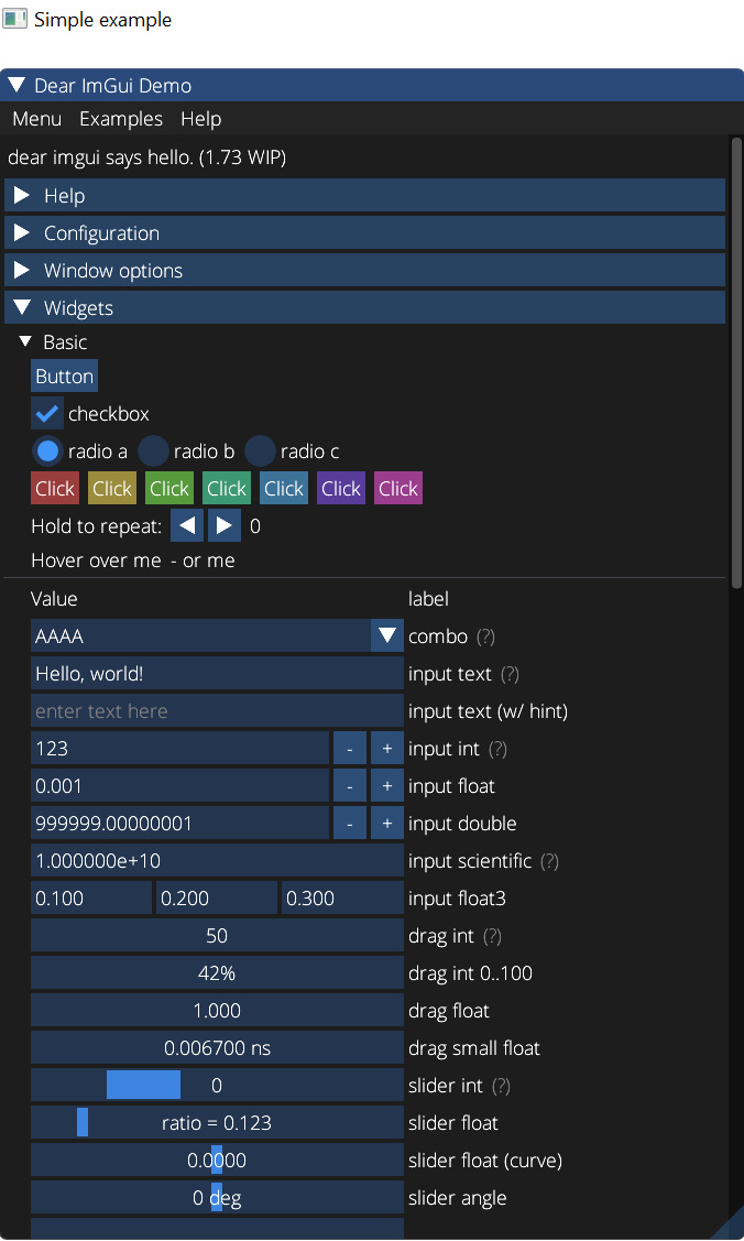
Figure 2.3 – The Dear ImGui demo window

There's more…

Our minimalistic implementation skipped some features that were needed to handle all ImGui rendering possibilities. For example, we did not implement user-defined rendering callbacks or the handling of flipped clipping rectangles. Please refer to imgui/examples/imgui_impl_opengl3.cpp for more details.

Another important part is to pass all of the necessary GLFW events into ImGui, including numerous keyboard events, cursor shapes, scrolling, and more. The complete reference implementation can be found in imgui/examples/imgui_impl_glfw.cpp.

Integrating EasyProfiler

Profiling enables developers to get vital measurement data and feedback in order to optimize the performance of their applications. EasyProfiler is a lightweight cross-platform profiler library for C++, which can be used to profile multithreaded graphical applications (https://github.com/yse/easy_profiler).

Getting ready

Our example is based on EasyProfiler version 2.1. The JSON snippet for Bootstrap to download it looks like this:

{

"name": "easy_profiler",

"source": {

"type": "archive",

"url": "https://github.com/yse/easy_profiler/ releases/download/v2.1.0/ easy_profiler-v2.1.0-msvc15-win64.zip",

"sha1": "d7b99c2b0e18e4c6f963724c0ff3a852a34b1b07"

}

There are two CMake options to set up in CMakeLists.txt so that we can build EasyProfiler without the GUI and demo samples:

set(EASY_PROFILER_NO_GUI ON CACHE BOOL "")

set(EASY_PROFILER_NO_SAMPLES ON CACHE BOOL "")

Now we are good to go and can use it in our application. The full source code for this recipe can be found in Chapter2/05_EasyProfiler.

How to do it...

Let's build a small application that integrates EasyProfiler and outputs a profiling report. Perform the following steps:

First, let's initialize EasyProfiler at the beginning of our main() function:
#include <easy/profiler.h>
...
int main() {
  EASY_MAIN_THREAD;
  EASY_PROFILER_ENABLE;
  ...
Now we can manually mark up blocks of code to be reported by the profiler:
  EASY_BLOCK("Create resources");
  const GLuint shaderVertex =    glCreateShader(GL_VERTEX_SHADER);
  ...
  const GLuint shaderFragment =    glCreateShader(GL_FRAGMENT_SHADER);
  ...
  GLuint perFrameDataBuffer;
  glCreateBuffers(1, &perFrameDataBuffer);
  ...
  EASY_END_BLOCK;
Blocks can be automatically scoped. So, once we exit a C++ scope via }, the block will be automatically ended even if there is no explicit call to EASY_END_BLOCK, as shown in the following snippet:
  {
     EASY_BLOCK("Set state");
     glClearColor(1.0f, 1.0f, 1.0f, 1.0f);
     glEnable(GL_DEPTH_TEST);
     glEnable(GL_POLYGON_OFFSET_LINE);
     glPolygonOffset(-1.0f, -1.0f);
  }
Let's create some nested blocks inside the main loop. We use std::this_thread::sleep_for( std::chrono::milliseconds(2) ) to simulate some heavy computations inside blocks:
  while ( !glfwWindowShouldClose(window) ) {
     EASY_BLOCK("MainLoop");
     ...
     {
        EASY_BLOCK("Pass1");
        std::this_thread::sleep_for(
        std::chrono::milliseconds(2) );
        ...
     }
     {
        EASY_BLOCK("Pass2");
        std::this_thread::sleep_for(
        std::chrono::milliseconds(2) );
        ...
     }
     {
        EASY_BLOCK("glfwSwapBuffers()");
        glfwSwapBuffers(window);
     }
     {
        EASY_BLOCK("glfwPollEvents()");
        std::this_thread::sleep_for(
        std::chrono::milliseconds(2) );
        glfwPollEvents();
     }
  }
At the end of the main loop, we save the profiling data to a file like this:
profiler::dumpBlocksToFile( "profiler_dump.prof" );

Now we can use the GUI tool to inspect the results.

How it works...

On Windows, we use the precompiled version of profiler_gui.exe, which comes with EasyProfiler:

profiler_gui.exe profiler_dump.prof

The output should look similar to the following screenshot:

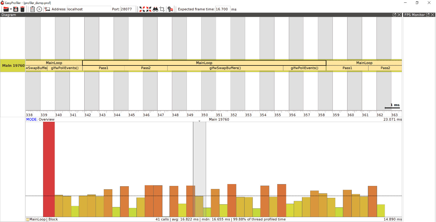
Figure 2.4 – The EasyProfiler GUI

There's more...

Blocks can have different colors, for example, EASY_BLOCK("Block1", profiler::colors::Magenta). Besides that, there is an EASY_FUNCTION() macro that will automatically create a block using the current function name as the block name. Custom ARGB colors can be used in the hexadecimal notation; for example, take a look at the following:

void bar() {

EASY_FUNCTION(0xfff080aa);

}

Integrating Optick

There are numerous profiling libraries for C++ that are useful for 3D graphics development. Some of them are truly generic, such as the one in the previous recipe, while others have specific functionality for profiling graphics applications. There is yet another popular, super-lightweight C++ open source profiler for games, called Optick (https://github.com/bombomby/optick). Besides Windows, Linux, and macOS, it supports Xbox and PlayStation 4 (for certified developers), as well as GPU counters in Direct3D 12 and Vulkan.

Getting ready

We use Optick version 1.3.1, which can be downloaded with the following Bootstrap script:

{

"name": "optick",

"source": {

"type": "git",

"url": "https://github.com/bombomby/optick.git",

"revision": "1.3.1.0"

}

If you want to compile the Optick GUI for Linux or macOS, please refer to the official documentation at https://github.com/bombomby/optick/wiki/How-to-start%3F-(Programmers-Setup). The source code for this recipe can be found in Chapter2/06_Optick.

How to do it...

Integration with Optick is similar to EasyProfiler. Let's go through it step by step:

To start the capture, use the following two macros near the beginning of the main() function:
OPTICK_THREAD("MainThread");
OPTICK_START_CAPTURE();
To mark up blocks for profiling, use the OPTICK_PUSH() and OPTICK_POP() macros, as follows:
{
  OPTICK_PUSH( "Pass1" );
  std::this_thread::sleep_for(
  std::chrono::milliseconds(2) );
  ...
  OPTICK_POP();
}
{
  OPTICK_PUSH( "Pass2" );
  std::this_thread::sleep_for(
  std::chrono::milliseconds(2) );
  ...
  OPTICK_POP();
}
Blocks defined with OPTICK_PUSH() do not close automatically at the scope exit; therefore, an explicit call to OPTICK_POP() is required.
At the end of the main loop, we save the profiling data to a file like this:
OPTICK_STOP_CAPTURE();
OPTICK_SAVE_CAPTURE("profiler_dump");

Now we can compile and run the demo application. The capture data will be saved inside a .opt file with the appended date and time: profiler_dump(2019-11-30.07-34-53).opt. Let's examine what the profiling results look like next.

How it works...

After the demo application exits, run the Optick GUI with the following command to inspect the profiling report:

Optick.exe "profiler_dump(2019-11-30.07-34-53).opt"

The output should be similar to the following screenshot. Each CPU frame can be inspected by clicking on it in the flame graph:

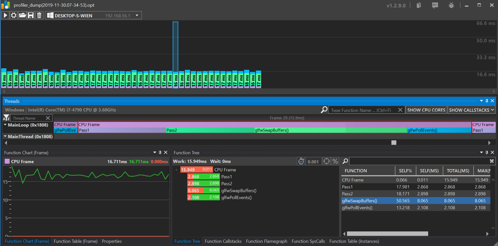
Figure 2.5 – The Optick GUI

Note

Building the Optick GUI for Linux or macOS is not possible since it is written in C# and requires at least the MS VS 2010 CMake generator.

There's more…

Optick provides integration plugins for Unreal Engine 4. For more details, please refer to the documentation at https://github.com/bombomby/optick/wiki/UE4-Optick-Plugin.

At the time of writing this book, building the Optick GUI was only possible on Windows. Therefore, Linux and OS X can only be used for data collection.

Using the Assimp library

Open Asset Import Library, which can be shortened to Assimp, is a portable open source C++ library that can be used to load various popular 3D model formats in a uniform manner.

Getting ready

We will use Assimp version 5.0 for this recipe. Here is the Bootstrap JSON snippet that you can use to download it:

{

"name": "assimp",

"source": {

"type": "git",

"url": "https://github.com/assimp/assimp.git",

"revision": "a9f82dbe0b8a658003f93c7b5108ee4521458a18"

}

Before we can link to Assimp, let's disable the unnecessary functionality in CMakeLists.txt. We will only be using the .obj and .gltf 3D format importers throughout this book:

set(ASSIMP_NO_EXPORT ON CACHE BOOL "")

set(ASSIMP_BUILD_ASSIMP_TOOLS OFF CACHE BOOL "")

set(ASSIMP_BUILD_TESTS OFF CACHE BOOL "")

set(ASSIMP_INSTALL_PDB OFF CACHE BOOL "")

set( ASSIMP_BUILD_ALL_IMPORTERS_BY_DEFAULT OFF CACHE BOOL "")

set(ASSIMP_BUILD_OBJ_IMPORTER ON CACHE BOOL "")

set(ASSIMP_BUILD_GLTF_IMPORTER ON CACHE BOOL "")

The full source code can be found in Chapter2/07_Assimp.

How to do it...

Let's load a 3D model from a .glft2 file via Assimp. The simplest code to do this will look like this:

First, we request the library to convert any geometric primitives it might encounter into triangles:
const aiScene* scene = aiImportFile( "data/rubber_duck/scene.gltf", aiProcess_Triangulate);
Additionally, we do some basic error checking, as follows:
if ( !scene || !scene->HasMeshes() ) {
printf("Unable to load file ");
exit( 255 );
}
Now we can convert the loaded 3D scene into a data format that we can use to upload the model into OpenGL. For this recipe, we will only use vertex positions in vec3 format without indices:
std::vector<vec3> positions;
const aiMesh* mesh = scene->mMeshes[0];
for (unsigned int i = 0; i != mesh->mNumFaces; i++) {
const aiFace& face = mesh->mFaces[i];
const unsigned int idx[3] = { face.mIndices[0], face.mIndices[1], face.mIndices[2] };
To keep this example as simple as possible, we can flatten all of the indices and store only the vertex positions. Swap the y and z coordinates to orient the model:
  for (int j = 0; j != 3; j++) {
     const aiVector3D v = mesh->mVertices[idx[j]];
     positions.push_back( vec3(v.x, v.z, v.y) );
  }
}
Now we can deallocate the scene pointer with aiReleaseImport(scene) and upload the content of positions[] into an OpenGL buffer:
GLuint VAO;
glCreateVertexArrays(1, &VAO);
glBindVertexArray(VAO);
GLuint meshData;
glCreateBuffers(1, &meshData);
glNamedBufferStorage(meshData,  sizeof(vec3) * positions.size(), positions.data(), 0);
glVertexArrayVertexBuffer(  VAO, 0, meshData, 0, sizeof(vec3) );
glEnableVertexArrayAttrib(VAO, 0 );
glVertexArrayAttribFormat(  VAO, 0, 3, GL_FLOAT, GL_FALSE, 0);
glVertexArrayAttribBinding(VAO, 0, 0);
Save the number of vertices to be used by glDrawArrays() in the main loop and render the 3D model:
const int numVertices = static_cast<int>(positions.size());

Here, we use the same two-pass technique from the Doing math with GLM recipe to render a wireframe 3D model on top of a solid image:

while ( !glfwWindowShouldClose(window) ) {

...

glPolygonMode(GL_FRONT_AND_BACK, GL_FILL);

glDrawArrays(GL_TRIANGLES, 0, numVertices);

...

glPolygonMode(GL_FRONT_AND_BACK, GL_LINE);

glDrawArrays(GL_TRIANGLES, 0, numVertices);

glfwSwapBuffers(window);

glfwPollEvents();

}

The output graphics should look similar to the following screenshot:

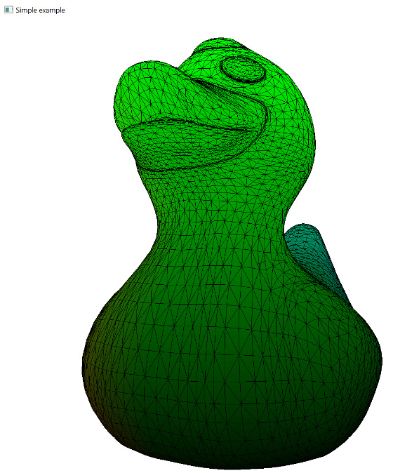
Figure 2.6 – A wireframe rubber duck

Getting started with Etc2Comp

One significant drawback of high-resolution textured data is that it requires a lot of GPU memory to store and process. All modern, real-time rendering APIs provide some sort of texture compression, allowing us to store textures in compressed formats on the GPU. One such format is ETC2. This is a standard texture compression format for OpenGL and Vulkan.

Etc2Comp is an open source tool that converts bitmaps into ETC2 format. The tool is built with a focus on encoding performance to reduce the amount of time required to package asset-heavy applications and reduce the overall application size. In this recipe, you will learn how to integrate this tool within your own applications to construct tools for your custom graphics preparation pipelines.

Getting ready

The project can be downloaded using this Bootstrap snippet:

{

"name": "etc2comp",

"source": {

"type": "git",

"url": "https://github.com/google/etc2comp",

"revision": "9cd0f9cae0f32338943699bb418107db61bb66f2"

}

Etc2Comp was released by Google "as-is" with the intention of being used as a command-line tool. Therefore, we will need to include some additional .cpp files within the CMake target to use it as a library that is linked to our application. The Chapter2/08_ETC2Comp/CMakeLists.txt file contains the following lines to do this:

target_sources(Ch2_Sample08_ETC2Comp PUBLIC ${CMAKE_CURRENT_BINARY_DIR}/../../../ deps/src/etc2comp/EtcTool/EtcFile.cpp)

target_sources(Ch2_Sample08_ETC2Comp PUBLIC ${CMAKE_CURRENT_BINARY_DIR}/../../../ deps/src/etc2comp/EtcTool/EtcFileHeader.cpp)

The complete source code is located at Chapter2/08_ETC2Comp.

How to do it...

Let's build an application that loads a .jpg image via the STB library, converts it into an ETC2 image, and saves it within the .ktx file format:

First, it is necessary to include some header files:
#include "etc2comp/EtcLib/Etc/Etc.h"
#include "etc2comp/EtcLib/Etc/EtcImage.h"
#include "etc2comp/EtcLib/Etc/EtcFilter.h"
#include "etc2comp/EtcTool/EtcFile.h"
#define STB_IMAGE_IMPLEMENTATION
#include <stb/stb_image.h>
Let's load an image as a 4-component RGBA bitmap:
int main() {
int w, h, comp;
const uint8_t* img = stbi_load( "data/ch2_sample3_STB.jpg", &w, &h, &comp, 4);
Etc2Comp takes floating-point RGBA bitmaps as input, so we have to convert our data, as follows:
  std::vector<float> rgbaf;
  for (int i = 0; i != w * h * 4; i+=4) {
     rgbaf.push_back(img[i+0] / 255.0f);
     rgbaf.push_back(img[i+1] / 255.0f);
     rgbaf.push_back(img[i+2] / 255.0f);
     rgbaf.push_back(img[i+3] / 255.0f);
  }
Note
Besides manual conversion, as mentioned earlier, STB can load 8-bit-per-channel images as floating-point images directly via the stbi_loadf() API. However, it will do an automatic gamma correction. Use stbi_ldr_to_hdr_scale(1.0f) and stbi_ldr_to_hdr_gamma(2.2f) if you want to control the amount of gamma correction.
Now we can encode the floating-point image into ETC2 format using Etc2Comp. Because we don't use alpha transparency, our target format should be RGB8. We will use the default BT.709 error metric minimization schema:
  const auto etcFormat = Etc::Image::Format::RGB8;
  const auto errorMetric = Etc::ErrorMetric::BT709;
  Etc::Image image(rgbaf.data(), w, h, errorMetric);
The encoder takes the number of threads as input. Let's use the value returned by thread::hardware_concurrency() and 1024 as the number of concurrent jobs:
  image.Encode(etcFormat, errorMetric,    ETCCOMP_DEFAULT_EFFORT_LEVEL,    std::thread::hardware_concurrency(), 1024);
Once the image is converted, we can save it into the .ktx file format, which can store compressed texture data that is directly consumable by OpenGL. Etc2Comp provides the Etc::File helper class to do this:
  Etc::File etcFile("image.ktx",    Etc::File::Format::KTX,    etcFormat,    image.GetEncodingBits(),   image.GetEncodingBitsBytes(),   image.GetSourceWidth(),    image.GetSourceHeight(),    image.GetExtendedWidth(),    image.GetExtendedHeight());
  etcFile.Write();
  return 0;
}

The bitmap is saved within the image.ktx file. It can be loaded into an OpenGL or Vulkan texture, which we will do in subsequent chapters.

There's more...

Pico Pixel is a great tool that you can use to view .ktx files and other texture formats (https://pixelandpolygon.com). It is freeware but not open source. There is an issues tracker that is publicly available on GitHub. You can find it at https://github.com/inalogic/pico-pixel-public/issues.

For those who want to jump into the latest state-of-the-art texture compression techniques, please refer to the Basis project from Binomial at https://github.com/BinomialLLC/basis_universal.

Multithreading with Taskflow

Modern graphical applications require us to harness the power of multiple CPUs to be performant. Taskflow is a fast C++ header-only library that can help you write parallel programs with complex task dependencies quickly. This library is extremely useful as it allows you to jump into the development of multithreaded graphical applications that make use of advanced rendering concepts, such as frame graphs and multithreaded command buffers generation.

Getting ready

Here, we use Taskflow version 3.1.0. You can download it using the following Bootstrap snippet:

{

"name": "taskflow",

"source": {

"type": "git",

"url": "https://github.com/taskflow/taskflow.git",

"revision": "v3.1.0"

}

To debug dependency graphs produced by Taskflow, it is recommended that you install the GraphViz tool from https://www.graphviz.org.

The complete source code for this recipe can be found in Chapter2/09_Taskflow.

How to do it...

Let's create and run a set of concurrent dependent tasks via the for_each() algorithm. Each task will print a single value from an array in a concurrent fashion. The processing order can vary between different runs of the program:

Include the taskflow.hpp header file:
#include <taskflow/taskflow.hpp>
using namespace std;
int main() {
The tf::Taskflow class is the main place to create a task dependency graph. Declare an instance and a data vector to process:
tf::Taskflow taskflow;
std::vector<int> items{ 1, 2, 3, 4, 5, 6, 7, 8 };
The for_each() member function returns a task that implements a parallel-for loop algorithm. The task can be used for synchronization purposes:
auto task = taskflow.for_each( items.begin(), items.end(), [](int item) { std::cout << item; } );
Let's attach some work before and after the parallel-for task so that we can view Start and End messages in the output. Let's call the new S and T tasks accordingly:
taskflow.emplace( []() { std::cout << " S - Start "; }).name("S").precede(task);
taskflow.emplace( []() { std::cout << " T - End "; }).name("T").succeed(task);
Save the generated tasks dependency graph in .dot format so that we can process it later with the GraphViz dot tool:
std::ofstream os("taskflow.dot");
taskflow.dump(os);
Now we can create an executor object and run the constructed taskflow graph:
  Tf::Executor executor;
  executor.run(taskflow).wait();
  return 0;
}

One important part to mention here is that the dependency graph can only be constructed once. Then, it can be reused in every frame to run concurrent tasks efficiently.

The output from the preceding program should look similar to the following listing:

S - Start

39172 runs 6

46424 runs 5

17900 runs 2

26932 runs 1

26932 runs 8

23888 runs 3

45464 runs 7

32064 runs 4

T - End

Here, we can see our S and T tasks. Between them, there are multiple threads with different IDs processing different elements of the items[] vector in parallel.

There's more...

The application saved the dependency graph inside the taskflow.dot file. It can be converted into a visual representation by GraphViz using the following command:

dot -Tpng taskflow.dot > output.png

The resulting .png image should look similar to the following screenshot:

Figure 2.7 – The Taskflow dependency graph for for_each()

This functionality is extremely useful when you are debugging complex dependency graphs (and producing complex-looking images for your books and papers).

The Taskflow library functionality is vast and provides implementations for numerous parallel algorithms and profiling capabilities. Please refer to the official documentation for in-depth coverage at https://taskflow.github.io/taskflow/index.html.

Introducing MeshOptimizer

For GPUs to render a mesh efficiently, all vertices in the vertex buffer should be unique and without duplicates. Solving this problem efficiently can be a complicated and computationally intensive task in any modern 3D content pipeline.

MeshOptimizer is an open source C++ library developed by Arseny Kapoulkine, which provides algorithms to help optimize meshes for modern GPU vertex and index processing pipelines. It can reindex an existing index buffer or generate an entirely new set of indices from an unindexed vertex buffer.

Getting ready

We use MeshOptimizer version 0.16. Here is the Bootstrap snippet that you can use to download this version:

{

"name": "meshoptimizer",

"source": {

"type": "git",

"url": "https://github.com/zeux/meshoptimizer",

"revision": "v0.16"

}

The complete source code for this recipe can be found in Chapter2/10_MeshOptimizer.

How to do it...

Let's use MeshOptimizer to optimize the vertex and index buffer layouts of a mesh loaded by the Assimp library. Then, we can generate a simplified model of the mesh:

First, we load our mesh via Assimp, as shown in the following code snippet. We preserve the existing vertices and indices exactly as they were loaded by Assimp:
const aiScene* scene = aiImportFile(  "data/rubber_duck/scene.gltf",  aiProcess_Triangulate);
const aiMesh* mesh = scene->mMeshes[0];
std::vector<vec3> positions;
std::vector<unsigned int> indices;
for (unsigned i = 0; i != mesh->mNumVertices; i++) {
  const aiVector3D v = mesh->mVertices[i];
  positions.push_back( vec3(v.x, v.z, v.y) );
}
for (unsigned i = 0; i != mesh->mNumFaces; i++) {
  for ( unsigned j = 0; j != 3; j++ )
     indices.push_back(mesh->mFaces[i].mIndices[j]);
}
aiReleaseImport(scene);
Now we should generate a remap table for our existing vertex and index data:
std::vector<unsigned int> remap( indices.size() );
const size_t vertexCount = meshopt_generateVertexRemap( remap.data(), indices.data(), indices.size(), positions.data(), indices.size(), sizeof(vec3) );
The MeshOptimizer documentation (https://github.com/zeux/meshoptimizer) tells us the following:
The remap table is generated based on binary equivalence of the input vertices, so the resulting mesh will be rendered in the same way.
The returned vertexCount value corresponds to the number of unique vertices that have remained after remapping. Let's allocate space and generate new vertex and index buffers:
std::vector<unsigned int> remappedIndices(  indices.size() );
std::vector<vec3> remappedVertices( vertexCount );
meshopt_remapIndexBuffer( remappedIndices.data(),  indices.data(), indices.size(), remap.data() );
meshopt_remapVertexBuffer( remappedVertices.data(), positions.data(), positions.size(), sizeof(vec3),  remap.data() );
Now we can use other MeshOptimizer algorithms to optimize these buffers even further. The official documentation is pretty straightforward. We will adapt the example it provides for the purposes of our demo application.
When we want to render a mesh, the GPU has to transform each vertex via a vertex shader. GPUs can reuse transformed vertices by means of a small built-in cache, usually storing between 16 and 32 vertices inside it. In order to use this small cache effectively, we need to reorder the triangles to maximize the locality of vertex references. How to do this with MeshOptimizer in place is shown next. Pay attention to how only the indices data is being touched here:
meshopt_optimizeVertexCache( remappedIndices.data(), remappedIndices.data(), indices.size(), vertexCount );
Transformed vertices form triangles that are sent for rasterization to generate fragments. Usually, each fragment is run through a depth test first, and fragments that pass the depth test get the fragment shader executed to compute the final color. As fragment shaders get more and more expensive, it becomes increasingly important to reduce the number of fragment shader invocations. This can be achieved by reducing pixel overdraw in a mesh, and, in general, it requires the use of view-dependent algorithms. However, MeshOptimizer implements heuristics to reorder the triangles and minimize overdraw from all directions. We can use it as follows:
meshopt_optimizeOverdraw( remappedIndices.data(), remappedIndices.data(), indices.size(), glm::value_ptr(remappedVertices[0]), vertexCount, sizeof(vec3), 1.05f );
The last parameter, 1.05, is the threshold that determines how much the algorithm can compromise the vertex cache hit ratio. We use the recommended default value from the documentation.
Once we have optimized the mesh to reduce pixel overdraw, the vertex buffer access pattern can still be optimized for memory efficiency. The GPU has to fetch specified vertex attributes from the vertex buffer and pass this data into the vertex shader. To speed up this fetch, a memory cache is used, which means optimizing the locality of vertex buffer access is very important. We can use MeshOptimizer to optimize our index and vertex buffers for vertex fetch efficiency, as follows:
meshopt_optimizeVertexFetch( remappedVertices.data(), remappedIndices.data(), indices.size(), remappedVertices.data(), vertexCount, sizeof(vec3) );
This function will reorder vertices in the vertex buffer and regenerate indices to match the new contents of the vertex buffer.
The last thing we will do in this recipe is simplify the mesh. MeshOptimizer can generate a new index buffer that uses existing vertices from the vertex buffer with a reduced number of triangles. This new index buffer can be used to render Level-of-Detail (LOD) meshes. The following code snippet shows you how to do this using the default threshold and target error values:
const float threshold = 0.2f;
const size_t target_index_count = size_t( remappedIndices.size() * threshold);
const float target_error = 1e-2f;
std::vector<unsigned int> indicesLod( remappedIndices.size() );
indicesLod.resize( meshopt_simplify( &indicesLod[0], remappedIndices.data(), remappedIndices.size(), &remappedVertices[0].x, vertexCount, sizeof(vec3), target_index_count, target_error) );

Multiple LOD meshes can be generated this way by changing the threshold value.

Let's render the optimized and LOD meshes that we created earlier:

For the simplicity of this demo, we copy the remapped data back into the original vectors as follows:
indices = remappedIndices;
positions = remappedVertices;
With modern OpenGL, we can store vertex and index data inside a single buffer. You can do this as follows:
const size_t sizeIndices =  sizeof(unsigned int) * indices.size();
const size_t sizeIndicesLod =  sizeof(unsigned int) * indicesLod.size();
const size_t sizeVertices =  sizeof(vec3) * positions.size();
glNamedBufferStorage(meshData,  sizeIndices + sizeIndicesLod + sizeVertices,  nullptr, GL_DYNAMIC_STORAGE_BIT);
glNamedBufferSubData(  meshData, 0, sizeIndices, indices.data());
glNamedBufferSubData(meshData, sizeIndices,  sizeIndicesLod, indicesLod.data());
glNamedBufferSubData(meshData, sizeIndices +  sizeIndicesLod, sizeVertices, positions.data());
Now we should tell OpenGL where to read the vertex and index data from. The starting offset to the vertex data is sizeIndices + sizeIndicesLod:
glVertexArrayElementBuffer(VAO, meshData);
glVertexArrayVertexBuffer(VAO, 0, meshData, sizeIndices + sizeIndicesLod, sizeof(vec3));
glEnableVertexArrayAttrib(VAO, 0);
glVertexArrayAttribFormat( VAO, 0, 3, GL_FLOAT, GL_FALSE, 0);
glVertexArrayAttribBinding(VAO, 0, 0);
To render the optimized mesh, we can call glDrawElements(), as follows:
glDrawElements(GL_TRIANGLES, indices.size(), GL_UNSIGNED_INT, nullptr);
To render the simplified LOD mesh, we use the number of indices in the LOD and use an offset to where its indices start in the index buffer. We need to skip sizeIndices bytes to do it:
glDrawElements(GL_TRIANGLES, indicesLod.size(), GL_UNSIGNED_INT, (void*)sizeIndices);

The resulting image should look similar to the following screenshot:

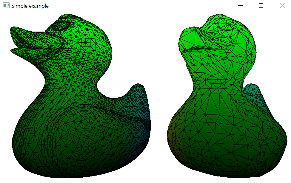
Figure 2.8 – LOD mesh rendering

There's more...

This recipe uses a slightly different technique for the wireframe rendering. Instead of rendering a mesh twice, we use barycentric coordinates to identify the proximity of the triangle edge inside each triangle and change the color accordingly. Here is the geometry shader to generate barycentric coordinates for a triangular mesh:

#version 460 core

layout( triangles ) in;

layout( triangle_strip, max_vertices = 3 ) out;

layout (location=0) in vec3 color[];

layout (location=0) out vec3 colors;

layout (location=1) out vec3 barycoords;

void main()

{

Next, store the values of the barycentric coordinates for each vertex of the triangle:

const vec3 bc[3] = vec3[](

vec3(1.0, 0.0, 0.0),

vec3(0.0, 1.0, 0.0),

vec3(0.0, 0.0, 1.0)

);

for ( int i = 0; i < 3; i++ )

{

gl_Position = gl_in[i].gl_Position;

colors = color[i];

barycoords = bc[i];

EmitVertex();

}

EndPrimitive();

}

Barycentric coordinates can be used inside the fragment shader to discriminate colors in the following way:

#version 460 core

layout (location=0) in vec3 colors;

layout (location=1) in vec3 barycoords;

layout (location=0) out vec4 out_FragColor;

float edgeFactor(float thickness)

{

vec3 a3 = smoothstep( vec3(0.0), fwidth(barycoords) * thickness,barycoords );

return min( min(a3.x, a3.y), a3.z );

}

void main()

{

out_FragColor = vec4(mix(vec3(0.0), colors, edgeFactor(1.0)), 1.0);

};

The fwidth() function calculates the sum of the absolute values of the derivatives in the x and y screen coordinates and is used to determine the thickness of the lines. The smoothstep() function is used for antialiasing.

..................Content has been hidden....................

You can't read the all page of ebook, please click here login for view all page.

Table of Contents for Chapter 2: Using Essential Libraries

Create new playlist

Sign In

Sign Up

Chapter 2: Using Essential Libraries

Technical requirements

Using the GLFW library

Getting ready

How to do it...

There's more...

Doing math with GLM

Getting ready

How to do it...

There's more...

Loading images with STB

Getting ready

How to do it...

There's more...

Rendering a basic UI with Dear ImGui

Getting ready

How to do it...

There's more…

Integrating EasyProfiler

Getting ready

How to do it...

How it works...

There's more...

Integrating Optick

Getting ready

How to do it...

How it works...

There's more…

Using the Assimp library

Getting ready

How to do it...

Getting started with Etc2Comp

Getting ready

How to do it...

There's more...

Multithreading with Taskflow

Getting ready

How to do it...

There's more...

Introducing MeshOptimizer

Getting ready

How to do it...

There's more...

Table of Contents for
Chapter 2: Using Essential Libraries