B
Chaos and Vagueness
There are “simple” systems whose parts are governed by well‐understood physical laws, yet these systems behave unpredictably. If vagueness is indeed a fundamental property of this world, then what is its role in this unpredictable behavior?
B.1 Chaos Theory in a Nutshell
It is a fact that weather forecasting is not easy. It is also known that we cannot predict how the weather will be in 10 or 20 days from now. What is not widely known is why this happens. Moreover, it is not known whether we can make our predictions more accurate and if we can predict the weather for long periods.
Edward Norton Lorenz [195] was a mathematician and meteorologist who wanted to use computers to predict the weather. He created a simple model, but soon he realized that when he slightly changed the input parameters, he was getting completely different results. For example, he noticed that, when his computer simulation was fed with decimal numbers having three decimal digits instead of decimal numbers with six decimal digits, the results were not the same as he would expect. One does not need to reimplement his simulation, which involved 12 ordinary differential equations, instead, one can observe the same effect using a much simpler mathematical expression. For example, one can use an iteration of the quadratic expression ![]() with initial value
with initial value ![]() and
and ![]() . If, at some point, the iteration stops and
. If, at some point, the iteration stops and ![]() is truncated to three decimal digits and the operation resumes with this value and goes to the end without any other interruption, the result will be quite different from what we will get if no interruption happened. This effect, that is known in the literature as the sensitive dependence on initial conditions effect, is a manifestation of a chaotic system. The theory that studies such phenomena is known as chaos theory (see Ref. [239] for an accessible overview).
is truncated to three decimal digits and the operation resumes with this value and goes to the end without any other interruption, the result will be quite different from what we will get if no interruption happened. This effect, that is known in the literature as the sensitive dependence on initial conditions effect, is a manifestation of a chaotic system. The theory that studies such phenomena is known as chaos theory (see Ref. [239] for an accessible overview).
Recently, in a study [34], it was discovered that there are systematic distortions in the statistical properties of chaotic dynamical systems when represented and simulated on digital computers using standard IEEE floating‐point numbers (i.e. the most common representation for real numbers on computers today). However, this is not a limitation of modern computers or modern programming languages, but a limitation imposed by people who implement their simulations using this specific approach. In fact, modern programming languages such as Java and Perl support arbitrary precision decimal numbers that can be used to compute anything to any accuracy. Of course, the calculations are much slower, but this is the price one has to pay when not using IEEE floating‐point numbers.
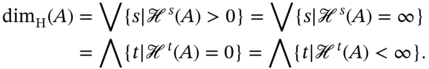
Chaos theory is usually studied alongside fractal geometry (again, see Ref. [239] for an accessible overview of fractal geometry). Fractals are geometric figures, where each part of such a figure looks like the whole figure. This property is known as self‐similarity. In general, objects encountered in Nature do not have the precise properties of the objects of Euclidean geometry. Nevertheless, they can be “approached” by fractals. In a layman's terms, the word dimension is associated with the numbers 1, 2, or 3 if we are talking about points, plane objects, or solid objects, respectively. However, each fractal object has its own fractal dimension, which is a rational or, more generally, a real number. Most of the time, when we say fractal dimension, we actually mean Hausdorff dimension.1
The Hausdorff dimension ![]() of a subset
of a subset ![]() is then defined as
is then defined as
In order to give a formal definition of fractals, we need to be familiar with the notion of topological dimension (also known as Lebesgue covering dimension) [118].
Using these notions, Benoit B. Mandelbrot [209], the father of fractal geometry, gave the following definition:
In addition, every set with an noninteger ![]() is a fractal.
is a fractal.
Unfortunately, the definition of the Hausdorff dimension is such that it is causing difficulty to calculate on computers. Thus, we typically use the capacity dimension that can be computed with the box‐counting algorithm. The description of the algorithm that follows is based on its presentation in [128].
Suppose the space is such that one can define sensible distances and its integer dimension is ![]() . In this space, we are able to cover a fractal with
. In this space, we are able to cover a fractal with ![]() ‐dimensional boxes (i.e. squares, cubes, etc.). Their sizes are regulated by one dimensionless parameter
‐dimensional boxes (i.e. squares, cubes, etc.). Their sizes are regulated by one dimensionless parameter ![]() . This is always possible by choosing nondimensionless basic units so that
. This is always possible by choosing nondimensionless basic units so that ![]() becomes just a scaling factor. Next, we count the number
becomes just a scaling factor. Next, we count the number ![]() of boxes that cover some part of the fractal.
of boxes that cover some part of the fractal. ![]() is connected to the capacity or box‐counting dimension,
is connected to the capacity or box‐counting dimension, ![]() , by
, by
By plotting ![]() against
against ![]() for many values of
for many values of ![]() , we get a straight line whose slope is the fractal dimension. When the resulting curve is not a straight line, we employ the least square method to compute an approximation of the fractal dimension.
, we get a straight line whose slope is the fractal dimension. When the resulting curve is not a straight line, we employ the least square method to compute an approximation of the fractal dimension.
B.2 Fuzzy Chaos
A form of fuzzy chaos was proposed by Oscar Castillo and Patricia Melin [60]. Their starting point is dynamical systems that can be expressed as a nonlinear differential equation:
Or as a nonlinear difference equation:
In order to define and then to study fuzzy chaos, the authors considered a dynamical system on the real line given as follows:
The idea is to associate chaotic behavior with the number of period doublings (or bifurcations, that is, a separation of a structure into two branches) that occur when the parameter ![]() is varied.
is varied.
An alternative definition that relies on fractal dimensions follows:
As was explained earlier, a numerical simulation of a dynamical system is realized by a feedback process, where the output produced by a function at some stage ![]() is given as input to the same function at stage
is given as input to the same function at stage ![]() . The output generated by such a simulation is called a time series:
. The output generated by such a simulation is called a time series: ![]() ,
, ![]() ,…,
,…, ![]() . Next, we need to make a behavior identification for the dynamic system. For example, we can define the typical dynamic behaviors of a three‐dimensional system with the following fuzzy rules:
. Next, we need to make a behavior identification for the dynamic system. For example, we can define the typical dynamic behaviors of a three‐dimensional system with the following fuzzy rules:
| If fractal dimension is low, | Then behavior is cycle of period 2. |
| If fractal dimension is small, | Then behavior is cycle of period 4. |
| If fractal dimension is regular, | Then behavior is cycle period 8. |
| If fractal dimension is medium, | Then behavior is cycle period 16. |
| If fractal dimension is high, | Then behavior is high order cycles. |
| If fractal dimension is large, | Then behavior is fuzzy chaos. |
Here the fractal dimension can be calculated using the box‐counting algorithm and the time series. In addition, the fractal dimension and the behavior are linguistic variables and one needs to define their membership functions.
Now, let us consider a dynamic system that is described by the following mathematical model:
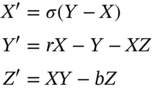
Here ![]() and
and ![]() ,
, ![]() , and
, and ![]() are positive numbers. However, there is a problem here: How do we choose these parameters? Fortunately, there is an algorithm that can be used to choose the best set of parameters. This algorithm is presented in Figure B.1. Also, the genetic algorithm mentioned in Figure B.1 is presented in Figure B.2.
are positive numbers. However, there is a problem here: How do we choose these parameters? Fortunately, there is an algorithm that can be used to choose the best set of parameters. This algorithm is presented in Figure B.1. Also, the genetic algorithm mentioned in Figure B.1 is presented in Figure B.2.
| Step 1 | Read the mathematical model |
| Step 2 | Analyze the model |
| Step 3 | Generate a set of admissible parameters using the understanding of the model. |
| Step 4 | Choose the best set of parameter values using a specific genetic algorithm. |
| Step 5 | Perform the simulations by solving numerically the equations of the mathematical model. At this time, the different types of dynamical behaviors are identified using a fuzzy rule base. |
Figure B.1 Algorithm for choosing the best set of parameter values.
| Step 1 | Initialize a population with randomly generated individuals (parameters) and evaluate the fitness value of each individual. |
| Step 2 | (a) Select two members from the population with probabilities proportional to their fitness values. |
| (b) Apply crossover with a probability equal to the crossover rate. | |
| (c) Apply mutation with a probability equal to the mutation rate. | |
| (d) Repeat (a)–(d) until enough members are generated to form the next generation. | |
| Step 3 | Repeat steps 2 and 3 until the stopping criterion is met. |
Figure B.2 Genetic algorithm for choosing parameter values.
It is possible to build a set of fuzzy rules for dynamic behavior identification based on the analytical properties of the mathematical models and using known results from dynamical systems theory. In particular, we should be able to get this dynamic behavior identification from the time series that we get from the simulation of a dynamical system. More specifically, we can calculate the Lyapunov exponents3 (see Ref. [299] for the description of an algorithm that solves this problem) of the dynamical system and also the fractal dimension of the time series. Having this information, we can easily identify the corresponding behaviors of the system.
B.3 Fuzzy Fractals
Fractal images have entered the pop culture mainly because they are stunning and relatively easy to create. The algorithms used to draw Julia sets (named after Gaston Maurice Julia), the Mandelbrot set, and images generated by iterated function systems (IFSs), which were conceived in their present form by John E. Hutchinson [164] (the term IFS has been introduced in [21]), are the tools that most people use to draw these impressive images.
Carlos A. Cabrelli et al. [56] presented a variant of the IFSs that can be used to draw “fuzzy” fractals. An IFS consists of a set of contraction maps4 ![]() ,
, ![]() and associated probabilities
and associated probabilities ![]() ,
, ![]() ,
, ![]() , where
, where ![]() is a compact metric space. Now, we can use the chaos game and an IFS to actually draw fractals. The chaos game is a method that can be used to generate the attractor (usually a fractal) of an IFS. We start with a random point
is a compact metric space. Now, we can use the chaos game and an IFS to actually draw fractals. The chaos game is a method that can be used to generate the attractor (usually a fractal) of an IFS. We start with a random point ![]() that is supposed to belong to the fractal, then we randomly apply any of the contraction maps
that is supposed to belong to the fractal, then we randomly apply any of the contraction maps ![]() and get a new point
and get a new point ![]() . We continue this process and get a sequence of points
. We continue this process and get a sequence of points ![]() that form a fractal.
that form a fractal.
A grayscale digitized picture is actually a table ![]() , where
, where ![]() corresponds to the
corresponds to the ![]() screen pixel (
screen pixel (![]() and
and ![]() ). Each
). Each ![]() represents the amount of light that is emitted by the pixel
represents the amount of light that is emitted by the pixel ![]() . We can assume that
. We can assume that ![]() , where 0 denotes no emission (i.e. black) and 1 denotes maximum luminosity (i.e. white).
, where 0 denotes no emission (i.e. black) and 1 denotes maximum luminosity (i.e. white).
Thus, a grayscale digitized picture is described by an image function. Similarly, the image generated by the chaos game can be represented by a function ![]() , where for each point
, where for each point ![]() , the value
, the value ![]() represents a normalized gray‐level value.
represents a normalized gray‐level value.
The collection of maps ![]() is used to define an operator
is used to define an operator ![]() , where
, where ![]() is a subclass of the class
is a subclass of the class ![]() , which is contractive with respect to a metric
, which is contractive with respect to a metric ![]() on
on ![]() . This metric is induced by the Hausdorff distance on the nonempty closed subsets of
. This metric is induced by the Hausdorff distance on the nonempty closed subsets of ![]() . Starting with an (arbitrary) initial fuzzy set
. Starting with an (arbitrary) initial fuzzy set ![]() , the sequence
, the sequence ![]() produced by the iteration
produced by the iteration ![]() converges in the
converges in the ![]() metric to a unique and invariant fuzzy set
metric to a unique and invariant fuzzy set ![]() , that is,
, that is, ![]() . The unique, invariant fuzzy set
. The unique, invariant fuzzy set ![]() is an attractor for the IFZS.
is an attractor for the IFZS.
Iterated fuzzy function systems have been used to study fuzzy turbulence [206]. In addition, IFZS have been used for the study of fuzzy hyperfractals [10]. Also, a similar path was used to “fuzzify” the Mandelbrot set and Julia sets [318].
Notes
- 1 The definitions that follow are from Hausdorff dimension. Encyclopedia of Mathematics. URL: http://www.encyclopediaofmath.org/index.php?title=Hausdorff_dimension&oldid=35823.
- 2 A measure
 is countably subadditive if
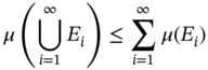
for any disjoint class
 of sets in
  whose union is also in
  . A countably subadditive measure is an outer measure if its domain is the power set of
  , whereby it holds that
  , and
, and  implies
  .
. - 3 Lyapunov exponents are a measure of a system's sensitivity to changes to its initial conditions.
- 4 A contraction map on a metric space
 is a function
  with the property that there is some nonnegative real number
  such that, for all
  ,
,  .
.