
Chapter 6. Queries that Select Records
Query Basics
Creating Queries
Queries and Related Tables
Query Power: Calculated Fields and Text Expressions
Calculated Fields
In a typical database, with thousands or millions of records, you may find it quite a chore finding the information you need. In Chapter 3, you learned how to go on the hunt using the tools of the datasheet, including filtering, searching, and sorting. At first glance, these tools seem like the perfect solution for digging up bits of hard-to-find information. However, there’s a problem: The datasheet features are temporary.
To understand the problem, imagine you’re creating an Access database for a mailorder food company named Boutique Fudge. Using datasheet filtering, sorting, and column hiding, you can pare down the Orders table so it shows only the most expensive orders placed in the past month. (This information’s perfect for targeting big spenders or crafting a hot marketing campaign.) Next, you can apply a different set of settings to find out which customers order more than five pounds of fudge every Sunday. (You could use this information for more detailed market research, or just pass it along to the Department of Health.) But every time you apply new datasheet settings, you lose your previous settings. If you want to jump back from one view to another, then you need to painstakingly reapply all your settings. If you’ve spent some time crafting the perfect view of your data, this process adds up to a lot of unnecessary extra work.
The solution to this problem’s to use queries: ready-made search routines that you store in your database. Even though the Boutique Fudge company has only one Orders table, it may have dozens (or more) queries, each with different sorting and filtering options. If you want to find the most expensive orders, then you don’t need to apply the filtering, sorting, and column hiding settings by hand—instead, you can just fire up the MostExpensiveOrdersLastMonth query, which pulls out just the information you need. Similarly, if you want to find the fudge-a-holics, then you can run the LargeRepeatFudgeOrders query.
Queries are a staple of database design. In this chapter, you’ll learn all you need to design and fine-tune basic queries.
Query Basics
As the name suggests, queries are a way to ask questions about your data, like what products net the most cash, where do most customers live, and who ordered the embroidered toothbrush? Access saves each query in your database, like any other database object (Section 1.1). Once you’ve saved a query, you can run it any time you want to take a look at the live data that meets your criteria.
Queries’ key feature is their amazing ability to reuse your hard work. Queries also introduce some new features that you don’t have with the datasheet alone:
Queries can combine related tables. This feature’s insanely useful because it lets you craft searches that take related data into account. In the Boutique Fudge example, you can use this feature to create queries that find orders with specific product items, or orders made by customers living in specific cities. Both these searches need relationships, because they branch out past the Orders table to take in information from other tables (like Products and Customers). You’ll see how this works in Section 6.3.
Queries can perform calculations. The Products table in the Boutique Fudge database lists price information, along with the quantity in stock. A query can multiply these details, and then add a column that lists the calculated value of the product you have on hand. You’ll try out this trick in Section 6.5.
Queries can automatically apply changes. If you want to find all the orders made by a specific person and reduce the cost of each one by 10 percent, then a query can apply the entire batch of changes in one step. This action requires a different type of query, an action query, which you’ll consider in Chapter 7.
In this chapter, you’ll consider the simplest and most common type of query: the select query, which retrieves a subset of information from a table. Once you’ve retrieved this information, you print or edit it using a datasheet, in the same way you interact with a table.
Creating Queries
Access gives you three ways to create a query:
The Query wizard gives you a quick-and-dirty way to build a simple query. However, this option also gives you the least control.
Design view offers the most common approach to query building. It provides a handy graphical tool that you can use to perfect any query.
SQL view gives you a behind-the-scenes look at the actual query command, which is a piece of text (ranging from one line to more than a dozen) that tells Access exactly what to do. The SQL view’s where many Access experts hang out; for more information on the world of SQL, see Access 2007: The Missing Manual.
Creating a Query in Design View
The best starting point for query creation’s the Design view. The following steps show you how it works. (To try this out yourself, you can use the BoutiqueFudge.accdb database that’s included with the downloadable samples for this chapter.) The final result—a query that gets the results that fall in the first quarter of 2007—is shown in Figure 6-6.
Here’s what you need to do:
Choose Create → Other → Query Design.
A new design window appears, where you can craft your query. But before you get started, Access pops open the Show Table dialog box, where you can choose the tables that you want to work with (Figure 6-1).
Select the table that has the data you want, and then click Add (or just double-click the table).
In the Boutique Fudge example, you need the Orders table.
Access adds a box that represents the table to the design window. You can repeat this step to add several related tables, but for now stick with just one.
Click Close.
The Show Table dialog disappears, giving you access to the Design view for the query.
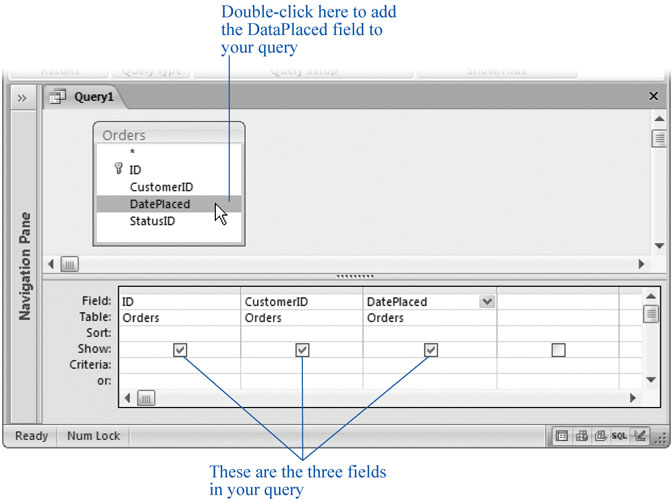
Select the fields you want to include in your query.
To select a field, double-click it in the table box (Figure 6-2). Take care not to add the same field more than once, or that column shows up twice in the results. If you’re using the Boutique Fudge example, then make sure you choose at least the ID, DatePlaced, and CustomerID fields.
Figure 6-1. You’ve seen the Show Table dialog box before—it’s the same way you added tables to the relationships window in Chapter 5.You can double-click the asterisk (*) to choose to include all the columns from a table. However, in most cases, it’s better to add each column separately. Not only does this help you more easily see at a glance what’s in your query, it also lets you choose the column order, and use the field for sorting and filtering.
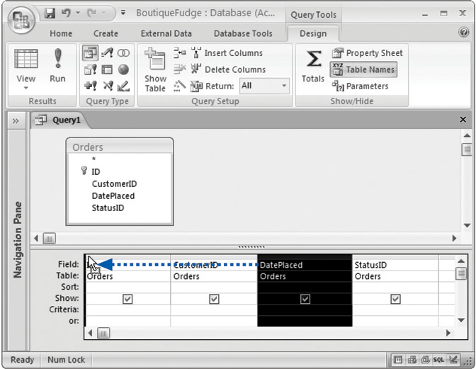
Arrange the fields from left to right in the order you want them to appear in the query results.
When you run the query, the columns appear in the same order as they’re listed in the column list in Design view. (Ordinarily, this system means the columns appear from left to right in the order you added them.) If you want to change the order, then all you need to do is drag (as shown in Figure 6-3).
Figure 6-2. Each time you double-click a field in the table box, Access adds it to the field list at the bottom of the window. You can then configure various settings to control filtering criteria and sorting for that column. If you don’t want to keep mousing back to the table box, then you can add a field directly to the column list by choosing its name from the drop-down Field box.If you want to hide one or more columns, then clear the Show checkbox for those columns.
Ordinarily, Access shows every column you’ve added to the column list. However, in some situations you want to work with a column in your query, but not actually display its data. Usually, it’s because you want to use the column values for sorting or filtering.
Choose a sort order.
If you don’t supply a sort order, then you’ll get the records right from the database in whatever order they happen to be. This convention usually (but not always) means the oldest records appear first, at the top of the table. To sort your table explicitly, choose the field you want to use to sort the results, and then, in the corresponding Sort box, choose a sorting option. In the current example, the table’s sorted by date in descending order, so that the most recent orders are first in the list (Figure 6-4).
Figure 6-3. To reorder your columns, drag the gray bar at the top of the column you want to move to its new home. This technique’s similar to the technique you use to arrange columns in the datasheet (Section 3.1.2). In this example, the DatePlaced field’s being moved to the far left side.Set your filtering criteria.
Filtering (Section 3.2.2) is a tool that lets you focus on the records that interest you and ignore all the rest. Filtering cuts a large swath of data down to the information you need, and it’s the heart of many a query. (You’ll learn much more about building a filter expression in the next section.)
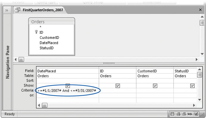
Figure 6-4. Choose Ascending if you want to sort a text field from A-Z, a numeric field from lowest to highest, or a date field from oldest to most recent. Choose Descending to use the reverse order. Section 3.2.1 has more information about sorting and how it applies to different data types.Once you have the filter expression you need, place it into the Criteria box for the appropriate field (Figure 6-5). In the current example, you can put this filter expression in the Criteria box for the DatePlaced field to get the orders placed in the first three months of the year:
>=#1/1/2007# And <=#3/31/2007#
You aren’t limited to a single filter—in fact, you can add a separate filter expression to each field. If you want to use a field for filtering but not display it in the results, then clear the Show checkbox for that field.
Choose Query Tools | Design → Results → Run.
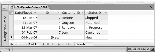
Now that you’ve finished the query, you’re ready to put it into action. When you run the query, you’ll see the results presented in a datasheet (complete with lookups on linked fields), just like when you edit a table. (Figure 6-6 shows the result of the query on the Orders table).
You can switch back to Design view by right-clicking the tab title and then choosing Design View.
Figure 6-5. Here’s a filter that finds orders made in a date range (from January 1 to March 31, in the year 2007). Notice that when you use an actual hard-coded date as part of a condition (like January 1, 2007 in this example), you need to bracket the date with the # symbols. For a refresher about date syntax, refer to Section 4.3.2.2.Figure 6-6. Here are the results of a query that shows orders placed within a specific date range. You can use the datasheet window to review or print your results, or you can edit information just as you would in a table datasheet.Note
The datasheet for your query acquires any formatting you applied to the datasheet of the underlying table. If you applied a hot-pink background and cursive font to the datasheet for the Orders table, then the same settings apply to any queries that use the Orders table. However, you can change the datasheet formatting for your query just as you would with a table.
Save the query.
You can save your query at any time using the keyboard shortcut Ctrl+S. If you don’t, then Access automatically saves your query when you close the query tab (or your entire database). Of course, you don’t need to save your query. Sometimes you might create a query for a specific, one-time-only task. If you don’t plan to reuse the query, then there’s no point in cluttering up your database with extra objects.
The first time you save your query, Access asks for a name. Use the same naming rules that you follow for tables—refrain from using spaces or special characters, and capitalize the first letter in each word. A good query describes the view of data that it presents. One good choice for the example shown in Figure 6-6 is FirstQuarterOrders_2007.


Note
Remember, when you save a query, you aren’t saving the query results—you’re just saving the query design, with all its settings. That way, you can run the query any time to get the live results that match your criteria.
Once you’ve created a query, you’ll see it in your database’s navigation pane (Figure 6-7). If you’re using the standard All Tables view, then the query appears under the table that it uses. If a query uses more than one table, then the same query appears in more than one group in the navigation pane.
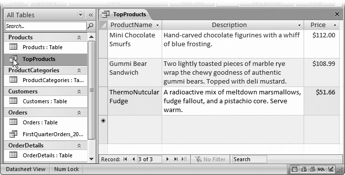
You can launch the query at any time by double-clicking it. Suppose you’ve created a query named TopProducts that grabs all the expensive products in the Products table (using the filter criteria >50 on the Price field). Every time you need to review, print, or edit information about expensive products, you run the TopProducts query. To fine-tune the query settings, right-click it in the navigation pane, and then choose Design View.
Access lets you open your table and any queries that use it at the same time. (They all appear in separate tabs.) However, you can’t modify the design of your table until you close all the queries that use it.
If you add new records to a table while a query’s open, then the new records don’t automatically appear in the query. Instead, you’ll need to run your query again. The quickest way is to choose Home → Records. Refresh → Refresh All. You can also close your query and open it again, because Access runs your query every time you open it in Datasheet view.
Note
Remember, a query’s a view of some of the data in your table. When you edit your query results, Access changes the data in the underlying table. On the other hand, it’s perfectly safe to rename, modify, and delete queries—after all, they’re there to make your life simpler.
Building filter expressions
The secret to a good query’s getting the information you want, and nothing more. To tell Access what records it should get (and which ones it should ignore), you need a filter expression.
The filter expression defines the records you’re interested in. If you want to find all the orders that were placed by a customer with the ID 1032, you could use this filter expression:
=1032
To put this filter expression into action, you need to put it in the Criteria box under the CustomerID field.
Technically, you could just write 1032 instead of =1032, but it’s better to stick to the second form, because that’s the pattern you’ll use for more advanced filter expressions. It starts with the operator (in this case, the equals sign) that defines how Access should compare the information, followed by the value (in this case, 1032) you want to use to make the comparison.
If you’re matching text, then you need to include quotation marks around your value. Otherwise, Access wonders where the text starts and stops:
="Harrington Red"
Instead of using an exact match, you can use a range. Add this filter expression to the OrderTotal field to find all the orders worth between $10 and $50:
<50 And >10
This condition’s actually two conditions (less than 50 and greater than 10), which are yoked together by the powerful And keyword (Section 4.3.2.4). Alternatively, you can use the Or keyword if you want to see results that meet any one of the conditions you’ve included (Section 4.3.2.4).
Date expressions are particularly useful. Just remember to bracket any hardcoded dates with the # character (Section 4.3.2.2). If you add this filter condition to the DatePlaced field, then it finds all the orders that were placed in 2007:
<#1/1/2008# And >#12/31/2006#
This expression works by requiring that dates are earlier than January 1, 2008, but later than December 31, 2006.
Tip
With a little more work, you could craft a filter expression that gets the orders from the first three months of the current year, no matter what year it is. This trick requires the use of the functions Access provides for dates. See Section 4.1.2 for more details.
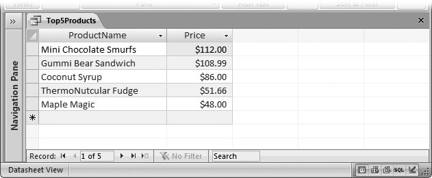
Getting the top records
When you run an ordinary query, you see all the results that match your filter conditions. If that’s more than you bargained for, you can use filter expressions to cut down the list.
However, in some cases, filters are a bit more work than they should be. Imagine a situation where you want to see the top 10 most expensive products. Using a filter condition, you can easily get the products that have prices above a certain threshold. Using sorting, you can arrange the results so the most expensive items turn up at the top. However, you can’t as easily tell Access to get just 10 records and then stop.
In this situation, the query Design view has a shortcut that can help you out. Here’s how it works:
Open your query in Design view (or create a new query and add the fields you want to use).
This example uses the Products table, and includes the ProductName and Price fields.
Sort your table so that the records you’re most interested in are at the top.
If you want to find the most expensive products, then add a descending sort (Section 3.2.1) on the Price field.
In the Query Tools | Design → Query Setup → Return box, choose a different option (Figure 6-8).
The standard option’s All, which gets all the matching records. However, you can choose 5, 25, or 100 to get the top 5, 25, or 100 matching records, respectively. Or, you can use a percentage value like 25 percent to get the top quarter of matching records.
Note
For the Query Tools | Design → Query Setup →Return box to work, you must choose the right sort order. To understand why, you need to know a little more about how this feature works. If you tell Access to get just five records, it actually performs the normal query, gets all the records, and arranges them according to your sort order. It then throws everything away except for the first five records in the list. If you’ve sorted your list so that the most expensive products are first (as in this example), you’re left with the top five budget-busting products in your results.
Run your query to see the results (Figure 6-9).

Creating a Simple Query with the Query Wizard
Design view’s usually the best place to start constructing queries, but it’s not the only option. You can use the Query wizard to give you an initial boost, and then refine your query in Design view.
The Query wizard works by asking you a series of questions, and then creating the query that fits the bill. Unlike many of the other wizards in Access and other Office applications, the Query wizard’s relatively feeble. It’s a good starting point for query newbies, but not an end-to-end performer.
Here’s how you can put the Query wizard to work:
Choose Create → Other → Query Wizard.
Access gives you a choice of several different wizards (Figure 6-10).
Choose a query type. The Simple Query wizard’s the best starting point for now.
The Query wizard includes a few common kinds of queries. With the exception of the crosstab query, there’s nothing really unique about any of these choices. You’ll learn to create them all using Design view:
Simple Query Wizard gets you started with an ordinary query, which displays a subset of data from a table. This query’s the kind you created in the previous section.
Crosstab Query Wizard generates a crosstab query, which lets you summarize large amounts of data using different calculations. You can find more on this advanced topic in Access 2007: The Missing Manual.
Find Duplicates Query Wizard is similar to the Simple Query wizard, except it adds a filter expression that shows only records that share duplicated values. If you forgot to set a primary key or create a unique index for your table (Section 4.1.3), then this can help you clean up the mess.
Find Unmatched Query Wizard is similar to the Simple Query wizard, except it adds a filter expression that finds unlinked records in related tables. You could use this to find an order that isn’t associated with any particular customer. You’ll learn how this works in Section 6.3.2.1.
Click OK.
The first step of the Query wizard appears.
In the Tables/Queries box, choose the table that has the data you want. Then, add the fields you want to see in the query results, as shown in Figure 6-11 .
For the best control, add the fields one at a time. Add them in the order you want them to appear in the query results, from left to right.
You can add fields from more than one table. To do so, start by choosing one of the tables, add the fields you want, and then choose the second table and repeat the process. This process really makes sense only if the tables are related. You’ll learn more in Section 6.3.
Click Next.
If your query includes a numeric field, the Query wizard gives you the choice of creating a summary query that arranges rows into groups, and calculates information like totals and averages. If you get this choice, pick Detail and then click Next.
The final step of the Query wizard appears (Figure 6-12).
Figure 6-11. To add a field, select it in the Available Fields list, and then click the > arrow button (or just double-click it). You can add all fields at once by clicking the >> arrow button, and you can remove fields by selecting them in the Selected Fields list and then clicking <. In this example, three fields are included in the query.Supply a query name in the “What title do you want for your query?” box.
If you want to fine-tune your query, then choose “Modify the query design”. If you’re happy with what you’ve got, then choose “Open the query to view information” to run the query.
One reason you may want to open your query in Design view is to add filter conditions (Section 3.2.2) to pick out specific rows. Unfortunately, you can’t set filter conditions in the Query wizard.
Click Finish.
Your query opens in Design view or Datasheet view, depending on the choice you made in step 7. You can run it by choosing Query Tools | Design → Results → Run.


Queries and Related Tables
In Chapter 5, you learned how to split data down into fundamental pieces and store it in distinct, well-organized tables. This sort of design’s only problem’s that it’s more difficult to get the full picture when you have related data stored in separate places. Fortunately, Access has the perfect solution—you can bring the tables back together for display using a join.
A join’s a query operation that pulls columns from two tables and fuses them together in one grid of results. You use joins to amplify child tables by adding information from the parent table. Here are some examples:
In the bobblehead database, you can show a list of bobblehead dolls (drawn from the child table Dolls) along with the manufacturer information for each doll (from the parent table Manufacturers).
In the Cacophoné music school database, you can get a list of available classes, with instructor information.
In the Boutique Fudge database, you can get a list of orders, complete with the details for the customer who placed the order.
Note
You’ve already learned how to create lookup tables to show just a bit of information from a linked table. A lookup can show the name of a product category in place of the ID number in the ProductID field. However, a join query’s far more powerful. It can grab oodles of information from the linked table—far more than you could fit in a single field.
Figure 6-13 shows how a table join works.
Joining Tables in a Query
Access makes it remarkably easy to join two tables. The first step’s adding both tables to your query, using the Show Table dialog box. If you’re creating a new query in Design view, then the Show Table dialog appears right away. If you’re working with a query you’ve already created, then make sure you’re in Design view, right-click the window, and then choose Show Table.
If you’ve already defined a relationship between the two tables (using the relationships window, as described in Section 5.2), then Access uses that relationship to automatically create a query join. You’ll see a line on the diagram that connects the appropriate fields, as shown in Figure 6-14.

If you haven’t already defined a relationship between the two related tables, then you probably should, before you create your query (see Chapter 5 for full instructions). But if for some cryptic reason you’ve decided not to create the relationship (perhaps the database design was set in stone by another, less savvy Access designer), then you can manually define the join in the query window. To do so, just drag the linked field in one table to the matching field in the other table. You can also remove a join by right-clicking the line between the tables, and then choosing Delete.
Note
If you add two unrelated tables, then Access tries to help you out by guessing a relationship. If it spots a field with the same data type and the same name in both tables, then it adds a join on this field. This action often isn’t what you want—for example, many tables share a common ID field. Also, if you’re following the database design rules from Section 2.5, then your linked fields have slightly different names in each table, like ID and CustomerID. If you run into a problem where Access assumes a relationship that doesn’t exist, then just remove it before adding the join you really want.
Once you have your two tables in the query design window and you’ve defined the join, then you’re ready to choose the fields you want. You can pick fields from both tables. You can also add filter conditions and supply a sort order, as you would with any other query. Figure 6-15 shows an example of a query that uses a join, and Figure 6-16 shows that same query in action.
Note
When you have two linked tables, it’s easy to forget what you’re showing. If you join the Orders and Customers tables, and then select fields from each, then what do you you end up with: a list of classes or a list of instructors? Easy, you get a list of orders, complete with customer information. Queries with linked tables always act on the child table and bring in additional information from the parent.


Note
When you perform a join, you see repeated information. If you join the Customers and Orders tables, you see the first and last name of a shopaholic customer appear next to several orders. However, this doesn’t violate the database rule against duplicate data. Even though the customer details appear in more than one place in the query results, they’re stored only once in the Customers table.
Remember, when you link a parent and child table with a join query, you’re really performing a query that gets all the records from the child table, and then adds extra information from the parent table. For example, you can use a join query to get a list of orders (from the child table) and supplement each record with information about the customer that made the order. No matter how you create the join, you won’t ever get a list of customers with order information tacked on—that wouldn’t make sense, because every customer can make multiple orders.
Joins are one of the most useful features in any query writer’s toolkit. They let you display one table that has all the information you need.
Outer Joins
The queries you saw in the previous example use what database nerds call an inner join. Inner joins show only linked records—in other words, records that appear in both tables. If you perform a query on the Customers and Orders tables, then you don’t see customers that haven’t placed an order. You also don’t see orders that aren’t linked to any particular customer (the CustomerID value’s blank) or aren’t linked to a valid record (they contain a CustomerID value that doesn’t match up to any record in the Customers table).
Outer joins are more accommodating—these joins include all the same results you’d see in an inner join, plus the leftover unlinked records from one of the two tables (it’s your choice). Obviously, these unlinked records show up in the query results with some blank values, which correspond to the missing information that the other table would supply.
Suppose you perform an outer join between the Orders and Customers tables, and then configure it so that all the order records are shown. Any orders that aren’t linked to a customer record appear at the bottom of the list, and have blank values in all the customer-related fields (like FirstName and LastName):
|
FirstName |
LastName |
ID |
DatePlaced |
StatusID |
|
Stanley |
Lem |
7 |
13-Jun-07 |
Cancelled |
|
Toby |
Grayson |
4 |
03-Nov-06 |
Returned |
|
Toby |
Grayson |
6 |
03-Nov-06 |
Shipped |
|
|
|
18 |
01-Jan-08 |
In Progress |
|
19 |
01-Jan-08 |
In Progress |
In this particular example, it doesn’t make sense for orders that aren’t linked to a customer to exist. (In fact, it probably indicates an order that was entered incorrectly.) However, if you suspect a problem, an outer join can help you track down the problem.
Tip
You can prevent orphaned order records altogether by making CustomerID a required value (Section 4.1) and enforcing referential integrity (Section 5.2.3).
You can also perform an outer join between the Orders and Customers tables that shows all the customer records. In this case, at the end of the query results, you’ll see every unlinked customer record, with the corresponding order fields left blank:
|
FirstName |
LastName |
ID |
DatePlaced |
StatusID |
|
Stanley |
Lem7 |
7 |
13-Jun-07 |
Cancelled |
|
Toby |
Grayson |
4 |
03-Nov-06 |
Returned |
|
Toby |
Grayson |
6 |
03-Nov-06 |
Shipped |
|
Ben |
Samatara |
|
|
|
|
Goosey |
Mason |
|
|
|
|
Tabasoum |
Khan |
|
|
|
In this case, the outer join query picks up three stragglers.
So how do you add an outer join to your query? Your start with an inner join (which Access usually adds automatically; see Section 6.3.1), and then convert it to an outer join. To do so, just right-click the join line that links the two tables in the design window, and then choose Join Properties (or just double-click the line). The Join Properties dialog box (Figure 6-17) appears, and lets you change the type of join you’re using.

Finding unmatched records
Inner joins are by far the most common joins. However, outer joins let you create at least one valuable type of query: a query that can track down unmatched records.
You’ve already seen how an outer join lets you see a list of all your orders, plus the customers that haven’t made any orders. That combination isn’t terribly useful. However, the marketing department’s already salivating over the second part of this equation—the list of people who haven’t bought anything. This information could help them target a first-time-buyer promotion.
To craft this query, you start with the outer-join query that includes all the customer records. Then, you simply add one more ingredient: a filter condition that matches records that don’t have an order ID. Technically, these are considered null (empty) values.
Here’s the filter condition you need, which you must place in the Criteria box for the ID field of the Orders table:
Is Null
Now, when Access performs the query, it includes only the customer records that aren’t linked to anything in the orders table. Figure 6-18 shows the query in Design view.

Multiple Joins
Just as you’re getting comfortable with inner and outer joins, Access has another feature to throw your way. Many queries don’t stop at a single join. Instead, they use three, four, or more to bring multiple related tables into the mix.
Although this sounds complicated at first, it really isn’t. Multiple joins are simply ways of bringing more related information into your query. Each join works the same in a multiple-join situation as it does when you use it on its own. To use multiple joins, just add all the tables you want from the Show Table dialog box, make sure the join lines appear, and then choose the fields you want. Access is almost always intelligent enough to figure out what you’re trying to do.
Figure 6-19 shows an example where a child table has two parents that can both contribute some extra information.

Sometimes, the information you want’s more than one table away. Consider the OrderDetails table Boutique Fudge uses to list each item in a customer’s order. On its own, the OrderDetails doesn’t provide a link to the customer who ordered the item, but it does provide a link to the related order record. (See Section 5.4.2.2 for a discussion of this design.) If you want to get the information about who ordered each item, you need to add the OrderDetails, Orders, and Customers table to your query, as shown in Figure 6-20.

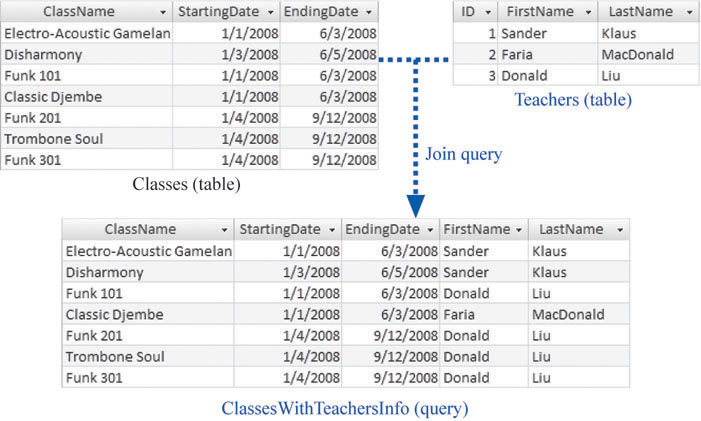
Multiple joins are also the ticket if you have a many-to-many relationship with a junction table (Section 5.3.2), like the one between teachers and classes. As you’ll remember from Chapter 5 (Section 5.4), the Cacophoné Studios music school uses an intermediary table to track teacher class assignment. If you want to get a list of classes, complete with instructor names, then you need to create a query with three tables: Classes, Teachers, and Teachers_Classes (see Figure 6-21).
Query Power: Calculated Fields and Text Expressions
Every Access expert stocks his or her database with a few (or a few dozen) useful queries that simplify day-to-day tasks. Earlier in this chapter, you learned how to create queries that chew through avalanches of information and present exactly what you need to see. But as Access masters know, there’s much more power lurking just beneath the surface of the query design window.

In this section, you’ll delve into some query magic that’s sure to impress your boss, co-workers, and romantic partners. You’ll learn how to carry out calculations in a query and perform some basic text manipulation (joining together first and last names, for example).
Calculated Fields
When you started designing tables, you learned that it’s a database crime to add information that’s based on the data in another field or another table. An example of this mistake is creating a Products table that has both a Price and a PriceWithTax field. The fact that the PriceWithTax field is calculated based on the Price field is a problem. Storing both is a redundant waste of space. Even worse, if the tax rate changes, then you’re left with a lot of records to update and the potential for inconsistent information (like a with-tax price that’s lower than a no-tax price).
Even though you know not to create fields like PriceWithTax, sometimes you will want to see calculated information in Access. Before Boutique Fudge prints a product list for one of its least-loved retailers, it likes to apply a 10 percent price markup. To do this, it needs a way to adjust the price information before printing the data. If the retailer spots the lower price without the markup, they’re sure to demand it.
Queries provide the perfect solution for these kinds of problems, because they include an all-purpose way to mathematically manipulate information. The trick’s to add a calculated field: a field that’s defined in your query, but doesn’t actually exist in the table. Instead, Access calculates the value of a calculated field based on one or more other fields in your table. The values in the calculated field are never stored anywhere—instead, Access generates them each time you run the query.
Defining a Calculated Field
To create a calculated field, you need to supply two details: a name for the field, and an expression that tells Access what calculation it must perform. Calculated fields are defined using this two-part form:
CalculatedFieldName: ExpressionFor example, here’s how you can define the PriceWithTax calculated field:
PriceWithTax: [Price] * 1.10
Essentially, this expression tells Access to take the value from the Price field, and then multiply it by 1.10 (which is equivalent to raising the price by 10 percent). Access repeats this calculation for each record in the query results. For this expression to work, the Price field must exist in the table. However, you don’t need to show the Price field separately in the query results.
You can also refer to the Price field using its full name, which is made up of the table name, followed by a period, followed by the field name, as shown here:
PriceWithTax: [Products].[Price] * 1.10
This syntax is sometimes necessary if your query involves more than one table (using a query join, as described in Section 6.3), and the same field appears in both tables. In this situation, you must use the full name to avoid ambiguity. (If you don’t, Access gives you an error message when you try to run the query.)
To add the PriceWithTax calculated field to a query, you need to use Design view. First, find the column where you want to insert your field. (Usually, you’ll just tack it onto the end in the first blank column, although you can drag the other fields around to make space.) Next, type the full definition for the field into the Field box (see Figure 6-22).

Now you’re ready to run the query. When you do, the calculated information appears alongside your other columns (Figure 6-23).
Calculated fields do have one limitation—since the information isn’t stored in your table, you can’t edit it. If you want to make a price change, you’ll need to edit the underlying Price field—trying to change PriceWithTax would leave Access thoroughly confused.

Before going any further, it’s worth reviewing the rules of calculated fields. Here are some pointers:
Always choose a unique name. An expression like Price: [Price] * 1.10 creates a circular reference, because the name of the field you’re using is the same as the name of the field you’re trying to create. Access doesn’t allow this sleight of hand.
Build expressions out of fields, numbers, and math operations. The most common calculated fields take one or more existing fields or hard-coded numbers and combine them using familiar math symbols like addition (+), subtraction (-), multiplication (*), or division (/).
Expect to see square brackets. The expression PriceWithTax: [Price] * 1.10 is equivalent to PriceWithTax: Price * 1.10 (the only difference is the square brackets around the field name Price). Technically, you need the brackets only if your field name contains spaces or special characters. However, when you type in expressions that don’t use brackets in the query Design view, then Access automatically adds them, just to be on the safe side.
Simple Math with Numeric Fields
Many calculated fields rely entirely on ordinary high school math. Table 6-1 gives a quick overview of your basic options for combining numbers.
You’re free to use as many fields and operators as you need to create your expression. Consider a Products table with a QuantityInStock field that records the number of units in your warehouse. To determine the value you have on hand for a given product, you can write this expression that uses two fields:
ValueInStock: [UnitsInStock] * [Price]
Warning
When performing a mathematical operation with a field, you’ll run into trouble if the field contains a blank value.
Date fields
You can also use the addition and subtraction operators with date fields. (You can use multiplication, division, and everything else, but it doesn’t have any realistic meaning.)
Using addition, you can add an ordinary number to a date field. This number moves the date forward by that many days. Here’s an example that adds two weeks of headroom to a company deadline:
ExtendedDeadline: [DueDate] + 14
If you use this calculation with the date January 10, 2007, the new date becomes January 24, 2007.
Using subtraction, you can find the number of days between any two dates. Here’s how you calculate how long it was between the time an order was placed and when it was shipped:
ShippingLag: [ShipDate] - [OrderDate]
If the ship date occurred 12 days after the order date, you’d see a value of 12.
Note
Date fields can include time information. In calculations, the time information’s represented as the fractional part of the value. If you subtract two dates and wind up with the number 12.25, that represents 12 days and six hours (because six hours is 25 percent of a full day).
Remember, if you want to include literal dates in your queries (specific dates you supply), you need to bracket them with the # character and use Month/Day/Year format. Here’s an example that uses that approach to count the number of days between the date students were expected to submit an assignment (March 20, 2007) and the date they actually did:
LateDays: [DateSubmitted] - #03/20/07#
A positive value indicates that the value in DateSubmitted is larger (more recent) than the deadline date—in other words, the student was late. A value of 4 indicates a student that’s four days off the mark, while–4 indicates a student that handed the work in four days ahead of schedule.
Order of operations
If you have a long string of calculations, Access follows the standard rules for order of operations: mathematician-speak for deciding which calculation to perform first when there’s more than one calculation in an expression. So if you have a lengthy expression, Access doesn’t just carry on from left to right. Instead, it evaluates the expression piece by piece in this order:
Suppose you want to take the QuantityInStock and the QuantityOnOrder fields into consideration to determine the value of all the product you have available and on the way. If you’re not aware of the order of operation rules, then you might try this expression:
TotalValue: [UnitsInStock] + [UnitsOnOrder] * [Price]
The problem here is that Access multiplies QuantityOnOrder and Price together, and then adds it to the QuantityInStock. To correct this oversight, you need parentheses like so:
TotalValue: ([UnitsInStock] + [UnitsOnOrder]) * [Price]
Now the QuantityInStock and QuantityOnOrder fields are totaled together, and then multiplied with the Price to get a grand total.
Tip
Need some more space to write a really long expression? You can widen any column in the query designer to see more at once, but you’ll still have trouble with complex calculations. Better to click in the Field box, and then press Shift+F2. This action pops open a dialog box named Zoom, which shows the full content in a large text box, wrapped over as many lines as necessary. When you’ve finished reviewing or editing your expression, click OK to close the Zoom box and keep any changes you’ve made, or Cancel to discard them.
Expressions with Text
Although calculated fields usually deal with numeric information, they don’t always. You have genuinely useful ways to manipulate text as well.
If you have text information, then you obviously can’t use addition, subtraction, and other mathematical operations. However, you can join text together. You can, for instance, link several fields of address information together and show them all in one field, conserving space (and possibly making it easier to export the information to another program).
To join text, you use the ampersand (&) operator. For example, here’s how to create a FullName field that draws information from the FirstName and LastName fields:
FullName: [FirstName] & [LastName]
This expression looks reasonable enough, but it’s actually got a flaw. Since you haven’t added any spaces, the first and last name end up crammed together, like this: BenJenks. A better approach is to join together three pieces of text: the first name, a space, and the last name. Here’s the revised expression:
FullName: [FirstName] & " " & [LastName]
This produces values like Ben Jenks. You can also swap the order and add a comma, if you prefer to have the last name first (like Jenks, Ben) for better sorting:
FullName: [LastName] & ", " & [FirstName]
Note
Access has two types of text values: those you draw from other fields, and those you enter directly (or hard-code). When you hard-code a piece of text (such as the comma and space in the previous example), you need to wrap it in quotation marks so Access knows where it starts and stops.
You can even use the ampersand to tack text alongside numeric values. If you want the slightly useless text “The price is” to appear before each price value, use this calculated field:
Price: "The price is: " & [Price]