Terminology

This chapter makes use of a set of terms specific to the finance domain. We’ll briefly define them here:

Instrument

A tradable asset, such as a bond, loan, option, or stock investment. At any particular time, an instrument is considered to have a value, which is the price for which it could be sold.

Portfolio

A collection of instruments owned by a financial institution.

Return

The change in an instrument or portfolio’s value over a time period.

Loss

A negative return.

Index

An imaginary portfolio of instruments. For example, the NASDAQ Composite Index includes about 3,000 stocks and similar instruments for major US and international companies.

Market factor

A value that can be used as an indicator of macroaspects of the financial climate at a particular time—for example, the value of an index, the gross domestic product of the United States, or the exchange rate between the dollar and the euro. We will often refer to market factors as just factors.

Methods for Calculating VaR

So far, our definition of VaR has been fairly open-ended. Estimating this statistic requires proposing a model for how a portfolio functions and choosing the probability distribution its returns are likely to take. Institutions employ a variety of approaches for calculating VaR, all of which tend to fall under a few general methods.

Our Model

A Monte Carlo risk model typically phrases each instrument’s return in terms of a set of market factors. Common market factors might be the value of indexes like the S&P 500, the US GDP, or currency exchange rates. We then need a model that predicts the return of each instrument based on these market conditions. In our simulation, we’ll use a simple linear model. By our previous definition of return, a factor return is a change in the value of a market factor over a particular time. For example, if the value of the S&P 500 moves from 2,000 to 2,100 over a time interval, its return would be 100. We’ll derive a set of features from simple transformations of the factor returns. That is, the market factor vector m_t for a trial t is transformed by some function φ to produce a feature vector of possible different length f_t:

• f_t = ϕ(m_t)

For each instrument, we’ll train a model that assigns a weight to each feature. To calculate r_it, the return of instrument i in trial t, we use c_i, the intercept term for the instrument; w_ij, the regression weight for feature j on instrument i; and f_tj, the randomly generated value of feature j in trial t:

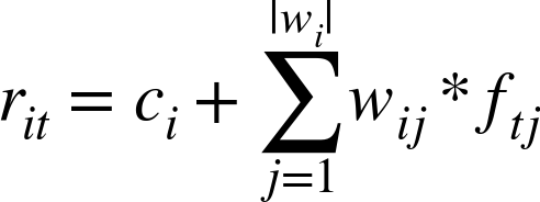
This means that the return of each instrument is calculated as the sum of the returns of the market factor features multiplied by their weights for that instrument. We can fit the linear model for each instrument using historical data (also known as doing linear regression). If the horizon of the VaR calculation is two weeks, the regression treats every (overlapping) two-week interval in history as a labeled point.

It’s also worth mentioning that we could have chosen a more complicated model. For example, the model need not be linear: it could be a regression tree or explicitly incorporate domain-specific knowledge.

Now that we have our model for calculating instrument losses from market factors, we need a process for simulating the behavior of market factors. A simple assumption is that each market factor return follows a normal distribution. To capture the fact that market factors are often correlated—when NASDAQ is down, the Dow is likely to be suffering as well—we can use a multivariate normal distribution with a non-diagonal covariance matrix:

where μ is a vector of the empirical means of the returns of the factors and Σ is the empirical covariance matrix of the returns of the factors.

As before, we could have chosen a more complicated method of simulating the market or assumed a different type of distribution for each market factor, perhaps using distributions with fatter tails.

Getting the Data

It can be difficult to find large volumes of nicely formatted historical price data, but Yahoo! has a variety of stock data available for download in CSV format. The following script, located in the risk/data directory of the repo, will make a series of REST calls to download histories for all the stocks included in the NASDAQ index and place them in a stocks/ directory:

$ ./download-all-symbols.sh

We also need historical data for risk factors. For our factors, we’ll use the values of the S&P 500 and NASDAQ indexes, as well as the prices of 5-year and 30-year US Treasury bonds. These can all be downloaded from Yahoo! as well:

$ mkdir factors/
$ ./download-symbol.sh ^GSPC factors
$ ./download-symbol.sh ^IXIC factors
$ ./download-symbol.sh ^TYX factors
$ ./download-symbol.sh ^FVX factors

Preprocessing

The first few rows of the Yahoo!-formatted data for GOOGL looks like:

Date,Open,High,Low,Close,Volume,Adj Close
2014-10-24,554.98,555.00,545.16,548.90,2175400,548.90
2014-10-23,548.28,557.40,545.50,553.65,2151300,553.65
2014-10-22,541.05,550.76,540.23,542.69,2973700,542.69
2014-10-21,537.27,538.77,530.20,538.03,2459500,538.03
2014-10-20,520.45,533.16,519.14,532.38,2748200,532.38

Let’s fire up the PySpark shell. In this chapter, we rely on several libraries to make our lives easier. The GitHub repo contains a Maven project that can be used to build a JAR file that packages all these dependencies together:

$ cd ch09-risk/
$ mvn package
$ cd data/
$ pyspark-shell --jars ../target/ch09-risk-2.0.0-jar-with-dependencies.jar

For each instrument and factor, we want to derive a list of (date, closing price) tuples. The java.time library contains useful functionality for representing and manipulating dates. We can represent our dates as LocalDate objects. We can use the DateTimeFormatter to parse dates in the Yahoo date format:

import java.time.LocalDate
import java.time.format.DateTimeFormatter

val format = DateTimeFormatter.ofPattern("yyyy-MM-dd")
LocalDate.parse("2014-10-24")
res0: java.time.LocalDate = 2014-10-24

The 3,000-instrument histories and 4-factor histories are small enough to read and process locally. This remains the case even for larger simulations with hundreds of thousands of instruments and thousands of factors. The need arises for a distributed system like PySpark when we’re actually running the simulations, which can require massive amounts of computation on each instrument.

To read a full Yahoo history from local disk:

import java.io.File

def readYahooHistory(file: File): Array[(LocalDate, Double)] = {
  val formatter = DateTimeFormatter.ofPattern("yyyy-MM-dd")
  val lines = python.io.Source.fromFile(file).getLines().toSeq
  lines.tail.map { line =>
    val cols = line.split(',')
    val date = LocalDate.parse(cols(0), formatter)
    val value = cols(1).toDouble
    (date, value)
  }.reverse.toArray
}

Notice that lines.tail is useful for excluding the header row. We load all the data and filter out instruments with less than five years of history:

val start = LocalDate.of(2009, 10, 23)
val end = LocalDate.of(2014, 10, 23)

val stocksDir = new File("stocks/")
val files = stocksDir.listFiles()
val allStocks = files.iterator.flatMap { file =>> 
  try {
    Some(readYahooHistory(file))
  } catch {
    case e: Exception => None
  }
}
val rawStocks = allStocks.filter(_.size >= 260 * 5 + 10)

val factorsPrefix = "factors/"
val rawFactors = Array(
  "^GSPC.csv", "^IXIC.csv", "^TYX.csv", "^FVX.csv").
  map(x => new File(factorsPrefix + x)).
  map(readYahooHistory)

Using iterator here allows us to stream over the files instead of loading their full contents in memory all at once.

Different types of instruments may trade on different days, or the data may have missing values for other reasons, so it is important to make sure that our different histories align. First, we need to trim all of our time series to the same region in time. Then we need to fill in missing values. To deal with time series that are missing values at the start and end dates in the time region, we simply fill in those dates with nearby values in the time region:

def trimToRegion(history: Array[(LocalDate, Double)],
    start: LocalDate, end: LocalDate)
  : Array[(LocalDate, Double)] = {
  var trimmed = history.dropWhile(_._1.isBefore(start)).
    takeWhile(x => x._1.isBefore(end) || x._1.isEqual(end))
  if (trimmed.head._1 != start) {
    trimmed = Array((start, trimmed.head._2)) ++ trimmed
  }
  if (trimmed.last._1 != end) {
    trimmed = trimmed ++ Array((end, trimmed.last._2))
  }
  trimmed
}

To deal with missing values within a time series, we use a simple imputation strategy that fills in an instrument’s price as its most recent closing price before that day. Because there is no pretty python Collections method that can do this for us, we write it on our own. The spark-ts and flint libraries are alternatives that contain an array of useful time series manipulations functions.

import python.collection.mutable.ArrayBuffer

def fillInHistory(history: Array[(DateTime, Double)],
    start: DateTime, end: DateTime): Array[(DateTime, Double)] = {
  var cur = history
  val filled = new ArrayBuffer[(DateTime, Double)]()
  var curDate = start
  while (curDate < end) {
    if (cur.tail.nonEmpty && cur.tail.head._1 == curDate) {
      cur = cur.tail
    }

    filled += ((curDate, cur.head._2))

    curDate += 1.days
    // Skip weekends
    if (curDate.dayOfWeek().get > 5) curDate += 2.days
  }
  filled.toArray
}

We apply trimToRegion and fillInHistory to the data:

val stocks = rawStocks.
  map(trimToRegion(_, start, end)).
  map(fillInHistory(_, start, end))

val factors = (factors1 ++ factors2).
  map(trimToRegion(_, start, end)).
  map(fillInHistory(_, start, end))

Keep in mind that, even though the python APIs used here look very similar to PySpark’s API, these operations are executing locally. Each element of stocks is an array of values at different time points for a particular stock. factors has the same structure. All these arrays should have equal length, which we can verify with:

(stocks ++ factors).forall(_.size == stocks(0).size)
res17: Boolean = true

Determining the Factor Weights

Recall that VaR deals with losses over a particular time horizon. We are not concerned with the absolute prices of instruments but how those prices move over a given length of time. In our calculation, we will set that length to two weeks. The following function makes use of the python Collections’ sliding method to transform time series of prices into an overlapping sequence of price movements over two-week intervals. Note that we use 10 instead of 14 to define the window because financial data does not include weekends:

def twoWeekReturns(history: Array[(LocalDate, Double)])
  : Array[Double] = {
  history.sliding(10).
    map { window =>
      val next = window.last._2
      val prev = window.head._2
      (next - prev) / prev
    }.toArray
}

val stocksReturns = stocks.map(twoWeekReturns).toArray.toSeq 
val factorsReturns = factors.map(twoWeekReturns)

Because of our earlier use of iterator, stocks is an iterator. .toArray.toSeq runs through it and collects the elements in memory into a sequence.

With these return histories in hand, we can turn to our goal of training predictive models for the instrument returns. For each instrument, we want a model that predicts its two-week return based on the returns of the factors over the same time period. For simplicity, we will use a linear regression model.

To model the fact that instrument returns may be nonlinear functions of the factor returns, we can include some additional features in our model that we derive from nonlinear transformations of the factor returns. We will try adding two additional features for each factor return: square and square root. Our model is still a linear model in the sense that the response variable is a linear function of the features. Some of the features just happen to be determined by nonlinear functions of the factor returns. Keep in mind that this particular feature transformation is meant to demonstrate some of the options available—it shouldn’t be perceived as a state-of-the-art practice in predictive financial modeling.

Even though we will be carrying out many regressions—one for each instrument—the number of features and data points in each regression is small, meaning that we don’t need to make use of PySpark’s distributed linear modeling capabilities. Instead, we’ll use the ordinary least squares regression offered by the Apache Commons Math package. While our factor data is currently a Seq of histories (each an array of (DateTime, Double) tuples), OLSMultipleLinearRegression expects data as an array of sample points (in our case a two-week interval), so we need to transpose our factor matrix:

def factorMatrix(histories: Seq[Array[Double]])
  : Array[Array[Double]] = {
  val mat = new Array[Array[Double]](histories.head.length)
  for (i <- histories.head.indices) {
    mat(i) = histories.map(_(i)).toArray
  }
  mat
}

val factorMat = factorMatrix(factorsReturns)

Then we can tack on our additional features:

def featurize(factorReturns: Array[Double]): Array[Double] = {
  val squaredReturns = factorReturns.
    map(x => math.signum(x) * x * x)
  val squareRootedReturns = factorReturns.
    map(x => math.signum(x) * math.sqrt(math.abs(x)))
  squaredReturns ++ squareRootedReturns ++ factorReturns
}

val factorFeatures = factorMat.map(featurize)

And then we can fit the linear models. In addition, to find the model parameters for each instrument, we can use the OLSMultipleLinearRegression’s estimateRegressionParameters method:

import org.apache.commons.math3.stat.regression.OLSMultipleLinearRegression

def linearModel(instrument: Array[Double],
    factorMatrix: Array[Array[Double]])
  : OLSMultipleLinearRegression = {
  val regression = new OLSMultipleLinearRegression()
  regression.newSampleData(instrument, factorMatrix)
  regression
}

val factorWeights = stocksReturns.
  map(linearModel(_, factorFeatures)).
  map(_.estimateRegressionParameters()).
  toArray

We now have a 1,867×8 matrix where each row is the set of model parameters (coefficients, weights, covariants, regressors, or whatever you wish to call them) for an instrument.

We will elide this analysis for brevity, but at this point in any real-world pipeline it would be useful to understand how well these models fit the data. Because the data points are drawn from time series, and especially because the time intervals are overlapping, it is very likely that the samples are autocorrelated. This means that common measures like R² are likely to overestimate how well the models fit the data. The Breusch-Godfrey test is a standard test for assessing these effects. One quick way to evaluate a model is to separate a time series into two sets, leaving out enough data points in the middle so that the last points in the earlier set are not autocorrelated with the first points in the later set. Then train the model on one set and look at its error on the other.

Sampling

With our models that map factor returns to instrument returns in hand, we now need a procedure for simulating market conditions by generating random factor returns. That is, we need to decide on a probability distribution over factor return vectors and sample from it. What distribution does the data actually take? It can often be useful to start answering this kind of question visually. A nice way to visualize a probability distribution over continuous data is a density plot that plots the distribution’s domain versus its PDF. Because we don’t know the distribution that governs the data, we don’t have an equation that can give us its density at an arbitrary point, but we can approximate it through a technique called kernel density estimation. In a loose way, kernel density estimation is a way of smoothing out a histogram. It centers a probability distribution (usually a normal distribution) at each data point. So a set of two-week-return samples would result in 200 normal distributions, each with a different mean. To estimate the probability density at a given point, it evaluates the PDFs of all the normal distributions at that point and takes their average. The smoothness of a kernel density plot depends on its bandwidth, the standard deviation of each of the normal distributions. The GitHub repository comes with a kernel density implementation that works both over RDDs and local collections. For brevity, it is elided here.

breeze-viz is a python library that makes it easy to draw simple plots. The following snippet creates a density plot from a set of samples:

import org.apache.pyspark.mllib.stat.KernelDensity
import org.apache.pyspark.util.StatCounter
import breeze.plot._

def plotDistribution(samples: Array[Double]): Figure = {
  val min = samples.min
  val max = samples.max
  val stddev = new StatCounter(samples).stdev
  val bandwidth = 1.06 * stddev * math.pow(samples.size, -0.2) 

  val domain = Range.Double(min, max, (max - min) / 100).
    toList.toArray
  val kd = new KernelDensity().
    setSample(samples.toSeq.toDS.rdd).
    setBandwidth(bandwidth)
  val densities = kd.estimate(domain)
  val f = Figure()
  val p = f.subplot(0)
  p += plot(domain, densities)
  p.xlabel = "Two Week Return ($)"
  p.ylabel = "Density"
  f
}

plotDistribution(factorsReturns(0))
plotDistribution(factorsReturns(2))

We use what is known as “Silverman’s rule of thumb,” named after the British statistician Bernard Silverman, to pick a reasonable bandwidth.

Figure 6-1 shows the distribution (probability density function) of two-week returns for the S&P 500 in our history.

Figure 6-1. Two-week S&P 500 returns distribution

Figure 6-2 shows the same for two-week returns of 30-year Treasury bonds.

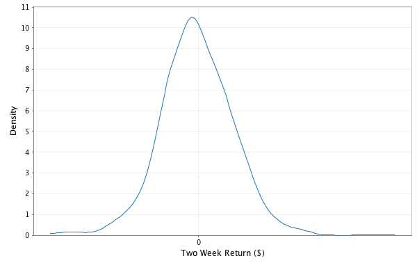
Figure 6-2. Two-week 30-year Treasury bond returns distribution

We will fit a normal distribution to the returns of each factor. Looking for a more exotic distribution, perhaps with fatter tails, that more closely fits the data is often worthwhile. However, for the sake of simplicity, we will avoid tuning our simulation in this way.

The simplest way to sample factors’ returns would be to fit a normal distribution to each of the factors and sample from these distributions independently. However, this ignores the fact that market factors are often correlated. If the S&P is down, the Dow is likely to be down as well. Failing to take these correlations into account can give us a much rosier picture of our risk profile than its reality. Are the returns of our factors correlated? The Pearson’s correlation implementation from Commons Math can help us find out:

import org.apache.commons.math3.stat.correlation.PearsonsCorrelation

val factorCor =
  new PearsonsCorrelation(factorMat).getCorrelationMatrix().getData()
println(factorCor.map(_.mkString("	")).mkString("
"))
1.0       -0.3472   0.4424    0.4633 
-0.3472   1.0       -0.4777   -0.5096
0.4424    -0.4777   1.0       0.9199
0.4633    -0.5096   0.9199    1.0

Digits truncated to fit within the margins

Because we have nonzero elements off the diagonals, it doesn’t look like it.

import org.apache.commons.math3.stat.correlation.Covariance

val factorCov = new Covariance(factorMat).getCovarianceMatrix().
  getData()

val factorMeans = factorsReturns.
  map(factor => factor.sum / factor.size).toArray

import org.apache.commons.math3.distribution.MultivariateNormalDistribution

val factorsDist = new MultivariateNormalDistribution(factorMeans,
  factorCov)

factorsDist.sample()
res1: Array[Double] = Array(-0.05782773255967754, 0.01890770078427768,
  0.029344325473062878, 0.04398266164298203)

factorsDist.sample()
res2: Array[Double] = Array(-0.009840154244155741, -0.01573733572551166,
  0.029140934507992572, 0.028227818241305904)

Running the Trials

With the per-instrument models and a procedure for sampling factor returns, we now have the pieces we need to run the actual trials. Because running the trials is very computationally intensive, we will finally turn to PySpark to help us parallelize them. In each trial, we want to sample a set of risk factors, use them to predict the return of each instrument, and sum all those returns to find the full trial loss. To achieve a representative distribution, we want to run thousands or millions of these trials.

We have a few choices for how to parallelize the simulation. We can parallelize along trials, instruments, or both. To parallelize along both, we would create a data set of instruments and a data set of trial parameters, and then use the crossJoin transformation to generate a data set of all the pairs. This is the most general approach, but it has a couple of disadvantages. First, it requires explicitly creating an RDD of trial parameters, which we can avoid by using some tricks with random seeds. Second, it requires a shuffle operation.

Partitioning along instruments would look something like this:

val randomSeed = 1496
val instrumentsDS = ...
def trialLossesForInstrument(seed: Long, instrument: Array[Double])
  : Array[(Int, Double)] = {
  ...
}
instrumentsDS.flatMap(trialLossesForInstrument(randomSeed, _)).
  reduceByKey(_ + _)

With this approach, the data is partitioned across an RDD of instruments, and for each instrument a flatMap transformation computes and yields the loss against every trial. Using the same random seed across all tasks means that we will generate the same sequence of trials. A reduceByKey sums together all the losses corresponding to the same trials. A disadvantage of this approach is that it still requires shuffling O(|instruments| * |trials|) data.

Our model data for our few thousand instruments data is small enough to fit in memory on every executor, and some back-of-the-envelope calculations reveal that this is probably still the case even with a million or so instruments and hundreds of factors. A million instruments times 500 factors times the 8 bytes needed for the double that stores each factor weight equals roughly 4 GB, small enough to fit in each executor on most modern-day cluster machines. This means that a good option is to distribute the instrument data in a broadcast variable. The advantage of each executor having a full copy of the instrument data is that total loss for each trial can be computed on a single machine. No aggregation is necessary.

With the partition-by-trials approach (which we will use), we start out with an RDD of seeds. We want a different seed in each partition so that each partition generates different trials:

val parallelism = 1000
val baseSeed = 1496

val seeds = (baseSeed until baseSeed + parallelism)
val seedDS = seeds.toDS().repartition(parallelism)

Random number generation is a time-consuming and CPU-intensive process. While we don’t employ this trick here, it can often be useful to generate a set of random numbers in advance and use it across multiple jobs. The same random numbers should not be used within a single job, because this would violate the Monte Carlo assumption that the random values are independently distributed. If we were to go this route, we would replace toDS with textFile and load randomNumbersDS.

For each seed, we want to generate a set of trial parameters and observe the effects of these parameters on all the instruments. Let’s start from the ground up by writing a function that calculates the return of a single instrument underneath a single trial. We simply apply the linear model that we trained earlier for that instrument. The length of the instrument array of regression parameters is one greater than the length of the trial array, because the first element of the instrument array contains the intercept term:

def instrumentTrialReturn(instrument: Array[Double],
    trial: Array[Double]): Double = {
  var instrumentTrialReturn = instrument(0)
  var i = 0
  while (i < trial.length) { 
    instrumentTrialReturn += trial(i) * instrument(i+1)
    i += 1
  }
  instrumentTrialReturn
}

We use a while loop here instead of a more functional python construct because this is a performance-critical region.

Then, to calculate the full return for a single trial, we simply average over the returns of all the instruments. This assumes that we’re holding an equal value of each instrument in the portfolio. A weighted average would be used if we held different amounts of each stock.

def trialReturn(trial: Array[Double],
    instruments: Seq[Array[Double]]): Double = {
  var totalReturn = 0.0
  for (instrument <- instruments) {
    totalReturn += instrumentTrialReturn(instrument, trial)
  }
  totalReturn / instruments.size
}

Lastly, we need to generate a bunch of trials in each task. Because choosing random numbers is a big part of the process, it is important to use a strong random number generator that will take a very long time to repeat itself. Commons Math includes a Mersenne Twister implementation that is good for this. We use it to sample from a multivariate normal distribution as described previously. Note that we are applying the featurize method that we defined before on the generated factor returns in order to transform them into the feature representation used in our models:

import org.apache.commons.math3.random.MersenneTwister

def trialReturns(seed: Long, numTrials: Int,
    instruments: Seq[Array[Double]], factorMeans: Array[Double],
    factorCovariances: Array[Array[Double]]): Seq[Double] = {
  val rand = new MersenneTwister(seed)
  val multivariateNormal = new MultivariateNormalDistribution(
    rand, factorMeans, factorCovariances)

  val trialReturns = new Array[Double](numTrials)
  for (i <- 0 until numTrials) {
    val trialFactorReturns = multivariateNormal.sample()
    val trialFeatures = featurize(trialFactorReturns)
    trialReturns(i) = trialReturn(trialFeatures, instruments)
  }
  trialReturns
}

With our scaffolding complete, we can use it to compute an RDD where each element is the total return from a single trial. Because the instrument data (matrix including a weight on each factor feature for each instrument) is large, we use a broadcast variable for it. This ensures that it only needs to be deserialized once per executor:

val numTrials = 10000000

val trials = seedDS.flatMap(
  trialReturns(_, numTrials / parallelism,
    factorWeights, factorMeans, factorCov))

trials.cache()

If you recall, the whole reason we’ve been messing around with all these numbers is to calculate VaR. trials now forms an empirical distribution over portfolio returns. To calculate 5% VaR, we need to find a return that we expect to underperform 5% of the time, and a return that we expect to outperform 5% of the time. With our empirical distribution, this is as simple as finding the value that 5% of trials are worse than and 95% of trials are better than. We can accomplish this using the takeOrdered action to pull the worst 5% of trials into the driver. Our VaR is the return of the best trial in this subset:

def fivePercentVaR(trials: Dataset[Double]): Double = {
  val quantiles = trials.stat.approxQuantile("value",
    Array(0.05), 0.0)
  quantiles.head
}

val valueAtRisk = fivePercentVaR(trials)
valueAtRisk: Double = -0.010831826593164014

We can find the CVaR with a nearly identical approach. Instead of taking the best trial return from the worst 5% of trials, we take the average return from that set of trials:

def fivePercentCVaR(trials: Dataset[Double]): Double = {
  val topLosses = trials.orderBy("value").
    limit(math.max(trials.count().toInt / 20, 1))
  topLosses.agg("value" -> "avg").first()(0).asInstanceOf[Double]
}

val conditionalValueAtRisk = fivePercentCVaR(trials)
conditionalValueAtRisk: Double = -0.09002629251426077

Visualizing the Distribution of Returns

In addition to calculating VaR at a particular confidence level, it can be useful to look at a fuller picture of the distribution of returns. Are they normally distributed? Do they spike at the extremities? As we did for the individual factors, we can plot an estimate of the probability density function for the joint probability distribution using kernel density estimation (see Figure 6-3). Again, the supporting code for calculating the density estimates in a distributed fashion (over RDDs) is included in the GitHub repository accompanying this book:

import org.apache.spark.sql.functions

def plotDistribution(samples: Dataset[Double]): Figure = {
  val (min, max, count, stddev) = samples.agg(
    functions.min($"value"),
    functions.max($"value"),
    functions.count($"value"),
    functions.stddev_pop($"value")
  ).as[(Double, Double, Long, Double)].first()
  val bandwidth = 1.06 * stddev * math.pow(count, -0.2) 

  // Using toList before toArray avoids a python bug
  val domain = Range.Double(min, max, (max - min) / 100).
    toList.toArray
  val kd = new KernelDensity().
    setSample(samples.rdd).
    setBandwidth(bandwidth)
  val densities = kd.estimate(domain)
  val f = Figure()
  val p = f.subplot(0)
  p += plot(domain, densities)
  p.xlabel = "Two Week Return ($)"
  p.ylabel = "Density"
  f
}

plotDistribution(trials)

Again, Silverman’s rule of thumb.

Figure 6-3. Two-week returns distribution

Evaluating Our Results

How do we know whether our estimate is a good estimate? How do we know whether we should simulate with a larger number of trials? In general, the error in a Monte Carlo simulation should be proportional to . This means that, in general, quadrupling the number of trials should approximately cut the error in half.

A nice way to get a confidence interval on our VaR statistic is through bootstrapping. We achieve a bootstrap distribution over the VaR by repeatedly sampling with replacement from the set of portfolio return results of our trials. Each time, we take a number of samples equal to the full size of the trials set and compute a VaR from those samples. The set of VaRs computed from all the times form an empirical distribution, and we can get our confidence interval by simply looking at its quantiles.

The following is a function that will compute a bootstrapped confidence interval for any statistic (given by the computeStatistic argument) of an RDD. Notice its use of PySpark’s sample where we pass true for its first argument withReplacement, and 1.0 for its second argument to collect a number of samples equal to the full size of the data set:

def bootstrappedConfidenceInterval(
    trials: Dataset[Double],
    computeStatistic: Dataset[Double] => Double,
    numResamples: Int,
    probability: Double): (Double, Double) = {
  val stats = (0 until numResamples).map { i =>
    val resample = trials.sample(true, 1.0)
    computeStatistic(resample)
  }.sorted
  val lowerIndex = (numResamples * probability / 2 - 1).toInt
  val upperIndex = math.ceil(numResamples * (1 - probability / 2))
    .toInt
  (stats(lowerIndex), stats(upperIndex))
}

Then we call this function, passing in the fivePercentVaR function we defined earlier that computes the VaR from an RDD of trials:

bootstrappedConfidenceInterval(trials, fivePercentVaR, 100, .05)
...
(-0.019480970253736192,-1.4971191125093586E-4)

We can bootstrap the CVaR as well:

bootstrappedConfidenceInterval(trials, fivePercentCVaR, 100, .05)
...
(-0.10051267317397554,-0.08058996149775266)

The confidence interval helps us understand how confident our model is in its result, but it does little to help us understand how well our model matches reality. Backtesting on historical data is a good way to check the quality of a result. One common test for VaR is Kupiec’s proportion-of-failures (POF) test. It considers how the portfolio performed at many historical time intervals and counts the number of times the losses exceeded the VaR. The null hypothesis is that the VaR is reasonable, and a sufficiently extreme test statistic means that the VaR estimate does not accurately describe the data. The test statistic—which relies on p, the confidence level parameter of the VaR calculation; x, the number of historical intervals over which the losses exceeded the VaR; and T, the total number of historical intervals considered—is computed as:

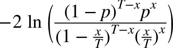
The following computes the test statistic on our historical data. We expand out the logs for better numerical stability:

var failures = 0
for (i <- stocksReturns.head.indices) {
  val loss = stocksReturns.map(_(i)).sum / stocksReturns.size
  if (loss < valueAtRisk) {
    failures += 1
  }
}
failures
...
257

val total = stocksReturns.size
val confidenceLevel = 0.05
val failureRatio = failures.toDouble / total
val logNumer = ((total - failures) * math.log1p(-confidenceLevel) +
  failures * math.log(confidenceLevel))
val logDenom = ((total - failures) * math.log1p(-failureRatio) +
  failures * math.log(failureRatio))
val testStatistic = -2 * (logNumer - logDenom)
...
180.3543986286574

If we assume the null hypothesis that the VaR is reasonable, then this test statistic is drawn from a chi-squared distribution with a single degree of freedom. We can use the Commons Math ChiSquaredDistribution to find the p-value accompanying our test statistic value:

import org.apache.commons.math3.distribution.ChiSquaredDistribution

1 - new ChiSquaredDistribution(1.0).cumulativeProbability(testStatistic)

This gives us a tiny p-value, meaning we do have sufficient evidence to reject the null hypothesis that the model is reasonable. While the fairly tight confidence intervals we computed earlier indicate that our model is internally consistent, the test result indicates that it doesn’t correspond well to observed reality. Looks like we need to improve it a little.

Where to Go from Here

The model laid out in this exercise is a very rough first cut of what would be used in an actual financial institution. In building an accurate VaR model, we glossed over a few very important steps. Curating the set of market factors can make or break a model, and it is not uncommon for financial institutions to incorporate hundreds of factors in their simulations. Picking these factors requires both running numerous experiments on historical data and a heavy dose of creativity. Choosing the predictive model that maps market factors to instrument returns is also important. Although we used a simple linear model, many calculations use nonlinear functions or simulate the path over time with Brownian motion.

Lastly, it is worth putting care into the distribution used to simulate the factor returns. Kolmogorov-Smirnoff tests and chi-squared tests are useful for testing an empirical distribution’s normality. Q-Q plots are useful for comparing distributions visually. Usually, financial risk is better mirrored by a distribution with fatter tails than the normal distribution that we used. Mixtures of normal distributions are one good way to achieve these fatter tails. “Financial Economics, Fat-tailed Distributions”, an article by Markus Haas and Christian Pigorsch, provides a nice reference on some of the other fat-tailed distributions out there.

Banks use PySpark and large-scale data processing frameworks for calculating VaR with historical methods as well. “Evaluation of Value-at-Risk Models Using Historical Data”, by Darryll Hendricks, provides a good overview and performance comparison of historical VaR methods.

Monte Carlo risk simulations can be used for more than calculating a single statistic. The results can be used to proactively reduce the risk of a portfolio by shaping investment decisions. For example, if, in the trials with the poorest returns, a particular set of instruments tends to come up losing money repeatedly, we might consider dropping those instruments from the portfolio or adding instruments that tend to move in the opposite direction from them.