
Chapter 1
Exotic Derivatives
Strictly speaking, an exotic derivative is any derivative that is not a plain vanilla call or put. In this chapter we review the payoff and properties of the most widespread equity derivative exotics.
1.1 Single-Asset Exotics
1.1.1 Digital Options
A European digital or binary option pays off $1 if the underlying asset price is above the strike K at maturity T, and 0 otherwise:
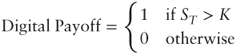
In its American version, which is more uncommon, the option pays off $1 as soon as the strike level is hit.
The Black-Scholes price formula for a digital option is simply:
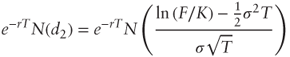
where F is the forward price of S for maturity T, r is the continuous interest rate, and σ is the volatility parameter. When there is an implied volatility smile this formula is inaccurate and a corrective term must be added (see Section 2-1.3).
Digital options are not easy to dynamically hedge because their delta can become very large near maturity. Exotic traders tend to overhedge them with a tight call spread whose range may be determined according to several possible empirical rules, such as:
- Daily volatility rule: Set the range to match a typical stock price move over one day. For example, if the annual volatility of the underlying stock is 32% annually; that is, 32%/√252 ≈ 2% daily, a digital option struck at $100 would be overhedged with $98–$100 call spreads.
- Normalized liquidity rule: Set the range so that the quantity of call spreads is in line with the market liquidity of call spreads with 5% range. The quantity of call spreads is N/R where N is the quantity of digitals and R is the call spread range. If the tradable quantity of call spreads with range 5% is V, the normalized tradable quantity of call spreads with range R would be V × R / 0.05. Solving for R gives
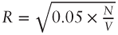 . In practice V is either provided by the option trader or estimated using the daily trading volume of the stock.
1.1.2 Asian Options
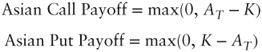
In an Asian call or put, the final underlying asset price is replaced by an average:
where ![]() for a set of pre-agreed fixing dates t1 < t2 <
for a set of pre-agreed fixing dates t1 < t2 < ![]() < tn ≤ T. For example, a one-year at-the-money Asian call on the S&P 500 index with quarterly fixings pays off
< tn ≤ T. For example, a one-year at-the-money Asian call on the S&P 500 index with quarterly fixings pays off ![]() , where S0 is the current spot price and S0.25,…, S1 are the future spot prices observed every three months.
, where S0 is the current spot price and S0.25,…, S1 are the future spot prices observed every three months.
On occasion, the strike may also be replaced by an average, typically over a short initial observation period.
Fixed-strike Asian options are always cheaper than their European counterparts, because AT is less volatile than ST.
There is no closed-form Black-Scholes formula for arithmetic Asian options. However, for geometric Asian options where ![]() , the Black-Scholes formulas may be used with adjusted volatility
, the Black-Scholes formulas may be used with adjusted volatility ![]() and dividend yield
and dividend yield ![]() , as shown in Problem 1.3.3.
, as shown in Problem 1.3.3.
A common numerical approximation for the price of arithmetic Asian options is obtained by fitting a lognormal distribution to the actual risk-neutral moments of AT.
1.1.3 Barrier Options
In a barrier call or put, the underlying asset price must hit, or never hit, a certain barrier level H before maturity:
- For a knock-in option, the underlying must hit the barrier, or else the option pays nothing.
- For a knock-out option, the underlying must never hit the barrier, or else the option pays nothing.
Barrier options are always cheaper than their European counterparts, because their payoff is subject to an additional constraint. On occasion, a fixed cash “rebate” is paid out if the barrier condition is not met.
Similar to digital options, barrier options are not easy to dynamically hedge: their delta can become very large near the barrier level. Exotic traders tend to overhedge them by shifting the barrier a little in their valuation model.
Continuously monitored barrier options have closed-form Black-Scholes formulas, which can be found, for instance, in Hull (2012). The preferred pricing approach is the local volatility model (see Chapter 4).
In practice the barrier is often monitored on a set of pre-agreed fixing dates t1 < t2 < ![]() < tn ≤ T. Monte Carlo simulations are then commonly used for valuation.
< tn ≤ T. Monte Carlo simulations are then commonly used for valuation.
Broadie, Glasserman, and Kou (1997) derived a nice result to switch between continuous and discrete barrier monitoring by shifting the barrier level H by a factor ![]() where β ≈ 0.5826, σ is the underlying volatility, and Δt is the time between two fixing dates.
where β ≈ 0.5826, σ is the underlying volatility, and Δt is the time between two fixing dates.
1.1.4 Lookback Options
A lookback call or put is an option on the maximum or minimum price reached by the underlying asset until maturity:
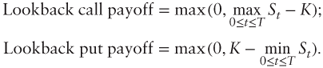
Lookback options are always more expensive than their European counterparts: about twice as much when the strike is nearly at the money, as shown in Problem 1.3.5.
Continuously monitored lookback options have closed-form Black-Scholes formulas, which can be found, for instance, in Hull (2012). The preferred pricing approach is the local volatility model (see Chapter 4).
In practice the maximum or minimum is often monitored on a set of pre-agreed fixing dates t1 < t2 < ![]() < tn ≤ T. Monte Carlo simulations are then commonly used for valuation.
< tn ≤ T. Monte Carlo simulations are then commonly used for valuation.
1.1.5 Forward Start Options
In a forward start option the strike is determined as a percentage k of the spot price on a future start date t0 > 0:
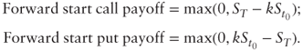
At t = t0 a forward start option becomes a regular option. Note that the forward start feature is not specific to vanilla options and can be added to any exotic option that has a strike.
Forward start options have closed-form Black-Scholes formulas. The preferred pricing approach is to use a stochastic volatility model (see Chapter 4).
1.1.6 Cliquet Options
A cliquet or ratchet option consists of a series of consecutive forward start options, for example:
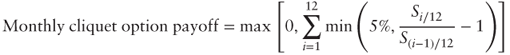
where 5% is the local cap amount. In other words, this particular cliquet option pays off the greater of zero and the sum of monthly returns, each capped at 5%.
Cliquet options can be very difficult to value and especially hedge.
1.2 Multi-Asset Exotics
Multi-asset exotics are based on several underlying stocks or indices, and thus their fair value depends on the level of correlation between the underlying assets. They are typically priced on a Monte Carlo simulation engine with local volatilities (see Chapter 4 and Chapter 6, Section 6-5).
1.2.1 Spread Options
The payoff of a spread option is based on the difference in gross return between two underlying assets:
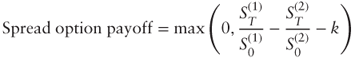
where k is the residual strike level (in %). For example, a spread option on Apple Inc. vs Google Inc. with 5% strike pays off the outperformance of Apple over Google in excess of 5%: if Apple's return is 13% and Google's is 4%, the option pays off 13% − 4% − 5% = 4%.
The value of a spread option is very sensitive to the level of correlation between the two assets. Specifically the option value increases as correlation decreases: the lower the correlation, the wider the two assets are expected to spread apart.
In practice hedging spread options can be difficult because the spread ![]() is often nearly orthogonal to the basket
is often nearly orthogonal to the basket ![]() .
.
When k = 0 a spread option is also known as an exchange option. A closed-form Black-Scholes formula is then available which can be found, for instance, in Hull (2012).
1.2.2 Basket Options
A basket call or put is an option on the gross return of a portfolio of n underlying assets:
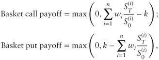
where the weights w1,…, wn sum to 100% and the strike k is expressed as a percentage (e.g., 100% for at the money).
The value of a basket option is sensitive to the level of pairwise correlations between the assets. The lower the correlation, the less volatile the portfolio and the cheaper the basket option.
Basket options do not have closed-form Black-Scholes formulas. A common approximation technique is to fit a lognormal distribution to the actual moments of the basket and then use formulas for the single-asset case.
1.2.3 Worst-Of and Best-Of Options
A worst-of call or put is an option on the lowest gross return between n underlying assets:
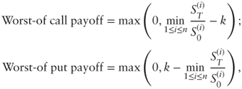
where the strike k is expressed as a percentage (e.g., 100% for at the money). For example, a worst-of at-the-money call on Apple, Google, and Microsoft pays off the worst stock return between the three companies, if positive.
Similarly, a best-of call or put is an option on the highest gross return between n underlying assets.
Worst-of calls and best-of puts are always cheaper than any of their single-asset European counterparts, while best-of calls and worst-of puts are always more expensive.
1.2.4 Quanto Options
The payoff of a quanto option is paid out in a different currency from the underlying assets, at a guaranteed exchange rate. For example, a call on the S&P 500 index quanto euro pays off max(0, ST − K) in euros instead of dollars, thereby guaranteeing an exchange rate of 1 euro per dollar.
The actual exchange rate between the asset currency and the quanto currency is in fact an implicit additional underlying asset. The value of quanto options is very sensitive to the correlation between the primary asset and the implicit exchange rate.
Quanto options are an example of hybrid exotic options involving different asset classes—here equity and foreign exchange.
In terms of pricing, the quanto feature is often approached using a technique called change of numeraire. In summary, this technique says that the risk-neutral dynamics of an asset quantoed in a different currency from its natural currency has the same volatility coefficient but an adjusted drift coefficient.
1.3 Structured Products
Structured products combine several securities together, especially exotic options. They are typically sold as equity-linked notes (ELN) or mutual funds to small investors as well as large institutions. These notes and funds are sometimes traded on exchanges.
In the Capital Guaranteed Performance Note, investors are guaranteed1 to get their $10 mn capital back after five years. This is much safer than a direct $10 mn investment in the S&P 500 index, which could result in a loss. In exchange for this protection, investors receive a smaller share in the S&P 500 performance: 50% instead of 100%.
In the Reverse Convertible Note, investors may lose on their €2 mn capital if Kroger Co. ever trades below the 70% barrier, but never more than a direct investment in the stock (ignoring dividends). Otherwise, investors receive at least €2.3 mn after three years, and never less than a direct investment in the stock (again, ignoring dividends).
In some cases it is possible to break down a structured product into a portfolio of securities whose prices are known and find its value. In all other cases the payoff is typically programmed on a Monte Carlo simulation engine.
Multi-asset structured products significantly expand the payoff possibilities of exotic options. They allow investors to play on correlation and express complex investment views.
Multi-asset structured product valuation is almost always done using Monte Carlo simulations. Hedging correlation risk is often difficult or expensive, and exotic trading desks tend to accumulate large exposures, which can cause significant losses during a market crash.
References
- Baxter, Martin, and Andrew Rennie. 1996. Financial Calculus: An Introduction to Derivative Pricing. New York: Cambridge University Press.
- Broadie, Mark, Paul Glasserman, and Steven Kou. 1997. “A Continuity Correction for Discrete Barrier Options.” Mathematical Finance 7 (4): 325–348.
- Hull, John C. 2012. Option, Futures, and Other Derivatives, 8th ed. New York: Prentice Hall.
Problems
1.1 “Free” Option
Consider a European call option on an underlying asset S with strike K and maturity T where “you only pay the premium if you win,” that is, if ST > K.
- Draw the diagram of the net P&L of this “free” option at maturity. Is it really “free”?
- Find a replicating portfolio for the “free” option using vanilla and exotic options.
- Calculate the fair value of the “free” option premium using the Black-Scholes model with 20% volatility, S0 = K = $100, one-year maturity, zero interest and dividend rates.
1.2 Autocallable
Consider an exotic option expiring in one, two, or three years on an underlying asset S with the following payoff mechanism:
- If after one year S1 > S0 the option pays off 1 + C and terminates;
- Else if after two years S2 > S0 the option pays off 1 + 2C and terminates;
- Else if after three years S3 > 0.7 × S0 the option pays off
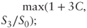
- Otherwise, the option pays off S3/S0.
Assuming S0 = $100, zero interest and dividend rates, and 25% volatility, estimate the level of C so that the option is worth 1 using Monte Carlo simulations.
1.3 Geometric Asian Option
Consider a geometric Asian option on an underlying S with payoff f(AT) where ![]() . Assume that S follows a geometric Brownian motion with parameters (r − q, σ) under the risk-neutral measure.
. Assume that S follows a geometric Brownian motion with parameters (r − q, σ) under the risk-neutral measure.
- Using the Ito-Doeblin theorem, show that
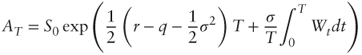
- Using the Ito-Doeblin theorem, show that
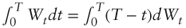 . What is the distribution of this quantity?
 - Show that AT is lognormally distributed with parameters

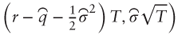 where
where  and
and 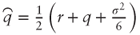 .
.
1.4 Change of Measure
In the context of Appendix 1.A, verify that ![]() using the expression for d
using the expression for d![]() /d
/d![]() .
.
1.5 At-the-Money Lookback Options
The Black-Scholes closed-form formula for an at-the-money lookback call is given as:
where ![]() and
and ![]() .
.
Using a first-order Taylor expansion of the cumulative normal distribution N(·) show that for reasonable rates and maturities we have the proxy:
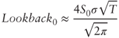
which is twice as much as the European call proxy: ![]() .
.
1.6 Siegel's Paradox
This problem is about foreign exchange rates and goes beyond the scope of equity derivatives.
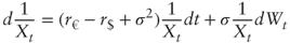
Consider two currencies, say dollars and euros, and suppose that their corresponding interest rates, r$ and r€, are constant. Let X be the euro–dollar exchange rate defined as the number of dollars per euro. The traditional risk-neutral process for X is thus:
where W is a standard Brownian motion.
- Using the Ito-Doeblin theorem, show that the risk-neutral dynamics for the dollar-euro exchange rate, that is, the number 1/X of euros per dollar, is:
- Symmetry suggests that the drift of 1/X should be r€ − r$ instead—this is Siegel's paradox. Use your knowledge of quantos (see Section 1.2.4) to resolve the paradox.
Appendix 1.A: Change of Measure and Girsanov's Theorem
Recall that the Black-Scholes model assumes that the underlying asset price process follows a geometric Brownian motion:
where W is a standard Brownian motion under some objective probability measure ![]() , μ is the objective drift coefficient, and σ is the objective volatility coefficient.
, μ is the objective drift coefficient, and σ is the objective volatility coefficient.
However, the drift coefficient μ disappears from option pricing equations as a result of delta-hedging, and option prices may equivalently be calculated as discounted expected payoffs under a special probability measure ![]() called risk-neutral. Under
called risk-neutral. Under ![]() , the underlying asset price process follows the geometric Brownian motion:
, the underlying asset price process follows the geometric Brownian motion:
where W′ is a standard Brownian motion under ![]() , r is the continuous interest rate, and σ is the same volatility coefficient.
, r is the continuous interest rate, and σ is the same volatility coefficient.
To understand how ![]() and
and ![]() relate, consider the undiscounted expected payoff:
relate, consider the undiscounted expected payoff:
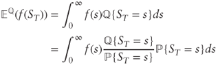
If we define the ratio of densities ![]() then we can write:
then we can write:
The change of measure from ![]() to
to ![]() is thus equivalent to multiplying by the random variable h(ST) called a Radon-Nikodym derivative and properly denoted
is thus equivalent to multiplying by the random variable h(ST) called a Radon-Nikodym derivative and properly denoted ![]() . Girsanov's theorem states that
. Girsanov's theorem states that ![]() exists and is properly defined by a Radon-Nikodym derivative of the form:
exists and is properly defined by a Radon-Nikodym derivative of the form:
Furthermore, ![]() is then a Brownian motion under
is then a Brownian motion under ![]() . Problem 1.3.4 verifies that
. Problem 1.3.4 verifies that ![]() .
.
For a rigorous yet accessible exposition of the change of measure technique and Girsanov's theorem we refer the reader to Baxter and Rennie (1996).