
Chapter 8
Local Correlation
Local correlation models are a recent cutting-edge development in derivatives modeling and extend the concept of local volatility to multiple assets. Indeed if the volatility of each asset is thought to depend on time and the spot price, then the same idea should probably apply to the correlation coefficient between any two assets. However there are theoretical and practical issues: on the theoretical side the entire correlation matrix must remain positive-definite, which can be challenging; and on the practical side there are very few observable basket option prices to calibrate to. In this chapter we give evidence of non-constant implied correlation and introduce a model that is consistent with this behavior.
8.1 The Implied Correlation Smile and Its Consequences
Just as there is an implied volatility smile for options on single stocks, there is also an implied volatility smile for basket options, which is best observed on index options. Figure 8.1 compares the six-month smile on the EuroStoxx 50 index versus the average six-month smile on its constituents. We can see that the slope of the index smile is different from the slope of the constituents' smile, a phenomenon that may only be reproduced by having a different correlation parameter for each moneyness level.
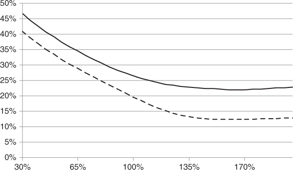
Figure 8.1 Six-month smile on the Dow Jones EuroStoxx 50 index versus the average six-month smile on its 50 constituents as of April 30, 2013.
Data source: OptionMetrics.
Specifically, for fixed maturity T, we may extract the implied correlation curve by means of the formula:

where σ*'s are implied volatilities, w's are basket weights, and k is the moneyness level.
Figure 8.2 shows the implied correlation smile obtained on the Dow Jones EuroStoxx 50 index. We can see that the shape is downward sloping, which is consistent with the intuition that when markets go down correlation goes up.
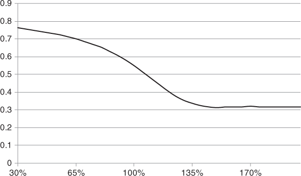
Figure 8.2 Six-month implied correlation on the Dow Jones EuroStoxx 50 index as of April 30, 2013.
This phenomenon suggests that the constant correlation assumption often used to price basket exotics is not correct, opening the way for yet more sophisticated models. This particularly affects the pricing of worst-of and best-of options, which are very sensitive to the level of input correlation.
8.2 Local Volatility with Local Correlation
A local volatility model with local correlation (LVLC) allows the pairwise correlation coefficients to depend on time and spot prices:

and
where ![]() is the local volatility function for asset S(i) (see Chapter 4) and
is the local volatility function for asset S(i) (see Chapter 4) and ![]() is a local correlation function for assets S(i) and S(j).
is a local correlation function for assets S(i) and S(j).
There are many ways to specify the n(n–1)/2 local correlation functions ![]() and in fact some authors let them depend on the entire vector of spot prices
and in fact some authors let them depend on the entire vector of spot prices ![]() . The key practical difficulty here is to ensure that the local correlation matrices
. The key practical difficulty here is to ensure that the local correlation matrices ![]() are positive-definite at all times and across all spot levels.
are positive-definite at all times and across all spot levels.
It is worth nothing that the arbitrage argument leading to a pricing equation for basket options still holds in the case of LVLC models.
When delta-hedging using an LVLC model, the mismatch between the option payoff and the proceeds of the delta-hedging strategy involves n(n + 1)/2 terms corresponding to the gammas and cross-gammas. In the two-asset case with zero interest rates the P&L expression is:

where ![]() and
and ![]() . We can see that correlation (actually covariance) only appears in the cross-gamma term, and thus the only way to eliminate correlation exposure is by dynamically trading another basket option.
. We can see that correlation (actually covariance) only appears in the cross-gamma term, and thus the only way to eliminate correlation exposure is by dynamically trading another basket option.
In practice, exotic option traders tend to mitigate their risk by gamma-hedging their exotic position using single-stock listed vanilla options, but they typically do not cross-gamma-hedge with basket options because these are too illiquid and expensive.
8.3 Dynamic Local Correlation Models
Langnau (2010) and Reghai (2010) both explored a class of LVLC models where local correlations fluctuate between two given “up” and “down” correlation matrices U and D through the convex combination1:
where 0 ≤ α ≤ 1. It is easy to verify that if D and U are positive-definite then so is R.
Langnau shows that if the basket local volatility function ![]() is known, then α is uniquely determined. Specifically, Langnau argues that, subject to certain arbitrage conditions, we must have:
is known, then α is uniquely determined. Specifically, Langnau argues that, subject to certain arbitrage conditions, we must have:
where ![]() is the basket price. Substituting Equation (8.1) and solving for α we obtain:
is the basket price. Substituting Equation (8.1) and solving for α we obtain:

where ![]() for any matrix A = (ai,j). Note that
for any matrix A = (ai,j). Note that ![]() for the vector x with entries
for the vector x with entries ![]() .
.
Langnau's dynamic local correlation model reproduces the index smile very accurately as shown in Figure 8.3 and as such constitutes a significant advance in basket option pricing. In particular, it correctly prices basket variance swaps (without producing a correct hedging strategy).
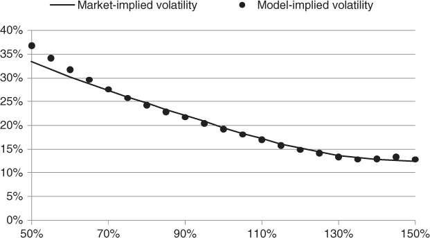
Figure 8.3 The dynamic local correlation model reproduces the one-year Dow Jones EuroStoxx 50 index smile as of April 30, 2013, very accurately.
Data source: OptionMetrics.
8.4 Limitations
The LVLC approach will satisfactorily price a wide range of basket exotics and yield more accurate hedge ratios than the traditional LVCC approach. However, it will not generate realistic implied volatility and correlation smile dynamics for basket cliquet options, for example, for which a stochastic volatility and correlation model would be required.
Additionally the LVLC approach will not produce a meaningful hedging strategy for new generation payoffs such as correlation swaps.
References
- Langnau, Alex. 2010. “A Dynamic Model for Correlation.” Risk Magazine (April): 74–78.
- Reghai, Adil. 2010. “Breaking Correlation Breaks.” Risk Magazine (October): 90–95.
Problems
8.1 Implied Correlation
Consider a stock index made of n constituent stocks with fixed weights w1,…, wn. For fixed maturity T, let a(k) denote the implied volatility of the index at moneyness k, and b(k) denote the average implied volatility of the constituent stocks at moneyness k. Show that implied correlation ![]() is constant if and only if the percentage slopes of a and b are equal (i.e., a′/a = b′/b).
is constant if and only if the percentage slopes of a and b are equal (i.e., a′/a = b′/b).
8.2 Dynamic Local Correlation I
Consider Langnau's dynamic local correlation model with D = I and U = eeT, where I is the identity matrix and e is the vector of 1's. Show that  for a particular choice of nonnegative weights x summing to 1, and then argue that α = ρ(x) where ρ(x) is defined in Equation (6.1).
8.3 Dynamic Local Correlation II
This is a continuation of Problem 2.
Assume for ease of implementation that:
- The Dow Jones EuroStoxx 50 index is made of 50 equally weighted constituent stocks
- Interest and dividend rates are zero
- All implied volatility surfaces have the following parametric form

where k = K/S is moneyness, θ > 0, −1 ≤ ρ ≤ 1, λ ≥ 0.5 are time-independent parameters and:
Download the parameters for the index and its constituents from www.wiley.com/go/bossu and then implement Langnau's dynamic local correlation model with D = I and U = eeT to price one-year arbitrary basket payoffs using 252 time steps. Reproduce Figure 8.3 and then verify that the price of a 50% worst-of call on the 50 constituents is approximately 11.3%.
Hint: You will need to compute time-dependent local volatilities using Equation (4.2).