
Chapter 9
Stochastic Correlation
Stochastic correlation models may provide a more realistic approach to the pricing and hedging of certain types of exotic derivatives, such as worst-of and best-of options and correlation swaps and correlation options. In this chapter, we review various types of stochastic correlation models and propose a framework for the pricing of realized correlation derivatives that is consistent with variance swap markets.
9.1 Stochastic Single Correlation
Consider the following general model framework for two assets S(1) and S(2):

where μ's are instant drift coefficients, σ's are instant volatility coefficients, and ρ is the instant correlation coefficient between the driving Brownian motions W's. Here all the coefficients may be stochastic, and we focus on ρ.
There are some simple ways to make ρ stochastic and comprised between −1 and 1; for example, take ![]() where Z is an independent Brownian motion. The dynamics of dρt may then be found by means of the Ito-Doeblin theorem. One issue with this approach is that the parameters may not be very intuitive.
where Z is an independent Brownian motion. The dynamics of dρt may then be found by means of the Ito-Doeblin theorem. One issue with this approach is that the parameters may not be very intuitive.
A better approach is to specify diffusion dynamics for ρ and examine the Feller conditions at bounds −1 and 1 (see Section 2.4.2.2). A popular process here is the affine Jacobi process, also known as a Fischer-Wright process, which is very similar to Heston's stochastic volatility process (see Section 2.4.2.2):
where ![]() is the long-term mean, κ is the mean reversion speed, and α is the volatility of instant correlation. The Feller condition is then
is the long-term mean, κ is the mean reversion speed, and α is the volatility of instant correlation. The Feller condition is then ![]() . A technical analysis of this type of process can be found in van Emmerich (2006).
. A technical analysis of this type of process can be found in van Emmerich (2006).
Figure 9.1 shows the path obtained for an affine Jacobi process with parameters ![]() . Observe how all values are comprised between −1 and 1.
. Observe how all values are comprised between −1 and 1.

Figure 9.1 Sample path of an affine Jacobi process with parameters  .
.
9.2 Stochastic Average Correlation
We now shift our focus to average correlation measures  as introduced in Section 6.3. Because the correlation matrix
 ![]() must be positive-definite at all times we cannot naively extend the single correlation case with, for instance, n(n − 1)/2 affine Jacobi processes and take their average. Note that as a consequence of positive-definiteness ρ(x) is actually comprised between 0 and 1 for large n.
must be positive-definite at all times we cannot naively extend the single correlation case with, for instance, n(n − 1)/2 affine Jacobi processes and take their average. Note that as a consequence of positive-definiteness ρ(x) is actually comprised between 0 and 1 for large n.
Before we go into further detail we must distinguish between nontradable correlation, such as rolling historical or implied correlations, and tradable correlation, such as the historical correlation observed over a fixed time period [0, T]:
- Nontradable average correlation can be modeled quite freely, using, for example, a standard Jacobi process between 0 and 1 or econometric processes such as Constant and Dynamic Conditional Correlation models (see, e.g., Engle (2009)).
- Tradable average correlation requires special consideration to be consistent with other related securities such as variance swaps.
The rest of this section is devoted to the study of tradable average correlation.
9.2.1 Tradable Average Correlation
Consider ![]() which was introduced in Section 7-1.2 and is related to the proxy formula
which was introduced in Section 7-1.2 and is related to the proxy formula ![]() introduced in Section 6.3.1. Because
introduced in Section 6.3.1. Because ![]() is the ratio of two tradable assets—namely, basket variance and average constituent variance—we can derive its dynamics from those of the two tradable assets. For example, suppose we have:
is the ratio of two tradable assets—namely, basket variance and average constituent variance—we can derive its dynamics from those of the two tradable assets. For example, suppose we have:

where Xt is the price of basket variance at time t, Yt ≥ Xt is the price of average constituent variance at time t, and the driving Brownian motions W, Z are taken under the forward-neutral measure.
Using the Ito-Doeblin theorem the resulting dynamics for ![]() are then:
are then:
where B is another standard Brownian motion constructed from W and Z.
Note that, as the ratio of two prices, ![]() is not the price of correlation at time t, which is why the drift coefficient in Equation (9.1) is nonzero under the forward-neutral measure:
is not the price of correlation at time t, which is why the drift coefficient in Equation (9.1) is nonzero under the forward-neutral measure:
Because ![]() is invariant when multiplying X and Y by the same scalar λ, we may further focus on one-dimensional reductions of the model (see Section 7-2.3) and assume that f, g, h are functions of X/Y:
is invariant when multiplying X and Y by the same scalar λ, we may further focus on one-dimensional reductions of the model (see Section 7-2.3) and assume that f, g, h are functions of X/Y:

In this case Equation (9.1) becomes one-dimensional; that is, the drift and volatility coefficients depend only on time and ![]() . This makes the following Feller analysis considerably easier.
. This makes the following Feller analysis considerably easier.
Omitting the time subscript for ease of exposure and using x to denote the state variable we may rewrite Equation (9.1) as:
The Feller conditions at bounds 0 and 1 are then:

Dividing both the numerator and denominator by g2(u), the integrand in s(y) may be rewritten as ![]() with
with ![]() . Furthermore,
. Furthermore,
- As x → 0 a sufficient condition is that
 in which case we have
  for y0 and y close to 0, and thus
  . A formal proof of sufficiency is proposed in Appendix 9.A.
 - As x → 1 a necessary condition is that s(y) → ∞, which in turn implies that
 diverges (see Appendix 9.B for a formal proof). An analysis of this quantity over the domain p ≥ 0 and | h | ≤ 1 reveals that the only singularity is at (1, 1). Thus, as a corollary we have the weak necessary condition
  and h(u) → 1 as u → 1. This configuration intuitively makes sense: if average correlation is close to 1, there is almost no diversification effect, and basket variance and average constituent variance become almost identical.
Additionally, we want f ≥ g because basket variance is more volatile than average constituent variance, which unfortunately makes the sufficient condition stated above ineffective, since p ≥ 1. We must keep all these properties in mind when researching suitable functions f, g, and h.
9.2.2 The B-O Model
The following model, which we call the B-O model (for beta-omega), is a further step towards a suitable stochastic average correlation model:

where ω is the instant volatility of constituent volatility and β is the “additional” volatility of basket volatility.1 The corresponding dynamics for the average correlation ![]() are then given by Equation (9.2) using the functions:
are then given by Equation (9.2) using the functions:

Unfortunately, both lower and upper bounds [0,1] turn out to be attracting in the B-O model, making it unsuitable for extreme starting values ρ0 and long-term horizons T. However, empirical simulations exhibit plausible paths. Further research is needed here.
Figure 9.2 shows 10 sample paths obtained with parameters ω = 70%, β = 40% and ![]() . Remarkably enough, using Monte Carlo simulations the price of correlation
. Remarkably enough, using Monte Carlo simulations the price of correlation ![]() in this model appears to be close to the initial value
in this model appears to be close to the initial value ![]() , also known as variance-implied correlation. This suggests that the fair strike of a correlation swap on
, also known as variance-implied correlation. This suggests that the fair strike of a correlation swap on ![]() should be close to
should be close to ![]() , and by extension a similar result should apply to standard correlation swaps.
, and by extension a similar result should apply to standard correlation swaps.
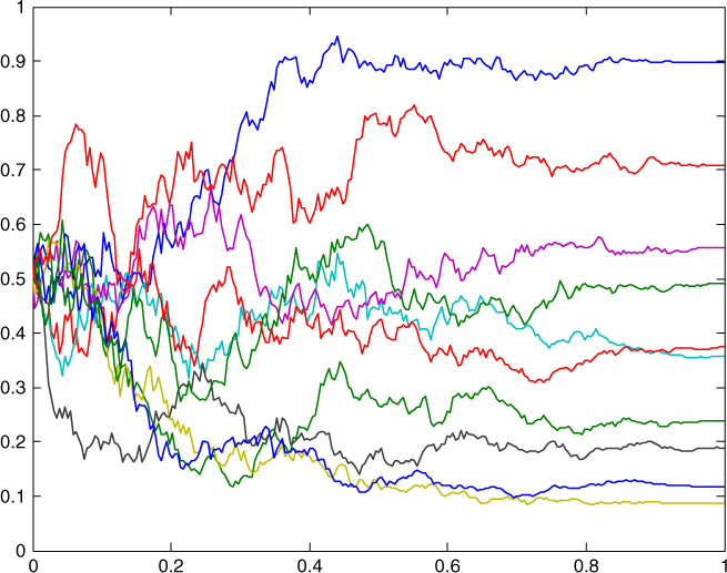
Figure 9.2 Ten sample paths using the B-O model with parameters ω = 70%, β = 40%, and  .
.
9.3 Stochastic Correlation Matrix
A yet more ambitious endeavor is to devise a model for the evolution of the entire correlation matrix ![]() through time. As pointed out earlier, the difficulty here is to ensure that Rt is positive-definite at all times.
through time. As pointed out earlier, the difficulty here is to ensure that Rt is positive-definite at all times.
It is worth emphasizing that, when correlations are tradable, we should also ensure that the induced dynamics of average correlation ![]() be consistent with variance swaps under the forward-neutral measure.
be consistent with variance swaps under the forward-neutral measure.
As already pointed out in Section 6.2, equity correlation matrices have structure—namely, there is typically one large eigenvalue dominating all others, and the associated eigenvector corresponds to an all-stock portfolio. As such an equity correlation matrix cannot be viewed as any kind of random matrix.
Here we need to be more specific about the meaning of a (symmetric) random matrix. This concept was first introduced by Wishart (1928) in the form M = XXT where X is an n × n matrix of independent and identically distributed random variables; the special case where X is Gaussian deserves particular attention since it tends to the identity matrix as n → ∞. Another approach is Wigner's, whereby ![]() ; a remarkable property is that the empirical distribution of ordered eigenvalues then follows the semi-circle law:
; a remarkable property is that the empirical distribution of ordered eigenvalues then follows the semi-circle law:
9.3.1 Spectral Decomposition and the Common Factor Model
The empirical analysis of equity correlation matrices suggests that they may be viewed as the sum of a (truly) random matrix and an orthogonal projector onto the maximal eigenvector. Following the spectral theorem we may indeed write:

where (v1,…, vn) is an orthonormal basis of eigenvectors with eigenvalues λ1 ≤ ![]() ≤ λn. The residual matrix
≤ λn. The residual matrix ![]() may then be approximated by a Wishart-type matrix.
may then be approximated by a Wishart-type matrix.
For large n we could ignore ![]() altogether and write:
altogether and write:

where a1,…, an are the entries of the maximal eigenvector vn and ![]() . Note that
. Note that ![]() has different eigenelements from R; however, λn is related to average correlation because
has different eigenelements from R; however, λn is related to average correlation because ![]() as n → ∞.
as n → ∞.
This approach corroborates Boortz's Common Factor Model (2008) whereby:

where (ξt,1,…, ξt,n) is a vector of correlated stochastic processes in (−1, 1), such as affine Jacobi processes. One issue with the Common Factor Model is that the (equally weighted) average realized correlation has a risk-neutral drift, which has no particular reason to fit in the framework of Section 9.2.1. In other words the Common Factor Model does not appear to be consistent with variance swap markets.
9.3.2 The  Fischer-Wright Model
Recent work by Ahdida and Alfonsi (2012) alternatively proposes the following stochastic process for the correlation matrix Rt, which is a generalization of the Jacobi process:

where the matrix ![]() is the long-term correlation mean,
is the long-term correlation mean, ![]() is a diagonal matrix of mean-reversion speeds, α = diag(α1,…, αn) is a diagonal matrix of volatility coefficients,
is a diagonal matrix of mean-reversion speeds, α = diag(α1,…, αn) is a diagonal matrix of volatility coefficients, ![]() is the diagonal matrix with coefficient 1 at position (i,i) and 0 elsewhere,
is the diagonal matrix with coefficient 1 at position (i,i) and 0 elsewhere, ![]() denotes the unique square root of a positive-semidefinite matrix H, and (Wt) is an n × n matrix of independent standard Brownian motions.
denotes the unique square root of a positive-semidefinite matrix H, and (Wt) is an n × n matrix of independent standard Brownian motions.
Subject to the condition ![]() being positive-semidefinite, the Ahdida-Alfonsi process is guaranteed to remain a valid correlation matrix through time; however, a corrected Euler scheme is required for simulation.
being positive-semidefinite, the Ahdida-Alfonsi process is guaranteed to remain a valid correlation matrix through time; however, a corrected Euler scheme is required for simulation.
Unfortunately, Ahdida and Alfonsi have not studied the eigenelements of their respective correlation matrix processes. and it is difficult to tell how realistic their model is within the realm of equity correlation matrices. In particular, there is no guarantee that the induced dynamics of average correlation can be made consistent with realistic dynamics of basket variance and average constituent variance in the fashion described early in the chapter. Further research is thus needed.
References
- Ahdida, Abdelkoddousse, and Aurélien Alfonsi. 2012. “A Mean-Reverting SDE on Correlation Matrices.” arXiv:1108.5264.
- Boortz, C. Kaya. 2008. “Modelling Correlation Risk.” Diplomarbeit preprint, Institut für Mathematik, Technische Universität Berlin & Quantitative Products Laboratory, Deutsche Bank AG.
- Engle, Robert. 2009. Anticipating Correlations: A New Paradigm for Risk Management. Princeton, NJ: Princeton University Press.
- van Emmerich, Cathrin. 2006. “Modelling Correlation as a Stochastic Process.” Bergische Universität Wuppertal. Preprint.
- Wishart, John. 1928. “The Generalised Product Moment Distribution in Samples from a Normal Multivariate Population.” Biometrika 20A (1–2): 32–52.
Problems
Consider a stock S, which does not pay dividends, with dollar price S$, and let X be the exchange rate of one dollar into euros. Assume that S$ and X both follow geometric Brownian motions under the dollar risk-neutral measure with joint dynamics:

where r$ is the constant dollar interest rate, σ, ν and η are free constant parameters, and W, Z are standard Brownian motions with stochastic correlation ![]() .
.
- Show that the forward price of S quanto euro for maturity T is
 .
. - Assume that S0$ = $100, r$ = 0, σ = 25%, η = 10%,
 with
with  . Compute the one-year forward price of S quanto euro using Monte Carlo simulations over 252 trading days. Answer: €100.60
Consider the model for stochastic average correlation:

- Verify that the process remains within (0,1) and that the lower bound is non-attracting.
- Define
 . Find f(x), g(x) such that
  satisfies Equation (9.2). Hint: Show that
  where p = f/g and solve for p.
 - Do you think that this model is suitable?
Appendix 9.A: Sufficient Condition for Lower Bound Unattainability
Following the notations of Section 9.2.1, suppose that ![]() . By the definition of a limit this means that for arbitrary ϵ > 0 there exists an α > 0 such that:
. By the definition of a limit this means that for arbitrary ϵ > 0 there exists an α > 0 such that:
Thus, for all 0 < u ≤ α, ![]() . By integration over [y0, y] ⊂ [0, α] we get:
. By integration over [y0, y] ⊂ [0, α] we get:

Taking exponentials:
and thus ![]() since
since ![]() diverges for any β ≥ 0.
diverges for any β ≥ 0.
Appendix 9.B: Necessary Condition for Upper Bound Unattainability
Suppose that ![]() converges to a finite limit
converges to a finite limit ![]() . By the definition of a limit this means that for arbitrary ϵ > 0 there exists an α < 1 such that:
. By the definition of a limit this means that for arbitrary ϵ > 0 there exists an α < 1 such that:
Thus, for all α ≤ u ≤ 1, ![]() . By integration over [y0, y] ⊂ [α, 1] we get:
. By integration over [y0, y] ⊂ [α, 1] we get:
Taking exponentials:
and thus ![]() is finite since
is finite since ![]() converges for any β, thereby contradicting the requirement that
converges for any β, thereby contradicting the requirement that ![]() .
.