Chapter 7
Correlation Trading
With the development of multiasset exotic products it became possible, and at times necessary, to trade correlation more or less directly. The first correlation trades were actually dispersion trades where a long or short position on a multi-asset option is offset by a reverse position on single-asset options. Recently pure correlation trades appeared in the form of correlation swaps.
7.1 Dispersion Trading
The payoff of a dispersion trade is of the form:
where β is an arbitrary coefficient or leg ratio, which is typically determined so that the trade has zero initial cost, and all other notations are self-explanatory.
The intuition behind dispersion trades is that the basket option's leg provides exposure to volatility and correlation. To isolate the correlation exposure, it is necessary to hedge, if only approximately, the volatility exposure: this is precisely the purpose of the short single options' leg.
The two most popular types of dispersion trades are vanilla dispersions, based on vanilla options (typically straddles), and variance dispersions, based on variance swaps.
7.1.1 Vanilla Dispersion Trades
The payoff formula for a vanilla dispersion trade on a selection of n stocks S(1),…, S(n) with weights w1,…, wn is given as:
where β is the leg ratio, T is the maturity, and k is the moneyness level (strike/spot).
The trade cost is 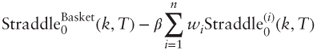 , and the leg ratio for a zero-cost trade is thus
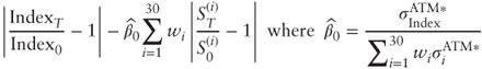
 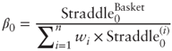 . In the case of short-term near-the-money forward straddles, we have the proxy
 ![]() where σ*'s are at-the-money implied volatilities and ρ*ATM is at-the-money average implied correlation (see Problem 7.1).
where σ*'s are at-the-money implied volatilities and ρ*ATM is at-the-money average implied correlation (see Problem 7.1).
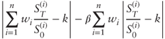
From a trading perspective, vanilla dispersion trades are attractive because they tend to be liquid, cost-effective, and customizable. However, a major disadvantage is that they need to be delta-hedged; furthermore, the delta-hedging profit and loss (P&L) involves the gammas of n + 1 options and is only very loosely connected to correlation:
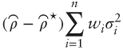
- Assuming constant implied volatility and zero interest rates, the total delta-hedging P&L for option i (where i = Basket or 1,…, n) is:
where ![]() is the option's dollar gamma at time t, σt,i is the instantaneous volatility of asset S(i) at time t, and
is the option's dollar gamma at time t, σt,i is the instantaneous volatility of asset S(i) at time t, and ![]() is implied volatility.
is implied volatility.
- The total delta-hedging P&L of the dispersion trade is thus:
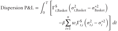
Using the proxy formula from Section 6.3.1 and rearranging terms we can write:
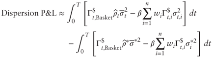
Because the dollar gammas are all different and keep changing, the single option leg will likely be a poorly efficient hedge against the volatility exposure resulting from ![]() .
.
7.1.2 Variance Dispersion Trades
Variance dispersion trades appeared as a spinoff of the expansion of the variance swaps market and offer a much more direct way to trade correlation than vanilla dispersions. Specifically, the payoff formula for a selection of n stocks S(1),…, S(n) with weights w1,…, wn is:
where σ's are realized volatilities between the start date t = 0 and the maturity date t = T and β is the leg ratio. Typically the n stocks are the constituents of an equity index (or a subset), the weights are based on market capitalization at the start date, and σBasket is replaced with the volatility of the index. In practice each realized volatility is capped at a certain level to mitigate volatility “explosions” resulting from bankruptcies, for example.
The trade cost is simply 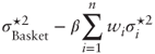 where σ
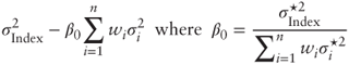
![]() 's are fair variance swap strikes, and thus the leg ratio for a zero-cost trade is
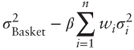
's are fair variance swap strikes, and thus the leg ratio for a zero-cost trade is 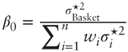 . Note that β0 differs slightly from the correlation proxy formula
 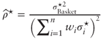 and gives rise to a new average correlation measure:
Note that by Jensen's inequality we must have ![]() . Figure 7.1 shows that
. Figure 7.1 shows that ![]() differ very little in practice, and that they are somewhat above at-the-money implied correlation
differ very little in practice, and that they are somewhat above at-the-money implied correlation ![]() .
.
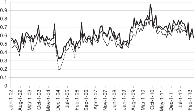
Figure 7.1 Comparison between the six-month implied correlation proxy  (bold line), the six-month variance-based implied correlation
  (dashed line), and at-the-money implied correlation
  (thin line) for the Dow Jones EuroStoxx 50 index.
Data source: OptionMetrics.
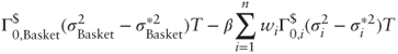
By definition of ![]() we may rewrite the payoff of a zero-cost variance dispersion trade as:
we may rewrite the payoff of a zero-cost variance dispersion trade as:
In other words the P&L on a zero-cost variance dispersion trade is the spread between realized and implied average correlation multiplied by the average realized variance of the constituent stocks. As such the trade will make money when realized correlation exceeds implied correlation, and lose money otherwise—a remarkable property.
From a trading perspective, variance dispersion trades are attractive because there is a persistent gap between implied and realized correlation as shown in Figure 7.2 on the Dow Jones EuroStoxx50 index.
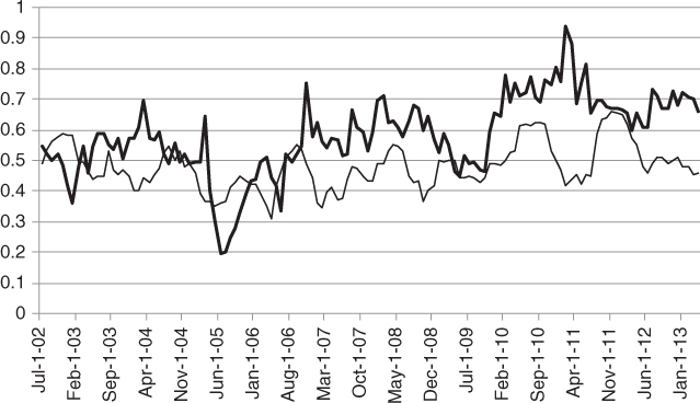
Figure 7.2 Six-month variance-based implied correlation  (bold line) and realized correlation
  six months later (thin line) for the Dow Jones EuroStoxx 50 index.
Data sources: OptionMetrics, Bloomberg.
7.2 Correlation Swaps
7.2.1 Payoff
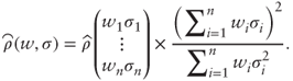
A correlation swap is a forward contract on average realized correlation. Specifically the payoff formula for a selection of n stocks S(1),…, S(n) with weights w1,…, wn is:

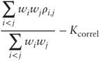
where ρ's are pairwise correlation coefficients observed between the start date t = 0 and the maturity date t = T, and Kcorrel is the strike level between 0 and 1. We recognize the average correlation measure ![]() from Section 6.3.
from Section 6.3.
The main attraction of correlation swaps is that they are pure correlation trades. The main disadvantage is that there is no consensus model to price and hedge them—in particular the strike ![]() trading on the over-the-counter market may significantly differ from average implied correlation measures.
trading on the over-the-counter market may significantly differ from average implied correlation measures.
Correlation swaps are typically offered by investment banks to sophisticated investors on an opportunistic basis to offload the correlation risk accumulated by their exotic trading desks. This is because exotic derivatives sold by banks tend to be long correlation (i.e., their value increases when correlation increases), resulting in large short correlation exposures (i.e., the bank loses money when correlation increases).
7.2.2 Pricing
To approach the pricing of correlation swaps, note that when the stocks are the constituents of an equity index and weights are based on market capitalizations, the average realized correlation measure ![]() is usually close to
is usually close to 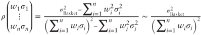 , which itself may be approximated with
 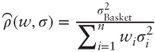 . This suggests that a correlation swap may be approximately priced as a derivative of two tradable assets: basket variance and average constituent variance.
Based on this observation, Bossu (2005) proposed a simple “toy model” to price and hedge correlation swaps, which is a straightforward extension of the Black-Scholes model in the two-asset case. One important theoretical limitation of the toy model is that it is not entirely well-specified and allows average realized correlation to exceed 1 in a small number of paths.
A modified version of the toy model where correlation is constrained between –1 and 1 is derived in Chapter 9. This version is more mathematically satisfying but unfortunately loses the simplicity of the original toy model.
7.2.3 Hedging
While research for the ultimate correlation swap model is still ongoing, we may state certain interesting properties. In general, two-asset models will produce a forward price formula ![]() for correlation where Xt, Yt are the forward prices at time t of
for correlation where Xt, Yt are the forward prices at time t of ![]() respectively (in particular
respectively (in particular ![]() , and
, and ![]() ). The hedge ratios are then given as
). The hedge ratios are then given as ![]() as usual.
as usual.
Because ![]() under the forward-neutral measure and because XT/YT is invariant when multiplying XT and YT by the same scalar λ, we must also have
under the forward-neutral measure and because XT/YT is invariant when multiplying XT and YT by the same scalar λ, we must also have ![]() and thus there exists a unique pricing function g such that
and thus there exists a unique pricing function g such that ![]() which is the one-dimensional reduction of the two-asset model f. In this case the hedge ratios are given as
which is the one-dimensional reduction of the two-asset model f. In this case the hedge ratios are given as ![]() where
where ![]() . Remarkably enough the corresponding hedge is then a zero-cost variance dispersion with leg ratio
. Remarkably enough the corresponding hedge is then a zero-cost variance dispersion with leg ratio ![]() .
.
This general property shows that the pricing and hedging of correlation swaps is strongly interconnected with variance dispersion trading.
Problems
7.1
Consider a zero-cost vanilla dispersion trade.
- Show that β0 must be comprised between 0 and 1 under penalty of arbitrage.
- Derive the proxy
 for at-the-money-forward straddles.
7.2
- In the Black-Scholes model with zero interest rates, show that the expectation at time 0 of the future dollar gamma of a European option at horizon t is given as:
where Γt is the option's gamma at time t and St is the underlying asset price at time t.
Hint: Use the Black-Scholes partial differential equation and the Ito-Doeblin theorem to show that
 .
. - Consider a vanilla dispersion trade with leg ratio β. Assume zero rates and dividends and that all realized volatilities are constant. Show that the expectation of the total delta-hedging P&L is then:
7.3
Consider a variance dispersion trade with leg ratio β. Show that if  the portfolio is initially vega-neutral (i.e., algebraically insensitive to changes in implied volatility).
7.4
Download the market data for the DAX and its 30 constituents from www.wiley.com/go/bossu and calculate the payoffs of:
- A three-month zero-cost at-the-money vanilla dispersion trade:
- A three-month zero-cost variance dispersion trade
- A three-month correlation swap: