
Solutions Manual
This Solutions Manual includes answers to all of the end of chapter problems found in this book (except for a few coding problems where the numerical answer is provided in the text).
Chapter 1: Exotic Derivatives
1.1 “Free” Option
- The option is not really free because we may end up at a loss at and above the strike price. (See Figure S.1.)
- The replicating portfolio would include selling x digital calls struck at K at price p and buying a vanilla call struck at K for the premium of m. In order for the portfolio to have zero cost we must have
 .
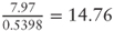
. - The cost of one digital call using the Black-Scholes model with the given parameters is $0.5398. The premium of the vanilla call from the Black-Scholes model is $7.97. Solving for x we get
 .
.
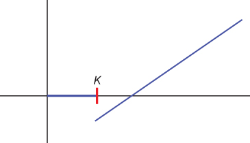
Figure S.1 “Free” option payoff.
1.2 Autocallable
Answer: ![]() .
.
1.3 Geometric Asian Option
- From Ito-Doeblin we have
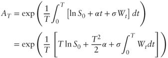
 where α = r − q − ½σ2. Substituting into the definition of AT we get:
- which yields the required expression for AT after simplifications.
- From Ito-Doeblin, we get
 , which yields the required result after integration of both sides over [0, T]. The distribution of
  is thus normal with zero mean and variance
  .
. - Substituting
 and
and  we need to show that ln AT is normally distributed with mean:
- and variance
 . Indeed the mean matches the expression from question (a), and using question (b) we find that the variance of
  is
is 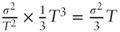 as required.
1.4 Change of Measure
We have ![]() with
with ![]() . Since
. Since ![]() we have after substitution:
we have after substitution:
But ![]() and thus
and thus ![]()
![]() . Expanding the second squared bracket and cancelling terms we are left with
. Expanding the second squared bracket and cancelling terms we are left with ![]() as required.
as required.
1.6 Siegel's Paradox
- Straightforward application of Ito-Doeblin.
- The “risk-neutral” dynamics of 1/X from question (a) correspond to the dollar risk-neutral measure, in which 1/X is non tradable (number of euros per dollar). The paradox is resolved by introducing the euro risk-neutral measure where 1/X follows the process:
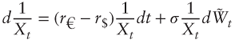
In the dollar risk-neutral measure, 1/X is the price of the dollar-euro exchange rate quanto dollar. Following the notations of Section 1.2.4 and defining S = 1/X, we have ρ = −1 and η = σ; thus the drift of S quanto dollar under the dollar risk-neutral measure is r€ − r$ − ρση = r€ − r$ + σ2 as required.
Chapter 2: The Implied Volatility Surface
2.1 No Call or Put Spread Arbitrage Condition
We know the upper bound is:
and we know that ![]() so after rearranging terms we get:
so after rearranging terms we get:
We know the lower bound is:
and we know that ![]() so we get
so we get
From put-call parity: ![]() , and thus:
, and thus:
Putting them together we get:
Furthermore ![]() and
and ![]()
Thus:
as required.
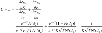
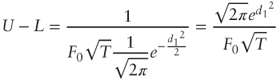
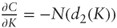
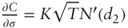
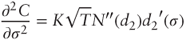
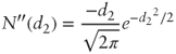
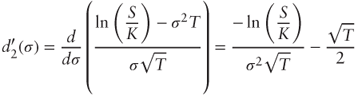
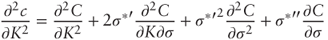
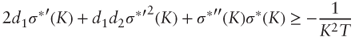
2.2 No Butterfly Spread Arbitrage Condition
- Identities:
- We have:
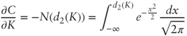
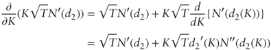
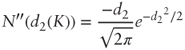
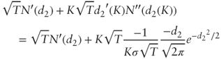
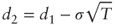
Differentiating with respect to K:
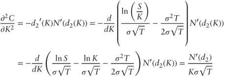
as required.
Differentiating
 with respect to σ:
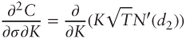
Using the chain rule:
But:
Substituting
 and
and  :
:
Using the fact that
 , we get:
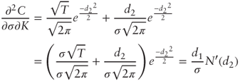
- Differentiating
 with respect to σ:
We have:
and:
Substituting back into
 :
:
Factoring by
 and recognizing d1 we obtain as required:
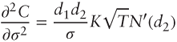
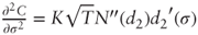
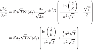
- First-order derivative:
 . Second-order derivative:

- which yields the required result after noting that fxy = fyx by Schwarz's theorem.
- Applying the second-order chain rule:
Substituting the identities from (a) we get the required result after further straightforward algebra.
- After simplifications
 is equivalent to:
2.3 Sticky True Delta Rule
- Applying the chain rule:
 , whence the required result after substituting K = 1 and T = 1.
 - If
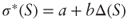 then
then 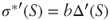 and thus
  yielding the required result after appropriate substitutions.
 - c. Because Δ′ > 0 (call delta goes up as S goes up) and b < 0 (volatility goes down as S and Δ go up) the sticky true delta rule would produce a lower delta than Black-Scholes.
Chapter 3: Implied Distributions
3.1 Overhedging Concave Payoffs
Assume f(K1) = 0 for simplicity. From left to right: start with f′(K1) calls struck at K1 so as to be tangential to the payoff; add ![]() calls struck at K2 such that the portfolio matches the payoff f(K3) at K3; then add
calls struck at K2 such that the portfolio matches the payoff f(K3) at K3; then add ![]() calls struck at K3 so as to be tangential to the payoff after K3; and so on (see Figure S.2).
calls struck at K3 so as to be tangential to the payoff after K3; and so on (see Figure S.2).

Figure S.2 Over-hedging concave payoffs.
3.2 Perfect Hedging with Puts and Calls
From Section 3.2:
Splitting the integral at F and using terminal put-call parity ![]() we get:
we get:
But ![]() , and:
, and:
After substitutions and simplifications we get:
Thus:
because ![]() .
.
3.3 Implied Distribution and Exotic Pricing
-
- Answer: ≈ .1043
- Answer: ≈ 1.0789
- Answer: ≈ .2693
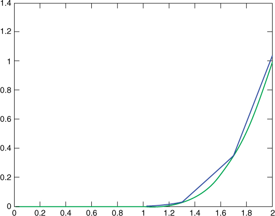
- Answer: ≈ .0211. Vanilla overhedge with strikes 0.5, 0.9, 1, 1.1, 1.3, 1.7: Quantities are 0, 0, 0.0100, 0.1200, 0.6700, and 1.5200 (see Figure S.3).
-
- (i Answer: approximately $0.8965.
- (ii Answer: approximately $0.8626.
3.5 Path-Dependent Payoff
- For example: forward start option, Asian option.
- Pseudo-code:
- Loop for i = 1 to N:
- Generate and calculate
- Generate
 and
and  independently and calculate
- Calculate
- Generate and calculate
- Return
- Loop for i = 1 to N:
- We only know the marginal distributions of
 but we are missing the conditional implied distribution of
  .
.
3.6 Delta
From ![]() we get
we get ![]() and thus:
and thus:
atm_vol = SVI(1);
atm_vol1 = SVI(1/(1+epsilon));
price = 0;
for i=1:n
  normal = randn;
  x = exp(atm_vol*normal*sqrt(T) - 0.5*atm_vol∧2*T);
  x1 = (1+epsilon)*exp(atm_vol1*normal*sqrt(T) − 0.5*atm_vol1∧2*T);
  price = (i-1)/i*price + Payoff(x)*ImpDist(x) …
          / lognpdf(x,-0.5*atm_vol∧2*T,atm_vol*sqrt(T)) / i;
  price1 = (i-1)/i*price1 + Payoff(x1)*ImpDist(x1) …
          / lognpdf(x1,-0.5*atm_vol1∧2*T,atm_vol1*sqrt(T)) / i;
end
delta = price − price1
Chapter 4: Local Volatility and Beyond
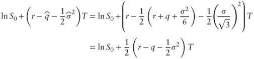
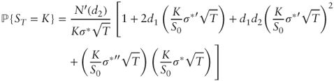
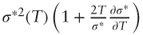
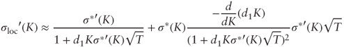
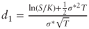
4.1 From Implied to Local Volatility
- We rewrite Equation (4.1) by solving for
 after using the result from Problem 2.4.2(c) for
  .
.
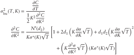
Take
 and derive with respect to T:
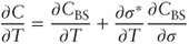
We are given
 and
and  so:
so: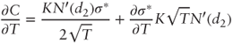
We then plug in
 and
and  into Equation (4.1):
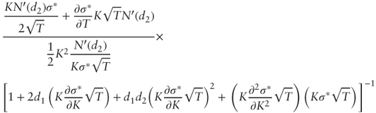
By dividing both numerator and denominator by
 , we obtain the desired Equation (4.2):
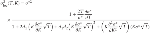
- Replace
 with
with  so we now have:
Now using the Hint:
Thus
 =
=  and by integration we find that:
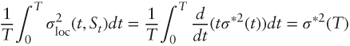
as required.
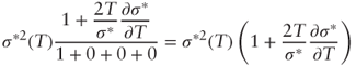
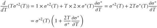
- To establish the hint, note that
 by linearity of σ*, and substitute
 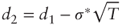 . Differentiating
 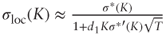 with respect to K we obtain:
Near the money both denominators are close to 1; furthermore
 gives
gives  . After substitution and simplification:
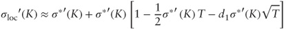
whose leading term is
 .
.
4.2 Market Price of Volatility Risk
- The delta-hedged portfolio Π is long one option and short
 units of S. Thus:
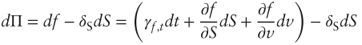
- which yields the required result after cancelling terms.
- We have:
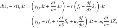
But
 which yields the required result after substitution and simplifications.
 - Conditional expectation:
 . Conditional standard deviation:
Thus
 , that is, at time t the risk-neutral expected return on the delta-hedged portfolio is the risk-free interest rate plus a positive or negative risk premium, which is proportional to the risk of the portfolio, with proportionality coefficient λ. This result applies to any option and λ is independent from the particular option chosen, which is why it is called the market price of volatility risk.
4.3 Local Volatility Pricing
- Figure S.4 shows a graph of the corresponding local volatility surface.
- Using Monte Carlo simulations:
- “Capped quadratic” option:
 ; answer: 0.76949
 - Asian at-the-money-call:
 ; answer: 0.1242
 - Barrier call:
 if S always traded above 80 using 252 daily observations, 0 otherwise. Answer: 12.87577
- “Capped quadratic” option:
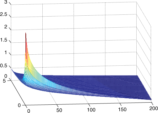
Figure S.4 Local volatility surface.
Chapter 5: Volatility Derivatives
5.1 Delta-Hedging P&L Simulation
- Positive Path: See Figure S.5
Negative Path: See Figure S.5
- Average P&L: −$11,663.80 (see Figure S.6)
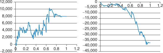
Figure S.5 Cumulative P&L: positive and negative paths.
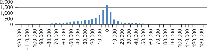
Figure S.6 Distribution of final cumulative P&L.
5.2 Volatility Trading with Options
- (i) If σ is constant then
 . For a vanilla call Γ > 0 and thus the cumulative P&L is always positive.
(ii) We have
 . By iterated expectations:
- The aggregate cumulative P&L is:

As a sum of two independent normal distributions the aggregate distribution is normal with parameters:
- Mean: q1m1 + q2m2
- Standard deviation:
This result sheds light on the diversification effect obtained by delta-hedging several options within an option book: the expected income is the sum of individual delta-hedging P&Ls, but it is less risky than delta-hedging a single position.
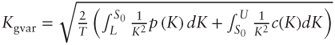
5.4 Generalized Variance Swaps
- From Ito-Doeblin:
 . But
. But  ; rearranging terms we get:
 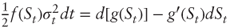 . Integrating over [0, T] yields the desired result.
Thus generalized variance may be replicated by a combination of cash, two derivative contracts paying off g(ST) at maturity, and dynamically trading S to maintain a short position of 2g′(St) at all times. Taking expectations we find that the fair value is:
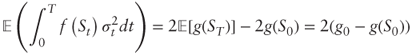
since
 (dWt) = 0.
 - From Problem 3.4.2 we get:

 whence the required formula after substituting
  and annualizing.
 - For the corridor varswap
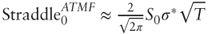
5.5 Call on Realized Variance
- Solving for vt we have:
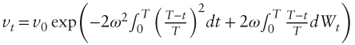 Thus vt is lognormally distributed with mean
 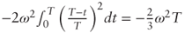 and standard deviation
  . From Black's formula we have
  where
where  . At the money this simplifies to
  which yields the required formula because N(x) − N(−x) = 2N(x) − 1.
 - For x ≈ 0 we have
 .
.
Chapter 6: Introducing Correlation
6.1 Lower Bound for Average Correlation
- Substitute x = e in
 .
. - Because
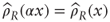 we have
  . Define the Lagrangian
  . The first-order condition yields
  that is,
  . The constraint eTx = 1 then gives the value of λ and we get the required result after substitution and simplification.
 - (i) By spectral decomposition:
 . Furthermore, Parseval's identity states that
  for any x, and thus
  . Scaling by appropriate constants we obtain the required result.
(ii) Rewrite
 and make the approximation that for i = 1,…, n − 1:
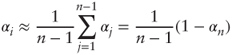
which is justified by the fact that αn ≈ 1 since vn and e are assumed to form a tight angle. Proceed similarly for H.
6.2 Geometric Basket Call
- We have:
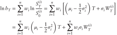
- where
 is the annualized risk-neutral drift of S(i). As a sum of normal variables ln bT is normally distributed with mean
 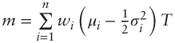 and variance:
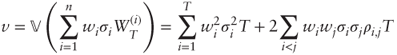
 where
where  . Using Black's formula:
  with
with 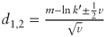 . Further simplifications are possible.
6.4 Continuously Monitored Correlation
After substitution, we have by Cauchy-Schwarz:
where ![]() .
.
Chapter 7: Correlation Trading
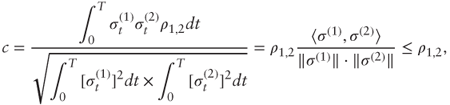
7.1
 is positive because straddles always have a positive payoff and thus price. It must be less than 1 because of the triangle inequality:
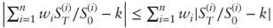
- Use the proxy
7.2
- From the Black-Scholes PDE
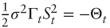 . Applying Ito-Doeblin to Θ:
  . Taking expectations we get:
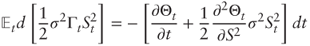
- which vanishes because Greeks must also satisfy the Black-Scholes PDE.
7.3
At time 0 the portfolio value is ![]() , and the vega of each component is
, and the vega of each component is ![]() . Hence the portfolio vega is
. Hence the portfolio vega is ![]() .
.
Chapter 8: Local Correlation
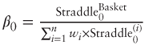
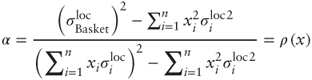
8.1 Implied Correlation
Implied correlation is constant iff ![]() , i.e., iff
, i.e., iff ![]() , whence the required result after simplifications.
, whence the required result after simplifications.
8.2 Dynamic Local Correlation I
When D = I and U = eeT Langnau's alpha is:
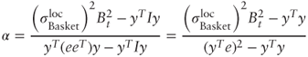
where ![]() . Define
. Define ![]() and divide both the numerator and denominator of the above expression by B to get:
and divide both the numerator and denominator of the above expression by B to get:
It is easy to verify that ![]() .
.
Chapter 9: Stochastic Correlation
9.2
- The process clearly remains within [0,1] because it is continuous and its drift and volatility coefficients vanish at 0 and 1. Let us show that the bound 0 is nonattracting:
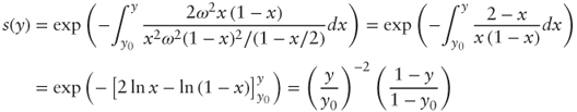
Thus
 since
since  diverges. A similar analysis shows that the bound 1 is also nonattracting.
 - We want to find f(x), g(x) such that:
Thus we must solve:
Taking ratios we get
 ; dividing both numerator and denominator by g2 on the left-hand side we obtain
  . Solving for p after substituting
  we find
  , that is,
  . Substituting in
  and simplifying we get
  , and thus
  .
. - This model is not suitable for several reasons: it has only one parameter ω, which leaves little freedom for parameterization, and the volatility of basket variance f is lower than the volatility of constituent variance g, which is contrary to empirical observation.