Truth be told, you won’t be using object-oriented programming in most day-to-day R programming. Most analyses you do in R involve the transformation of data, typically implemented as some sort of data flow, which is best captured by functional programming. When you write such pipelines, you will probably be using polymorphic functions, but you rarely need to create your own classes. If you need to implement a new statistical model, however, you usually do want to create a new class.
A lot of data analysis requires that you infer parameters of interest or you build a model to predict properties of your data, but in many of those cases, you don’t necessarily need to know exactly how we constructed the model, how it infers parameters, or how it predicts new values. You can use the coefficients function to get inferred parameters from a fitted model, or you can use the predict function to predict new values, and you can use those two functions with almost any statistical model. That is because most models are implemented as classes with implementations for the generic functions coefficients and predict.
As an example of object-oriented programming in action, we can implement our own model in this chapter. We will keep it simple, so we can focus on the programming aspects and not the statistical theory, but still implement something that isn’t already built into R. We will implement a version of Bayesian linear regression.
Bayesian Linear Regression
The simplest form of linear regression fits a line to data points. Imagine we have vectors x and y, and we wish to produce coefficients w[1] and w[2] such that y[i] = w[1] + w[2] x[i] + e[i] where the e is a vector of errors that we want to make as small as possible. We typically assume that the errors are identically normally distributed when we consider it a statistical problem, and so we want to have the minimal variance of the errors. When fitting linear models with the lm function, you get the maximum likelihood values for the weights w[1] and w[2], but if you wish to do Bayesian statistics you should instead consider this weight vector w as a random variable, and fit it to the data in x, while y means updating it from its prior distribution to its posterior distribution.
A typical distribution for linear regression weights is the normal distribution. If we consider the weights’ multivariate normal distributed as their prior distribution, then their posterior distribution given the data will also be normally distributed, which makes the mathematics very convenient.
We will assume that the prior distribution of w is a normal distribution with mean zero and independent components, so a diagonal covariance matrix. This means that, on average, we believe the line we are fitting to be flat and going through the plane origin, but how strongly we believe this depend on values in the covariance matrix. This we will parameterize with a so-called hyperparameter, a, that is the precision—one over the variance—of the weight components. The covariance matrix will have 1/a on its diagonal and zeros off-diagonal.
We can represent a distribution over weights as the mean and covariance matrix of a multinomial normal distribution and construct the prior distribution from the precision like this:
weight_distribution <- function(mu, S) {structure(list(mu = mu, S = S), class = "wdist")}prior_distribution <- function(a) {mu = c(0, 0)S = diag(1/a, nrow = 2, ncol = 2)weight_distribution(mu, S)}
We give the weights distribution a class, just to distinguish them from plain lists, but otherwise, there is nothing special to see here.
If we wish to sample from this distribution, we can use the mvrnorm function from the MASS package.
sample_weights <- function(n, distribution) {MASS::mvrnorm(n = n,mu = distribution$mu,Sigma = distribution$S)}
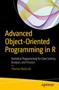
We can try to sample some lines from the prior distribution and plot them. We can, of course, plot the sample w vectors as points in the plane, but since they represent lines, we will display them as such (see Figure 4-1).
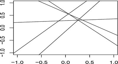
Figure 4-1. Samples from the prior of lines
prior <- prior_distribution(1)(w <- sample_weights(5, prior))## [,1] [,2]## [1,] 0.6029080 -0.84085548## [2,] 0.4721664 1.38435934## [3,] 0.6353713 -1.25549186## [4,] 0.2857736 0.07014277## [5,] -0.1381082 1.71144087plot(c(-1, 1), c(-1, 1), type = 'n',xlab = '', ylab = '')plot_lines <- function(w) {for (i in 1:nrow(w)) {abline(a = w[i, 1], b = w[i, 2])}}plot_lines(w)
When we observe data in the form of matching X and y values, we must update the w vector to reflect this, which means updating the distribution of the weights. I won’t derive the math (this is not a math textbook, after all), but if mu0 is the prior mean and S0 the prior covariance matrix, then the posterior mean and covariance matrix are computed thus:
S <- solve(S0 + b * t(X) %*% X)mu <- S %*% (solve(S0) %*% mu0 + b * t(X) %*% y)
You cannot execute the code as it is right here—it depends on variables we haven’t defined—but it is the body of the function we define shortly. It is a little bit of linear algebra that involves the prior distribution and the observed values. The parameters we haven’t seen before in these expressions are b and X. The former is the precision of the error terms—which we assume to know and represent as this hyperparameter—and the latter captures the x values. We cannot use x alone because we want to use two weights to represent lines. When we write w[1] + w[2] * x[i] for the estimate of y[i], we can think of it as the vector product of w and c(0,x[i]), which is exactly what we do. We represent all x[i] as rows c(0,x[i]) in the matrix X. So we estimate y[i] = w[1] * X[i, 1] + w[2] * X[I, 2] in this notation, or y = X %*% w.
As a fitting function, we can write it as this:
fit_posterior <- function(x, y, b, prior) {mu0 <- prior$muS0 <- prior$SX <- matrix(c(rep(1, length(x)), x), ncol = 2)S <- solve(S0 + b * t(X) %*% X)mu <- S %*% (solve(S0) %*% mu0 + b * t(X) %*% y)weight_distribution(mu = mu, S = S)}
We can try to plot some points, fit the model to these, and then plot lines sampled from the posterior. These should fall around the points now, unlike the lines sampled from the prior. The more points we use to fit the model, the tighter that lines sampled from the posterior will fall around the points (see Figure 4-2).
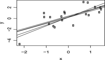
Figure 4-2. Samples of posterior lines
x <- rnorm(20)y <- 0.2 + 1.3 * x + rnorm(20)plot(x, y)posterior <- fit_posterior(x, y, 1, prior)w <- sample_weights(5, posterior)plot_lines(w)
The way we update the distribution of weights here from the prior distribution to the posterior doesn’t require that the prior distribution is the exact one we created using the variable a. Any distribution can be used as the prior, and in Bayesian statistics, it would not be unusual to update a posterior distribution as more and more data is added. We can start with the prior we just created and fit it to some data to get a posterior. Then if we get more data, we can use the first posterior as a prior for fitting more data and getting a new posterior that captures the knowledge we have gained from seeing all the data. If we have all the data from the get-go, there is no particular benefit to doing this, but in an application where data comes streaming, we can exploit this to quickly update our knowledge each time new data is available.
Since this book is not about Bayesian statistics, and since we only use Bayesian linear regression as an example of writing a new statistical model, we will not explore this further here.
Model Matrices
The X matrix we used when fitting the posterior is an example of a so-called model matrix or design matrix. Using a matrix this way, fitting a response variable, y, to some expression, here 1 + x (in a sense, we used the rows c(1, x[i])), is a general approach to fitting data. Linear models are called linear not because we fit data with a line, but because the weights, the w vector we fit, are used linearly, in the mathematical sense, in the fitted model. If we have fitted the weights to the vector w, the line we have fitted is given by X %*% w. That is, our line is the matrix product of the model matrix and the weight vector. The result is a line because X has the form we gave it, but it doesn’t have to represent a line for the model to be a linear model. We can transform the input data (here our vector x) in any way we want to before we fit the model. You might have used log-transformations before, or fitted data to a polynomial , and those would also be examples of linear models.
You can fit various kinds of transformed data using the function we wrote above if you just construct the X matrix in different ways. As long as each data point you have becomes a row in X, it doesn’t matter what you do. The same mathematics work. To fit a quadratic equation to the data instead of a line, you just have to make the ith row of X be c(1, x[i], x[i]**2), for example.
In R, you have a very powerful mechanism for constructing model matrices from formulae. Whenever you have used a formula such as y ∼ x + y to fit y to two variables, x and z, you have used this feature. The formula is translated into a model matrix, and once you have the matrix, the code that does the model fitting doesn’t need to know anything else about your data.
The function you use to translate a formula into a model matrix is called model.matrix. Even though it has a period in its name, it isn’t a generic function. It just has an unfortunate name for historical reasons.
The function will take a formula as input and produce a model matrix. It will find the values for the variables in the formula by looking in its scope, and we can use it like this:
x <- rnorm(5)y <- 1.2 + 2 * x + rnorm(5)model.matrix(y ∼ x)## (Intercept) x## 1 1 -1.1365828## 2 1 0.8548304## 3 1 -0.5783704## 4 1 0.4963615## 5 1 -0.7600579## attr(,"assign")## [1] 0 1
Relying on global variables like this is risky coding, though, so we often put our data in a data frame instead.
d <- data.frame(x, y)If we do this, we can provide a data frame to the model.matrix function and it will get the variables from there.
model.matrix(y ∼ x, data = d)## (Intercept) x## 1 1 -1.1365828## 2 1 0.8548304## 3 1 -0.5783704## 4 1 0.4963615## 5 1 -0.7600579## attr(,"assign")## [1] 0 1
If the formula uses variables that are not found in the data frame, the model.matrix will still find the missing variables in the calling scope, but this is really risky coding, so you should avoid this.
The formula determines how the model matrix is constructed. The formula y ∼ x gives us the model matrix we used above, where we have 1 to capture the intercept in the first column, and we have the x values in the second column to capture the incline of the line. We can remove the intercept using the formula y ∼ x - 1:
model.matrix(y ∼ x - 1, data = d)## x## 1 -1.1365828## 2 0.8548304## 3 -0.5783704## 4 0.4963615## 5 -0.7600579## attr(,"assign")## [1] 1
We can also add terms; for example, we can fit a quadratic formula to the data by constructing this model matrix:
model.matrix(y ∼ x + I(x**2), data = d)## (Intercept) x I(x^2)## 1 1 -1.1365828 1.2918205## 2 1 0.8548304 0.7307351## 3 1 -0.5783704 0.3345123## 4 1 0.4963615 0.2463748## 5 1 -0.7600579 0.5776881## attr(,"assign")## [1] 0 1 2
Here, we need to wrap the squared x in the function I to get R to use the actually squared values of x. Inside formulae, products are interpreted as interaction, but by wrapping x**2 in I, we make it the square of the x values explicitly.
The model matrix doesn’t include the response variable, y, so we cannot get that from it. Instead, we can use a related function, model.frame, that also gives us a column for the response.
model.frame(y ∼ x + I(x**2), data = d)## y x I(x^2)## 1 -1.4145519 -1.1365828 1.291820....## 2 0.8073317 0.8548304 0.730735....## 3 -0.2584431 -0.5783704 0.334512....## 4 0.9203396 0.4963615 0.246374....## 5 -0.5997820 -0.7600579 0.577688....
You can then extract the response variable using the function model.response, like this:
model.response(model.frame(y ∼ x + I(x**2), data = d))## 1 2 3 4## -1.4145519 0.8073317 -0.2584431 0.9203396## 5## -0.5997820
With that machinery in place, we can generalize our distributions and model fitting to work with general formulae. We can write the prior function like this:
prior_distribution <- function(formula, a, data) {n <- ncol(model.matrix(formula, data = data))mu <- rep(0, n)S <- diag(1/a, nrow = n, ncol = n)weight_distribution(mu, S)}
Ideally, a prior shouldn’t depend on any data, but the form of a model matrix does depend on the type of the data we use. Numerical data will be represented as a single column in the model matrix, but factors are handled as a binary vector for each level in a formula, so we do need to know what kind of data we are going to need. We could have added n as a parameter here and made the function independent of any data, but I chose to include a data frame as another solution. We don’t use the actual data, though; we just use it to get the number of columns in the model frame.
The function for fitting the data changes less, though. It just uses the model.matrix function to construct the model matrix instead of the explicit construction we did earlier.
fit_posterior <- function(formula, b, prior, data) {mu0 <- prior$muS0 <- prior$SX <- model.matrix(formula, data = data)S <- solve(S0 + b * t(X) %*% X)mu <- S %*% (solve(S0) %*% mu0 + b * t(X) %*% y)weight_distribution(mu = mu, S = S)}
With that in place, we can fit a line as before, but now using a formula.
d <- {x <- rnorm(5)y <- 1.2 + 2 * x + rnorm(5)data.frame(x = x, y = y)}prior <- prior_distribution(y ∼ x, 1, d)posterior <- fit_posterior(y ∼ x, 1, prior, d)posterior## $mu## [,1]## (Intercept) 1.1979166## x 0.2875647#### $S## (Intercept) x## (Intercept) 0.16935519 -0.04441203## x -0.04441203 0.73364645#### attr(,"class")## [1] "wdist"
If we, instead, want to fit a quadratic function , we do not need to change any of the functions, we can just provide a different formula.
prior <- prior_distribution(y ∼ x + I(x**2), 1, d)posterior <- fit_posterior(y ∼ x + I(x**2), 1, prior, d)posterior## $mu## [,1]## (Intercept) 1.1906733## x 0.2815418## I(x^2) 0.1185518#### $S## (Intercept) x I(x^2)## (Intercept) 0.17301554 -0.04136841 -0.05990922## x -0.04136841 0.73617725 -0.04981521## I(x^2) -0.05990922 -0.04981521 0.98053972#### attr(,"class")## [1] "wdist"
Constructing Fitted Model Objects
Now, we want to wrap fitted models in a class so we can write a constructor for them. For fitted models, it is traditional to include the formula, the data, and the function call together with the fitted model, so we will put those as attributes in the objects. The constructor could look like this:
blm <- function(formula, b, data, prior = NULL, a = NULL) {if (is.null(prior)) {if (is.null(a)) stop("Without a prior you must provide a.")prior <- prior_distribution(formula, a, data)} else {if (inherits(prior, "blm")) {prior <- prior$prior}}if (!inherits(prior, "wdist")) {stop("The provided prior does not have the expected type.")}posterior <- fit_posterior(formula, b, prior, data)structure(list(formula = formula,data = model.frame(formula, data),dist = posterior,call = match.call()),class = "blm")}
The tests at the beginning of the constructor allow us to specify the prior as either a normal distribution or a previously fitted blm object. If we get a prior distribution, we probably should also check that this prior is compatible with the actual formula , but I will let you write such a check yourself to try that out.
If we print objects fitted using the blm function, they will just be printed as a list, but we can provide our own print function by specializing the print generic function. Here, it is tradition to provide the function call used to specify the model, so that is all I will do for now.
print.blm <- function(x, ...) {print(x$call)}
We have to match the parameters of the generic function, which is why the arguments are x and…. All we do, however, is print the call attribute of the object.
Now, we can fit data and get a blm object like this:
(model <- blm(y ∼ x + I(x**2), a = 1, b = 1, data = d))## blm(formula = y ∼ x + I(x^2), b = 1, data = d, a = 1)
Coefficients and Confidence Intervals
Once we have a fitted model, we might want to get the fitted values. This is traditionally done using the generic function coef, which should simply return those. For the Bayesian linear regression model, the fitted values are whole distributions, but we can take the mean values as point estimates and return those, and so implement the coef function like this:
coef.blm <- function(object, ...) {t(object$dist$mu)}coef(model)## (Intercept) x I(x^2)## [1,] 1.190673 0.2815418 0.1185518
Here, I transform the mean matrix to get the coefficients in a form similar to what you would get with a traditional linear model, as fitted with the function lm, but other than that, the function just returns the means.
For classical frequentist models, we often also want the confidence intervals for the parameters, and the traditional way to get those is using the confint function. This function has the signature:
confint(object, parm, level = 0.95, ...)The object parameter is the fitted model, and the parm contains the parameters we want the confidence intervals for. If it is missing we should return all the model parameters, and the level parameter specifies at which confidence levels we want the intervals.
Again, for a Bayesian model, we have whole distributions and not just confidence intervals, but we can get something similar for our model by getting the quantiles from the marginal distributions for each parameter. The parameters are normally distributed, and we can get the means and standard deviations from the means and covariance matrix, respectively. After that, we can get the quantiles using the qnorm function and construct intervals like this:
confint.blm <- function(object, parm, level = 0.95, ...) {if (missing(parm)) {parm <- rownames(object$dist$mu)}means <- object$dist$mu[parm,]sds <- sqrt(diag(object$dist$S)[parm])lower_q <- qnorm(p = (1-level)/2,mean = means,sd = sds)upper_q <- qnorm(p = 1 - (1-level)/2,mean = means,sd = sds)quantiles <- cbind(lower_q, upper_q)quantile_names <- paste(100 * c((1-level)/2, 1 - (1 -level)/2),"%",sep = "")colnames(quantiles) <- quantile_namesquantiles}confint(model)## 2.5% 97.5%## (Intercept) 0.3754236 2.005923## x -1.4001225 1.963206## I(x^2) -1.8222478 2.059351
Predicting Response Variables
When it comes to predicting response variables for new data, there is a little more work to be done for the model matrix. If we don’t have the response variable when we create a model matrix, we will get an error, even though the model matrix doesn’t actually contain a column with it. We can see this if we remove the x and y variables we used when creating the data frame earlier.
rm(x) ; rm(y)We are fine if we build a model matrix from the data frame that has both x and y.
model.matrix(y ∼ x + I(x**2), data = d)## (Intercept) x I(x^2)## 1 1 -0.20409732 0.041655716## 2 1 -0.22561419 0.050901761## 3 1 0.34702845 0.120428747## 4 1 0.03236784 0.001047677## 5 1 0.41353129 0.171008128## attr(,"assign")## [1] 0 1 2
If we create a data frame that only has x values, though, we get an error.
dd <- data.frame(x = rnorm(5))model.matrix(y ∼ x + I(x**2), data = dd)## Error in eval(expr, envir, enclos): object 'y' not found
This, of course, is a problem since we are interested in predicting response variables exactly when we do not have them. This is ironic, considering that the model matrix never actually contains the response variable; nevertheless, this is how R works.
To remove the response variable from a formula, before we construct a model matrix, we need to use the function delete.response. Unfortunately, this function does not work directly on formulae, but on so-called “terms” objects. We can translate a formula into its terms using the terms function. So to remove the terms from a formula, we need the following construction:
delete.response(terms(y ∼ x))The result is a terms object, but since the terms class is a specialization of the formula class, we can use it directly with the model.matrix function to construct the model matrix.
model.matrix(delete.response(terms(y ∼ x)), data = dd)## (Intercept) x## 1 1 0.49841617## 2 1 -1.74230249## 3 1 0.97552910## 4 1 -0.02408287## 5 1 0.67568448## attr(,"assign")## [1] 0 1
Now, for actually predicting data, we traditionally use the predict generic function. This function has the following signature:
function(object, ...)Which, quite frankly, isn’t that useful. We can add to it, though, as the lm class does, so we can add a parameter newdata to it. From newdata we will construct a model matrix and make predictions for the data in this. If we just want point estimates for the new data, we can simply take the inner product of the mean weights and each row in the model matrix so we can implement the predict function like this:
predict.blm <- function(object, newdata, ...) {updated_terms <- delete.response(terms(object$formula))X <- model.matrix(updated_terms, data = newdata)predictions <- vector("numeric", length = nrow(X))for (i in seq_along(predictions)) {predictions[i] <- t(object$dist$mu) %*% X[i,]}predictions}predict(model, d)## [1] 1.138150 1.133188 1.302653 1.199910 1.327373
To check the model, we can plot the predicted values against the true response values. With the data we have used up till now, though, with only five data points, we don’t expect the predictions to be particularly good, and we don’t expect such a plot to show much, but we can try with a few more data points (see Figure 4-3).
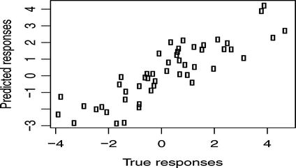
Figure 4-3. True versus predicted values
d <- {x <- rnorm(50)y <- 0.2 + 1.4 * x + rnorm(50)data.frame(x = x, y = y)}model <- blm(y ∼ x, d, a = 1, b = 1)plot(d$y, predict(model, d),xlab = "True responses",ylab = "Predicted responses")
Predicting values for the original data is so common that there is another generic function for doing this, called fitted. We can implement it like this:
fitted.blm <- function(object, ...) {predict(object, newdata = object$data, ...)}
With this function, we could then create the plot as follows:
plot(d$y, fitted(model),xlab = "True responses",ylab = "Predicted responses")
We can, of course, do more than simply predict point estimates. We have a distribution of weights, which means that the slope and intercept of a line aren’t fixed. They are, conceptually at least, drawn from a distribution. Slight changes in the slope won’t have much of an impact on how certain we are in the predictions near the main mass of the data, but data points further towards the edges of the data will have a larger uncertainty because of this. We can take the distribution into account when we make predictions to get error bars for the predictions. If X is the model matrix and S the covariance matrix for the posterior, then the variance for the ith prediction is given by:
1/b + t(X[i,]) %*% S %*% X[i,]We don’t have the precision parameter, b, stored in the fitted model object, so if we want to get error bars, we need to keep that around. So update your blm function to return this structure:
structure(list(formula = formula,data = model.frame(formula, data),dist = posterior,precision = b,call = match.call()),class = "blm")
Now, we can extend our predict function with an option that, if TRUE, returns intervals as well:
predict.blm <- function(object, newdata,intervals = FALSE,level = 0.95,...) {updated_terms <- delete.response(terms(object$formula))X <- model.matrix(updated_terms, data = newdata)predictions <- vector("numeric", length = nrow(X))for (i in seq_along(predictions)) {predictions[i] <- t(object$dist$mu) %*% X[i,]}if (!intervals) return(predictions)S <- model$dist$Sb <- model$precisionsds <- vector("numeric", length = nrow(X))for (i in seq_along(predictions)) {sds[i] <- sqrt(1/b + t(X[i,]) %*% S %*% X[i,])}lower_q <- qnorm(p = (1-level)/2,mean = predictions,sd = sds)upper_q <- qnorm(p = 1 - (1-level)/2,mean = predictions,sd = sds)intervals <- cbind(lower_q, predictions, upper_q)colnames(intervals) <- c("lower", "mean", "upper")as.data.frame(intervals)}model <- blm(y ∼ x, d, a = 1, b = 1)
With this predict function, we can plot error bars around our predictions as well, see Figure 4-4. In the figure, I also plot the x = y line. If we make accurate predictions, the point should lie on this line. Since there is some stochasticity in the data, we don’t expect to be exactly on it, but we do expect to overlap the line 95% of the time.
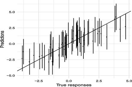
Figure 4-4. Predictions versus true values with confidence intervals
require(ggplot2)predictions <- fitted(model, intervals = TRUE)ggplot(cbind(data.frame(y = d$y), predictions),aes(x = y, y = mean)) +geom_point() +geom_errorbar(aes(ymin = lower, ymax = upper)) +geom_abline(slope = 1) +xlab("True responses") +ylab("Predictions") +theme_minimal()
There is, of course, much more we can do with a statistical model, and more generic functions we could add to it to provide a uniform interface to a class of models, but I hope this example has at least given you an impression of how representing a model as a class can be useful.