
Chapter 20
Considering Heuristics
IN THIS CHAPTER
![]() Understanding when heuristics are useful to algorithms
Understanding when heuristics are useful to algorithms
![]() Discovering how pathfinding can be difficult for a robot
Discovering how pathfinding can be difficult for a robot
![]() Getting a fast start using the best-first search
Getting a fast start using the best-first search
![]() Improving on Dijkstra’s algorithm and taking the best heuristic route using A*
Improving on Dijkstra’s algorithm and taking the best heuristic route using A*
As a concluding algorithm topic, this chapter completes the overview of heuristics started in Chapter 18 that describes heuristics as an effective means of using a local search to navigate neighboring solutions. Chapter 18 defines heuristics as educated guesses about a solution — that is, they are sets of rules of thumb pointing to the desired outcome, thus helping algorithms take the right steps toward it; however, heuristics alone can’t tell you exactly how to reach the solution.
The chapter starts by examining the different flavors of heuristics, some of which are quite popular now because of AI and robotics applications: swarm heuristics, metaheuristics; machine learning–based modeling; and heuristic routing. Next, the chapter discusses how heuristics are used by mobile robots to safely and effectively navigate known and unknown territories to accomplish their tasks. All such heuristics are based on distance, and the section “Using distance measures as heuristics” presents how two of the most common distance measures, Euclidean distance and Manhattan distance, are calculated and can help in different problem settings.
The chapter closes by demonstrating two powerful pathfinding algorithms to help robots reach their destinations safely: the best-first search algorithm and the A* (pronounced A-star) algorithm. The A* algorithm is famous because it powered Shakey the robot, as explained in the chapter. Before showing the Python code that explains how the algorithms work, the chapter also discusses how to create a maze in an effectively manner (which is an algorithm in itself) to simulate an environment with some challenges (obstacles) for the heuristic-based pathfinding algorithms to navigate.
 You don’t have to type the source code for this chapter manually. In fact, using the downloadable source is a lot easier. You can find the source for this chapter in the A4D2E; 20; Heuristic Algorithms.ipynb file of the downloadable source. See the Introduction for details on how to find this source file.
Differentiating Heuristics
The word heuristic comes from the ancient Greek heuriskein, which meant to invent or discover. Its original meaning underlines the fact that employing heuristics is a practical means of finding a solution that isn't well defined, but that is found through exploration and an intuitive grasp of the general direction to take. Heuristics rely on the lucky guess or a trial-and-error approach of trying different solutions. A heuristic algorithm, which is an algorithm powered by heuristics, solves a problem faster and more efficiently in terms of computational resources by sacrificing solution precision and completeness. These solutions are in contrast to most of the algorithms discussed so far in the book, which have certain output guarantees. When a problem becomes too complex, a heuristic algorithm can represent the only way to obtain a solution.
You have to consider that there are shades of heuristics, just as there can be shades to the truth. Heuristics touch the fringes of algorithm development today. The AI revolution builds on the algorithms presented so far in the book that order, arrange, search, and manipulate data inputs. At the top of the hierarchy are heuristic algorithms that power optimization, as well as searches that determine how machines learn from data and become capable of solving problems autonomously from direct intervention.
Heuristics aren’t silver bullets; no solution solves every problem. Heuristic algorithms have serious drawbacks, and you need to know when to use them. In addition, heuristics can lead to wrong conclusions for both computers and humans.
In fact, for humans, everyday heuristics that save time can often prove wrong, such as when evaluating a person or situation at first glance in a prejudiced manner. Even more reasoned rules of conduct taken from experience obtain the right solution only under certain circumstances. For instance, consider the habit of hitting electric appliances when they don’t work. If the problem is a loose connection, hitting the appliance may prove beneficial by reestablishing the electric connection, but you can’t make hitting appliances a general heuristic because in other cases, that “solution” may prove ineffective or even cause serious damage to the appliance.
Considering the goals of heuristics
Heuristics can speed the long, exhaustive searches performed by other solutions, especially with NP-hard problems that require an exponential number of attempts based on the number of their inputs. For example, consider the traveling salesman problem or variants of the SAT problem (2-SAT appears in Chapter 18), such as the MAX-3SAT (see https://people.maths.bris.ac.uk/~csxam/bccs/approx.pdf for additional details). Heuristics determine the search direction using an estimation, which eliminates a large number of the combinations it would have to test otherwise.
Because a heuristic is an estimate or a guess, it can lead the algorithm that relies on it to a wrong conclusion, which could be an inexact solution or just a suboptimal solution. A suboptimal solution is a solution that works, but is not the best possible. For example, in a numerical estimation, a heuristic might provide a solution that is a few numbers off the correct answer. This suboptimal solution might be acceptable for many situations, but some situations require an exact solution. Other problems often associated with heuristics are the impossibility of finding all the best solutions as well as the variability of time and computations required to reach a solution. A heuristic provides a perfect match when working with algorithms that would otherwise incur a high cost when interacting with other algorithmic techniques. For instance, you can’t solve certain problems without heuristics because of the poor quality and overwhelming number of data inputs. The traveling salesman problem (TSP) is one of these: If you have to tour a large number of cities, you can’t use any exact method. TSP and other problems exclude any exact solution. AI applications fall into this category because many AI problems, such as recognizing spoken words or the content of an image, aren’t solvable in an exact sequence of steps and rules.
Going from genetic to AI
The Chapter 18 local search discussion presents heuristics such as simulated annealing and Tabu Search. You use these heuristics to help with hill-climbing optimization (an optimization that helps by not getting stuck with solutions that are less than ideal). Apart from these, the family of heuristics comprises many different applications, among which are the following:
- Swarm intelligence: A set of heuristics based on the study of the behavior of insect swarms (such as bees, ants, or fireflies) or particles. The method uses multiple attempts to find a solution using agents that interact cooperatively between themselves and the problem setting. An agent is an independent computational unit, such as when running several independent instances of the same algorithm, with each one working on a different piece of the problem. Professor Marco Dorigo, one of the top experts and contributors on the study of swarm intelligence algorithms, provides more information on this topic at
https://scholar.google.com/citations?user=PwYT6EMAAAAJ(which contains a listing of his various works). - Metaheuristics: Heuristics that help you determine (or even generate) the right heuristic for your problem. Among metaheuristics, the most widely known are genetic algorithms, inspired by natural evolution. Genetic algorithms start with a pool of possible problem solutions and then generate new solutions using mutation (they add or remove something in the solution) and cross-over (they mix parts of different solutions when a solution is divisible). For instance, in the n-queens problem (Chapter 18), you see that you can split a chessboard vertically into parts because the queens don’t move horizontally as part of the problem solution, making it a problem suitable for cross-over. When the pool is large enough, genetic algorithms select the surviving solutions by ruling out those that don’t work or lack promise. The selected pool then undergoes another iteration of mutation, cross-over, and selection. After enough time and iterations, genetic algorithms can find solutions that perform better and are completely different from the initial ones.
- Machine learning: Approaches such as neuro-fuzzy systems, support vector machines, and neural networks are the foundation of how a computer learns to estimate and classify from training examples that are provided as part of sets of data. Similarly to how a child learns by experience, machine learning algorithms determine how to deliver the most plausible answer without using precise rules and detailed rules of conduct. (See Machine Learning For Dummies, 2nd Edition, by John Paul Mueller and Luca Massaron [Wiley], for details on how machine learning works.)
- Heuristic routing: A set of heuristics that helps robots (but is also found in network telecommunications and transportation logistics) to choose the best path to avoid obstacles when moving around.
Routing Robots Using Heuristics
Guiding a robot in an unknown environment means avoiding obstacles and finding a way to reach a specific target. It’s both a fundamental and challenging task in artificial intelligence. Robots can rely on different sensors such as laser rangefinder, lidar (devices that allow you to determine the distance to an object by means of a laser ray), or sonar arrays (devices that use sounds to see their environment) to navigate their surroundings. Yet, the sophistication of the hardware used to equip robots doesn’t matter; robots still need proper algorithms to:
- Find the shortest path to a destination (or at least a reasonably short one)
- Avoid obstacles on the way
- Perform custom behaviors such as minimizing turning or braking
A pathfinding (also called path planning or simply pathing) algorithm helps a robot start in one location and reach a goal using the shortest path between the two, anticipating and avoiding obstacles along the way. (It isn’t enough to react after hitting a wall.) Pathfinding is also useful when moving any other device to a target in space, even a virtual one, such as in a video game or the pages on websites.
Routing autonomously is a key capability of self-driving cars (SDC), which are vehicles that can sense the road environment and drive to the destination without any human intervention. (You still need to tell the car where to go; it can’t read minds.) This recent article from Automotive World Magazine offers a good overview about the developments and expectations for self-driving cars: https://www.automotiveworld.com/articles/the-future-of-driving-what-to-expect-in-2021/.
Scouting in unknown territories
Pathfinding algorithms accomplish all the previously discussed tasks to achieve shortest routing, obstacle avoidance, and other desired behaviors. Algorithms work by using basic schematic maps of their surroundings. These maps are of two kinds:
- Topological maps: Simplified diagrams that remove every unnecessary detail. The maps retain key landmarks, correct directions, and some scale proportions for distances. Real-life examples of topological maps include subway maps of Tokyo (
https://www.tokyometro.jp/en/subwaymap/) and London (https://tfl.gov.uk/maps/track/tube). - Occupancy grid maps: These maps divide the surroundings into small, empty squares or hexagons, filling them in when the robot’s sensors find an obstacle on the spot they represent. You can see an example of such a map at the Czech Technical University in Prague:
http://cmp.felk.cvut.cz/cmp/demos/Omni/mobil/. In addition, check out the videos showing how a robot builds and visualizes such a map athttps://www.youtube.com/watch?v=zjl7NmutMIcandhttps://www.youtube.com/watch?v=RhPlzIyTT58.
You can visualize both topological and occupancy grid maps as graphic diagrams. However, they’re best understood by algorithms when rendered into an appropriate data structure. The best data structure for this purpose is the graph because vertexes can easily represent squares, hexagons, landmarks, and waypoints. Edges can connect vertexes in the same way that roads, passages, and paths do.
Your GPS navigation device operates using graphs. Underlying the continuous, detailed, colorful map that the device displays on screen, road maps are elaborated behind the scenes as sets of vertexes and edges traversed by algorithms helping you find the way while avoiding traffic jams.
Representing the robot’s territory as a graph re-introduces problems discussed in Chapter 9, which examines how to travel from one vertex to another using the shortest path. The shortest path can be the path that touches the fewest vertexes or the path that costs less (given the sum of the cost of the crossed edge weights, which may represent the length of the edge or some other cost). As when driving your car, you choose a route based not only on the distance driven to reach your destination but also on traffic (roads crowded with traffic or blocked by traffic jams), road conditions, and speed limits that may influence the quality of your journey.
When finding the shortest path to a destination in a graph, the simplest and most basic algorithms in graph theory are depth-first search and Dijkstra’s algorithm (described in Chapter 9). Depth-first search explores the graph by going as far as possible from the start and then retracing its steps to explore other paths until it finds the destination. Dijkstra’s algorithm explores the graph in a smart and greedy way, considering only the shortest paths. Despite their simplicity, both algorithms are extremely effective when evaluating a simple graph, as in a bird’s- eye view, with complete knowledge of the directions you must take to reach the destination and little cost in evaluating the various possible paths.
The situation with a robot is slightly different because it can’t perceive all the possible paths at one time, being limited in both visibility and range of sight (obstacles may hide the path or the target may be too far). A robot discovers its environment as it moves and, at best, can assess the distance and direction of its final destination. It’s like solving a maze, though not as when playing in a puzzle maze but more akin to immersion in a hedge maze, where you can feel the direction you are taking or you can spot the destination in the distance.
 Hedge mazes are found everywhere in the world. Some of the most famous were built in Europe from the mid-16th century to eighteenth century. In a hedge maze, you can’t see where you’re going because the hedges are too high. You can perceive direction (if you can see the sun) and even spot the target (see
 https://www.venetoinside.com/hidden-treasures/post/maze-of-villa-pisani-in-stra-venice/ as an example). There are also famous hedge mazes in films such as The Shining by Stanley Kubrick and in Harry Potter and the Goblet of Fire.
Using distance measures as heuristics
When you can’t solve real-life problems in a precise algorithmic way because their input is confused, missing, or unstable, using heuristics can help. When performing path finding using coordinates in a Cartesian plane (flat maps that rely on a set of horizontal and vertical coordinates), two simple measures can provide the distances between two points in that plane: the Euclidean distance and the Manhattan distance.
People commonly use the Euclidean distance because it derives from the Pythagorean Theorem on triangles and represents the shortest distance between two points. If you want to know the distance in line of sight between two points in a plane, say, A and B, and you know their coordinates, you can pretend they’re the extremes of the hypotenuse (the longest side in a right triangle). As depicted in Figure 20-1, you calculate distance based on the length of the other two sides by creating a third point, C, whose horizontal coordinate is derived from B and whose vertical coordinate is from A.

FIGURE 20-1: A and B are points on a map’s coordinates.
This process translates into taking the difference between the horizontal and vertical coordinates of your two points, squaring both the differences (so that they both become positive), sum them, and finally taking the square root of the result. In this example, going from A to B uses coordinates of (1,2) and (3,3):
sqrt((1-3)2 + (2-3)2) = sqrt(22+12) = sqrt(5) = 2.236
You actually can’t measure distances on the Earth’s surface exactly using the Euclidean distance because its surface isn’t flat but is instead near spherical. As the distances between points you measure on the Earth’s surface increase, the Euclidean distance underestimation will also increase. Measures that are more appropriate when long distances are involved are the haversine distance based on latitude and longitude coordinates (see https://www.igismap.com/haversine-formula-calculate-geographic-distance-earth/) or the more exact Vincenty distance (see https://metacpan.org/pod/GIS::Distance::Vincenty).
The Manhattan distance works differently. You begin by summing the lengths of the sides b and c, which equates summing the absolute value of the differences between the horizontal and vertical coordinates of the points A and B.
|(1-3)| + |(2-3)| = 2 + 1 = 3
The Euclidean distance marks the shortest route, and the Manhattan distance provides the longest yet most plausible route if you expect obstacles when taking a direct route. In fact, the movement represents the trajectory of a taxi in Manhattan (hence the name), moving along a city block to reach its destination (taking the short route through buildings would never work). Other names for this approach are the city block distance or the taxicab distance. Consequently, if you have to move from A to B but you don’t know whether you’ll find obstacles between them, taking a detour through point C is a good heuristic because that’s the distance you expect at worst.
Explaining Path Finding Algorithms
This last part of the chapter concentrates on explaining two algorithms, best-first search and A* (read as A-star), both based on heuristics. The following sections demonstrate that both of these algorithms provide a fast solution to a maze problem representing a topological or occupancy grid map that’s represented as a graph. Both algorithms are widely used in robotics and video gaming.
Creating a maze
A topological or occupancy grid map resembles a hedge maze, as mentioned previously, especially if obstacles exist between the start and the end of the route. There are specialized algorithms for both creating and processing mazes, most notably the Wall Follower (known since antiquity: You place your hand on a wall and never pull it away until you get out of the maze) or the Pledge algorithm. (Read more about the seven maze classifications at http://www.astrolog.org/labyrnth/algrithm.htm.) However, pathfinding is fundamentally different from maze solving because in pathfinding, you know where the target should be, whereas maze-solving algorithms try to solve the problem in complete ignorance of where the exit is.
Consequently, the procedure for simulating a maze of obstacles that a robot has to navigate takes a different and simpler approach. Instead of creating a riddle of obstacles, you create a graph of vertexes arranged in a grid (resembling a map) and randomly remove connections to simulate the presence of obstacles. The graph is undirected (you can traverse each edge in both directions) and weighted because it takes time to move from one vertex to another. In particular, it takes longer to move diagonally than t upward/downward or left/right.
The first step is to import the necessary Python packages. The code defines the Euclidean and the Manhattan distance functions next. (You can find this code in the A4D2E; 20; Heuristic Algorithms.ipynb downloadable source code file; see the Introduction for details.)
import string
import networkx as nx
import matplotlib.pyplot as plt
import random

def euclidean_dist(a, b, coord):
    (x1, y1) = coord[a]
    (x2, y2) = coord[b]
    return ((x1 - x2)**2 + (y1 - y2)**2)**0.5

def manhattan_dist(a, b, coord):
    (x1, y1) = coord[a]
    (x2, y2) = coord[b]
    return abs(x1 - x2) + abs(y1 - y2)

def non_informative(a,b):
    return 0

def ravel(listsoflists):
    return [item for elem in listsoflists for item in elem]
The next step creates a function to generate random mazes. It's based on an integer number seed of your choice that allows you to recreate the same maze every time you provide the same number. Otherwise, maze generation is completely random. There is also a general function, node_neighbors()
def node_neighbors(graph, node):
    return [exit for _,
            exit in graph.edges(node) if exit!=node]

def create_maze(seed=2, drawing=True):
    random.seed(seed)
    letters = [l for l in string.ascii_uppercase[:25]]
    checkboard = [letters[i:i+5]
                  for i in range(0, len(letters), 5)]
    Graph = nx.Graph()
    for j, node in enumerate(letters):
        Graph.add_nodes_from(node)
        x, y = j // 5, j % 5
        x_min = max(0, x-1)
        x_max = min(4, x+1)+1
        y_min = max(0, y-1)
        y_max = min(4, y+1)+1
        adjacent_nodes = ravel(
            [row[y_min:y_max]
             for row in checkboard[x_min:x_max]])
        exits = random.sample(adjacent_nodes,
                              k=random.randint(1, 4))
        for exit in exits:
            if exit not in node_neighbors(Graph, node):
                Graph.add_edge(node, exit)
    spacing = [0.0, 0.2, 0.4, 0.6, 0.8]
    coordinates = [[x, y] for x in spacing
                   for y in spacing]
    position  = {l:c for l,c in zip(letters, coordinates)}

    for node in Graph.nodes:
        for exit in node_neighbors(Graph, node):
            length = int(round(
                    euclidean_dist(
                        node, exit, position)*10,0))
            Graph.add_edge(node,exit,weight=length)

    if drawing:
        draw_params = {'with_labels':True,
                       'node_color':'skyblue',
                       'node_size':700, 'width':2,
                       'font_size':14}
        nx.draw(Graph, position, **draw_params)
        labels = nx.get_edge_attributes(Graph,'weight')
        nx.draw_networkx_edge_labels(Graph, position,
                                     edge_labels=labels)
        plt.show()

    return Graph, position
The functions return a NetworkX graph (Graph), a favorite data structure for representing graphs, which contains 25 vertexes (or nodes, if you prefer) and a Cartesian map of points (position). The vertexes are placed on a 5-x-5 grid, as shown in Figure 20-2. The output also applies distance functions and calculates the position of vertexes.
graph, coordinates = create_maze(seed=7)
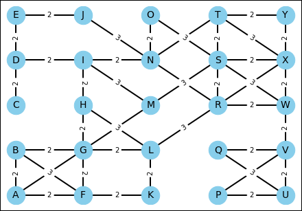
FIGURE 20-2: A maze representing a topological map with obstacles.
In the maze generated by a seed value of 7, every vertex connects with the others. Because the generation process is random, some maps may contain disconnected vertexes, which precludes going between the disconnected vertexes. To see how this works, try a seed value of 6. This actually happens in reality; for example, sometimes a robot can't reach a particular destination because it’s surrounded by obstacles.
Looking for a quick best-first route
The depth-first search algorithm explores the graph by moving from vertex to vertex and adding directions to a stack data structure. When it’s time to move, the algorithm moves to the first direction found on the stack. It’s like moving through a maze of rooms by taking the first exit you see. Most probably, you arrive at a dead end, which isn’t your destination. You then retrace your steps to the previously visited rooms to see whether you encounter another exit, but it takes a long time when you’re far from your target.
Heuristics can greatly help with the repetition created by a depth-first search strategy. Using heuristics can tell you whether you’re getting nearer or farther from your target. This combination is called the best-first search algorithm (BFS). In this case, the best in the name hints at the fact that, as you explore the graph, you don’t take the first edge in sight. Rather you evaluate which edge to take based on the one that should take you closer to your desired outcome based on the heuristic. This behavior resembles greedy optimization (the best first), and some people also call this algorithm greedy best-first search. BFS will probably miss the target at first, but because of heuristics, it won’t end up far from target and will retrace less than it would if using depth-first search alone.
You use the BFS algorithm principally in web crawlers that look for certain information on the web. In fact, BFS allows a software agent to move in a mostly unknown graph, using heuristics to detect how closely the content of the next page resembles the initial one (to explore for better content). The algorithm is also widely used in video games, helping characters controlled by the computer move in search of enemies and bounties, thereby resembling a greedy, target-oriented behavior.
Demonstrating BFS in Python using the previously built maze illustrates how a robot can move in a space by seeing it as a graph. The following code shows some general functions, which are also used for the next algorithm in this section. The graph_weight() function determines the cost of going from one vertex to another. Weight represents distance or time.
def graph_weight(graph, a, b):
    return graph.edges[(a, b)]['weight']
The path-planning algorithm simulates robot movement in a graph. When it finds a solution, the plan translates into movement. Therefore, path-planning algorithms provide an output telling you how to best move from one vertex to another; you still need a function to translate the information and determine the route to take and calculate trip length. The functions reconstruct_path() and compute_path() provide the plan in terms of steps and expected cost when given the result from the path-planning algorithm.
def reconstruct_path(connections, start, goal):
    if goal in connections:
        current = goal
        path = [current]
        while current != start:
            current = connections[current]
            path.append(current)
        return path[::-1]

def compute_path_dist(path, graph):
    if path:
        run = 0
        for step in range(len(path)-1):
            A = path[step]
            B = path[step+1]
            run += graph_weight(graph, A, B)
        return run
    else:
        return 0
Having prepared all the basic functions, the example creates a maze using a seed value of 30. This maze presents a few main routes going from vertex A to vertex Y because there are some obstacles in the middle of the map (as shown in Figure 20-3). There is also a dead end on the way (vertex I).
graph, coordinates = create_maze(seed=30)
start = 'A'
goal  = 'Y'
scoring = manhattan_dist
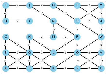
FIGURE 20-3: An intricate maze to be solved by heuristics.
The BFS implementation is a bit more complex than the depth-first search code found in Chapter 9. It uses two lists: one to hold the never-visited vertexes (called open_list), and another to hold the visited ones (closed_list). The open_list list acts as a priority queue, one in which a priority determines the first element to extract. In this case, the heuristic provides the priority, thus the priority queue provides a direction that's closer to the target. The Manhattan distance heuristic works best because of the obstacles obstructing the way to the destination:
# Best-first search
path = {}
open_list = set(graph.nodes())
closed_list = {start: manhattan_dist(start, goal,
                                     coordinates)}

while open_list:

    candidates = open_list&closed_list.keys()
    if len(candidates)==0:
        print ("Cannot find a way to the goal %s" % goal)
        break
    frontier = [(closed_list[node],
                 node) for node in candidates]
    score, min_node =sorted(frontier)[0]

    if min_node==goal:
        print ("Arrived at final vertex %s" % goal)
        print ('Unvisited vertices: %i' % (len(
                    open_list)-1))
        break
    else:
        print("Processing vertex %s, " % min_node, end="")

    open_list = open_list.difference(min_node)
    neighbors = node_neighbors(graph, min_node)
    to_be_visited = list(neighbors-closed_list.keys())

    if len(to_be_visited) == 0:
        print ("found no exit, retracing to %s"
               % path[min_node])
    else:
        print ("discovered %s" % str(to_be_visited))

    for node in neighbors:
        if node not in closed_list:
            closed_list[node] = scoring(node, goal,
                                        coordinates)
            path[node] = min_node

print ('
Best path is:', reconstruct_path(
        path, start, goal))
print ('Length of path: %i' % compute_path_dist(
        reconstruct_path(path, start, goal), graph))
The verbose output from the example tells you how the algorithm works:
Processing vertex A, discovered ['F', 'B', 'G']
Processing vertex G, discovered ['H', 'C', 'L', 'K']
Processing vertex H, discovered ['M']
Processing vertex M, discovered ['R', 'N']
Processing vertex N, discovered ['J']
Processing vertex J, discovered ['E', 'O']
Processing vertex O, discovered ['S', 'T']
Processing vertex T, discovered ['Y', 'X']
Arrived at final vertex Y
Unvisited vertices: 16

Best path is: ['A', 'G', 'H', 'M', 'N', 'J', 'O', 'T', 'Y']
Length of path: 18
BFS keeps moving until it runs out of vertexes to explore. When it exhausts the vertexes without reaching the target, the code tells you that it can’t reach the target and the robot won’t budge. When the code does find the destination, it stops processing vertexes, even if open_list still contains vertexes, which saves time.
Finding a dead end, such as ending up in vertex I, means looking for a previously unused route. The best alternative immediately pops up thanks to the priority queue, and the algorithm takes it. In this example, BFS efficiently ignores 16 vertexes and takes the upward route in the map, completing its journey from A to Y in 18 steps.
You can test other mazes by setting a different seed number and comparing the BFS results with the A* algorithm described in the next section. You'll find that sometimes BFS is both fast and accurate in choosing the best way, and sometimes it’s not. If you need a robot that searches quickly, BFS is the best choice.
Going heuristically around by A*
The A* algorithm speedily produces best shortest paths in a graph by combining the Dijikstra greedy search discussed in Chapter 9 with an early stop (the algorithm stops when it reaches its destination vertex) and a heuristic estimate (usually based on the Manhattan distance) that hints at the graph area to explore first. A* was developed at the Artificial Intelligence Center of Stanford Research Institute (now called SRI International) in 1968 as part of the Shakey the robot project. Shakey was the first mobile robot to autonomously decide how to go somewhere, although it was limited to wandering around a few rooms in the labs. (If you watch the video at https://www.youtube.com/watch?v=qXdn6ynwpiI, you see that it’s the person filming who’s shaky, not the robot. But, as always, it’s easier to blame the robot.) Shakey was a milestone robotic implementation that demonstrated how it was technologically possible to build a mobile robot operating without human supervision at the end of the 1960s.
To render Shakey fully autonomous, its developers came up with the A* algorithm, the Hough transform (an image-processing transformation to detect the edges of an object), and the visibility graph method (a way to represent a path as a graph). The article at http://www.ai.sri.com/shakey/ describes Shakey in more detail and even shows it in action. The A* algorithm is currently the best available algorithm when you’re looking for the shortest route in a graph and you must deal with partial information and expectations (as captured by the heuristic function guiding the search). A* is able to
- Find the shortest path solution every time: The algorithm can do this if such a path exists and if A* is properly informed by the heuristic estimate. A* is powered by the Dijkstra algorithm, which guarantees always finding the best solution.
- Find the solution faster than any other algorithm: A* can do this if given access to a fair heuristic — one that provides the right directions to reach the target proximity in a similar, though even smarter, way as BFS.
- Computes weights when traversing edges: Weights account for the cost of moving in a certain direction. For example, turning may take longer than going straight, as in the case of Shakey the robot.
A proper, fair, admissible heuristic provides useful information to A* about the distance to the target by never overestimating the cost of reaching it. Moreover, A* makes greater use of its heuristic than BFS, therefore the heuristic must perform calculations quickly or the overall processing time will be too long.
The Python implementation in this example uses the same code and data structures used for BFS, but there are differences between them. The main differences are that as the algorithm proceeds, it updates the cost of reaching from the start vertex to each of the explored vertexes. In addition, when it decides on a route, A* considers the shortest path from the start to the target, passing by the current vertex, because it sums the estimate from the heuristic with the cost of the path computed to the current vertex. This process allows the algorithm to perform more computations than BFS when the heuristic is a proper estimate and to determine the best path possible.
Finding the shortest path possible in cost terms is the core Dijkstra algorithm function. A* is simply a Dijkstra algorithm in which the cost of reaching a vertex is enhanced by the heuristic of the expected distance to the target. Chapter 9 describes the Dijkstra algorithm in detail. Revisiting the Chapter 9 discussion will help you better understand how A* operates in leveraging heuristics.
# A*
open_list = set(graph.nodes())
closed_list = {start: manhattan_dist(
        start, goal, coordinates)}
visited = {start: 0}
path = {}

while open_list:

    candidates = open_list&closed_list.keys()
    if len(candidates)==0:
        print ("Cannot find a way to the goal %s" % goal)
        break
    frontier = [(closed_list[node],
                 node) for node in candidates]
    score, min_node =sorted(frontier)[0]

    if min_node==goal:
        print ("Arrived at final vertex %s" % goal)
        print ('Unvisited vertices: %i' % (len(
                open_list)-1))
        break
    else:
        print("Processing vertex %s, " % min_node, end="")

    open_list = open_list.difference(min_node)
    current_weight = visited[min_node]
    neighbors = node_neighbors(graph, min_node)
    to_be_visited = list(neighbors-visited.keys())
    for node in neighbors:
        new_weight = current_weight + graph_weight(
                     graph, min_node, node)
        if node not in visited or
        new_weight < visited[node]:
            visited[node] = new_weight
            closed_list[node] = manhattan_dist(node, goal,
                        coordinates) + new_weight
            path[node] = min_node

    if to_be_visited:
        print ("discovered %s" % to_be_visited)
    else:
        print ("getting back to open list")

print ('
Best path is:', reconstruct_path(
        path, start, goal))
print ('Length of path: %i' % compute_path_dist(
        reconstruct_path(path, start, goal), graph))
When the A* has completed analyzing the maze, it outputs a best path that’s shorter than the BFS solution:
Processing vertex A, discovered ['F', 'B', 'G']
Processing vertex B, discovered ['C']
Processing vertex F, discovered ['L', 'K']
Processing vertex G, discovered ['H']
Processing vertex C, getting back to open list
Processing vertex K, discovered ['Q', 'P']
Processing vertex H, discovered ['M']
Processing vertex L, discovered ['R']
Processing vertex P, discovered ['U', 'V']
Processing vertex M, discovered ['N']
Processing vertex Q, discovered ['W']
Processing vertex R, discovered ['S']
Processing vertex U, getting back to open list
Processing vertex N, discovered ['J']
Processing vertex V, getting back to open list
Processing vertex S, discovered ['Y', 'X', 'O']
Processing vertex W, getting back to open list
Processing vertex X, discovered ['T']
Processing vertex J, discovered ['E']
Arrived at final vertex Y
Unvisited vertices: 5

Best path is: ['A', 'F', 'L', 'R', 'S', 'Y']
Length of path: 13
This solution comes at a cost: A* explores almost all the present vertexes, leaving just five vertexes unconsidered. As with Dijkstra, its worst running time is O(v2), where v is the number of vertexes in the graph; or O(e + v*log(v)), where e is the number of edges, when using min-priority queues, an efficient data structure when you need to obtain the minimum value for a long list. The A* algorithm is not different in its worst running time than Dijkstra’s, though on average, it performs better on large graphs because it first finds the target vertex when correctly guided by the heuristic measurement (in the case of a routing robot, the Manhattan distance).