2
TAKING STOCK: A RIGOROUS MODELLING OF ANIMAL SPIRITS IN MACROECONOMICS
Reiner Franke
University of Kiel (GER)
Frank Westerhoff
University of Bamberg (GER)
1. Introduction
A key issue in which heterodox macroeconomic theory differs from the orthodoxy is the notion of expectations, where it determinedly abjures the rational expectations hypothesis. Instead, to emphasize its view of a constantly changing world with its fundamental uncertainty, heterodox economists frequently refer to the famous idea of the ‘animal spirits’. This is a useful keyword that poses no particular problems in general conceptual discussions. However, given the enigma surrounding the expression, what can it mean when it comes to rigorous formal modelling? More often than not, authors garland their model with this word, even if there may be only loose connections to it. The present survey focusses on heterodox approaches that take the notion of the ‘animal spirits’ more seriously and, seeking to learn more about its economic significance, attempt to design dynamic models that are able to definitively capture some of its crucial aspects.1
The background of the term as it is commonly referred to is Chapter 12 of Keynes' General Theory, where he discusses another elementary ‘characteristic of human nature’, namely, ‘that a large proportion of our positive activities depend on spontaneous optimism rather than on a mathematical expectation’ (Keynes, 1936, p. 161). Although the chapter is titled ‘The state of long-term expectation’, Keynes makes it clear that he is concerned with ‘the state of psychological expectation’ (p. 147).2
It is important to note that this state does not arise out of the blue from whims and moods; it is not an imperfection or plain ignorance of human decision makers. Ultimately, it is due to the problem that decisions resulting in consequences that reach far into the future are not only complex, but also fraught with irreducible uncertainty. ‘About these matters’, Keynes wrote elsewhere to clarify the basic issues of the General Theory, ‘there is no scientific basis on which to form any calculable probability whatever’ (Keynes, 1937, p. 114). Needless to say, this facet of Keynes' work is completely ignored by the ‘New-Keynesian’ mainstream.
To cope with uncertainty that cannot be reduced to a mathematical risk calculus, enabling us nevertheless ‘to behave in a manner which saves our faces as rational economic men’, Keynes (1937) refers to ‘a variety of techniques’, or ‘principles’, which are worth quoting in full.
- (1) We assume that the present is a much more serviceable guide to the future than a candid examination of past experience would show it to have been hitherto. In other words, we largely ignore the prospect of future changes about the actual character of which we know nothing'.
- (2) We assume that the existing state of opinion as expressed in prices and the character of existing output is based on a correct summing up of future prospects, so that we can accept it as such unless and until something new and relevant comes into the picture.
- (3) Knowing that our own individual judgment is worthless, we endeavor to fall back on the judgment of the rest of the world which is perhaps better informed. That is, we endeavor to conform with the behavior of the majority or the average. The psychology of a society of individuals each of whom is endeavoring to copy the others leads to what we may strictly term a conventional judgment. (p. 114; his emphasis)3
The third point is reminiscent of what is currently referred to in science and the media as herding. As it runs throughout Chapter 12 of the General Theory, decision makers are not very concerned with what an investment might really be worth; rather, under the influence of mass psychology, they devote their intelligences ‘to anticipating what average opinion expects the average opinion to be’, a judgement of ‘the third degree’ (Keynes, 1936, p. 156). Note that it is rational in such an environment ‘to fall back on what is, in truth, a convention’ (Keynes, 1936, p. 152; Keynes' emphasis). Going with the market rather than trying to follow one's own better instincts is rational for ‘persons who have no special knowledge of the circumstances’ (p. 153) as well as for expert professionals.
If the general phenomenon of forecasting the psychology of the market is taken for granted, then it is easily conceivable how waves of optimistic or pessimistic sentiment are generated by means of a self-exciting, possibly accelerating mechanism. Hence, any modelling of animal spirits will have to attempt to incorporate a positive feedback effect of this kind.
The second point in the citation refers to more ‘objective’ factors such as prices or output (or, it may be added, composite variables derived from them). According to the first point, it is the current values that are most relevant for the decision maker. According to the second point, this is justified by his or her assumption that these values are the result of a correct anticipation of the future by the other, presumably smarter and, in their entirety, better informed market participants.
If one likes, it could be said that the average opinion also plays a role here, only in a more indirect way. In any case, insofar as agents believe in the objective factors mentioned above as fundamental information, they will have a bearing on the decision-making process. Regarding modelling, current output, prices and the like could therefore be treated in the traditional way as input in a behavioural function. In the present context, however, these ordinary mechanisms will have to be reconciled with the direct effects of the average opinion. It is then a straightforward idea that the ‘fundamentals’ may reinforce or keep a curb on the ‘conventional’ dynamics.
In the light of this discussion, formal modelling does not seem to be too big a problem: set up a positive feedback loop for a variable representing the ‘average opinion’ and combine it with ordinary behavioural functions. In principle, this can be, and has been, specified in various ways. The downside of this creativity is that it makes it hard to compare the merits and demerits of different models, even if one is under the impression that they invoke similar ideas and effects. Before progressing too far to concrete modelling, it is therefore useful to develop building blocks, or to have reference to existing blocks, which can serve as a canonical schema.
Indeed, modelling what may be interpreted as animal spirits is no longer virgin territory. Promising work has been performed over the last 10 years that can be subdivided into three categories (further details later). Before discussing them one by one, we set up a unifying frame of reference which makes it easier to site a model. As a result, it will also be evident that the models in the literature have more in common than it may seem at first sight. In particular, it is not by chance that they have similar dynamic properties.
The work we focus on is all the more appealing since it provides a micro-foundation of macroeconomic behaviour, albeit, of course, a rather stylized one. At the outset, the literature refers to a large population of agents who, for simplicity, face a binary decision. For example, they may choose between optimism and pessimism, or between extrapolative and static expectations about prices or demand. Individual agents do this with certain probabilities and then take a decision. The central point is that probabilities endogenously change in the course of time. They adjust upward or downward in reaction to agents' observations, which may include output, prices as well as the aforementioned ‘average opinion’. As a consequence, agents switch between two attitudes or two strategies. Their decisions vary correspondingly, as does the macroeconomic outcome resulting from them.
By the law of large numbers, this can all be cast in terms of aggregate variables, where one such variable represents the current population mix. The relationships between them form an ordinary and well-defined macrodynamic system specified in discrete or continuous time, as the case may be. The animal spirits and their variations, or that of the average opinion, play a crucial role as the dynamic properties are basically determined by the switching mechanism.
Owing to the increasing and indiscriminate use of the emotive term ‘animal spirits’, causing it to become an empty phrase, we will in the course of our presentation distinguish between a weak and a strong form of animal spirits in macrodynamics. We will refer to a weak form if a model is able to generate waves of, say, an optimistic and pessimistic attitude, or waves of applying a forecast rule 1 as opposed to a forecast rule 2. A prominent argument for this behaviour is that the first rule has proven to be more successful in the recent past. A strong form of animal spirits is said to exist if agents also rush towards an attitude, strategy, or so on, simply because it is being applied at the time by the majority of agents. In other words, this will be the case if there is a component of herding in the dynamics because individual agents believe that the majority will probably be better informed and smarter than they themselves. To give a first overview, the weak form of animal spirits will typically be found in macro-models employing what is known as the discrete choice approach (DCA), whereas models in which we identify the strong form typically choose the so-called transition probability approach (TPA). However, this division has mainly historical rather than logical reasons.
The remainder of this survey is organized as follows. The next section introduces the two approaches just mentioned. It also points out that they are more closely related than it may appear at first sight and then sets up an abstract two-dimensional model that allows us to study the dynamic effects that they possibly produce. In this way, it can be demonstrated that it is the two approaches themselves and their inherent non-linearities that, with little additional effort, are conducive to the persistent cyclical behaviour emphasized by most of the literature.
Section 3 is concerned with a class of models that are concerned with heterogeneous rule-of-thumb expectations within the New-Keynesian three-equation model (but without its rational expectations). This work evaluates the fitness of the two expectation rules by means of the discrete choice probabilities. It is also noteworthy because orthodox economists have shown an interest in it and given it attention. Section 4 discusses models with an explicit role for herding, which, as stated, is a field for the TPA (and where we will also reason about the distinction between animal spirits in a weak and strong form).4
While the modelling outlined so far is conceptually attractive for capturing a sentiment dynamics, it would also be desirable to have some empirical support for it. Section 5 is devoted to this issue. Besides some references to laboratory experiments, it covers work that investigates whether the dynamics of certain business survey indices can be explained by a suitable application of (mainly) the TPA. On the other hand, it presents work that takes a model from Section 3 or 4 and seeks to estimate it in its entirety. Here, the sentiment variable is treated as unobservable and only its implications for the dynamics of the other, observable macro-variables are taken into account. Section 6 concludes.
2. The General Framework
The models we shall survey are concerned with a large population of agents who have to choose between two alternatives. In principle, their options can be almost anything: strategies, rules of thumb to form expectations, diffuse beliefs. In fact, this is a first feature in which the models may differ. For concreteness, let us refer in the following general introduction to two attitudes that agents may entertain and call them optimism and pessimism, identified by a plus and minus sign, respectively. Individual agents choose them, or alternatively switch from one to the other, on the basis of probabilities. They are the same for all agents in the population in the first case, and for all agents in each of the two groups in the second case.
It has been indicated that probabilities vary endogenously over time. This idea is captured by treating them as functions of something else in the model. This ‘something else’ can be one macroscopic variable or several such variables. In the latter case, the variables are combined in one auxiliary variable, most conveniently by way of weighted additive or subtractive operations. Again, the variables can be almost anything in principle; their choice is thus a second feature for categorizing the models.
Mathematically, we introduce an auxiliary variable, or index, which is, in turn, a function of one or several macroeconomic variables. Regarding the probabilities, we deal with two approaches: the DCA and the TPA. In the applications we consider, they typically differ in the interpretation of the auxiliary variable and the type of variables entering this function. However, both approaches could easily work with setting up the same auxiliary variable for their probabilities.
2.1 The Discrete Choice Approach
As a rule, the DCA is formulated in discrete time. At the beginning of period t, each individual agent is optimistic with probability π+t and pessimistic with probability π−t = 1 − πt+. The probabilities are not constant, but change with two variables U+ = U+t − 1, U− = U−t − 1 which, in the applications, are often interpreted as the success or fitness of the two attitudes.5 As the dating indicates, the latter are determined by the values of a set of variables from the previous or possibly also earlier periods. Due to the law of large numbers, the shares of optimists and pessimists in period t, n+t and n−t, are identical to the probabilities, that is,
A priori there is a large variety of possibilities to conceive of functions π+( · ), π−( · ). In macroeconomics, there is currently one dominating specification that relates π+, π− to U+, U−. It derives from the multinomial logit (or ‘Gibbs') probabilities. Going back to these roots, standard references for an extensive discussion are Manski and McFadden (1981) and Anderson et al. (1993). For the ordinary macroeconomist, it suffices to know the gist as it has become more broadly known with two influential papers by Brock and Hommes (1997, 1998). They applied the specification to the speculative price dynamics of a risky asset on a financial market, while it took around 10 more years for it to migrate to the field of macroeconomics. With respect to a positive coefficient β > 0, the formula reads:
(exp ( · ) being the exponential function).6 Given the scale of the fitness expressions, the parameter β in (2) is commonly known as the intensity of choice. Occasionally, reference is made to 1/β as the propensity to err. For values of β close to zero, the two probabilities π+, π− would nearly be equal, whereas for β → ∞, they tend to zero or one, so that almost all of the agents would either be optimistic or pessimistic.7 The second equals sign follows from dividing the numerator and denominator by the numerator. It makes clear that what matters is the difference in the fitness.
Equations (1) and (2) are the basis of the animal spirits models employing the DCA. The next stage is, of course, to determine the fitnesses U+, U−, another salient feature for characterizing different models. Before going into detail about this further below, we should put the approach as such into perspective by highlighting two problems that are rarely mentioned. First, there is the issue of discrete time. It may be argued that (1) and (2) could also be part of a continuous-time model if the lag in (1) is eliminated, that is, if one stipulates n+t = π+(U+t). This is true under the condition that the fitnesses do not depend on n+t themselves. Otherwise (and quite likely), because of the non-linearity in (2), the population share would be given by a non-trivial implicit equation with n+t on the left-hand and right-hand sides, which could only be solved numerically.
The second problem is of a conceptual nature. It becomes most obvious in a situation where the population shares of the optimists and pessimists are roughly equal and remain constant over time. Here, the individual agents would nevertheless switch in each and every period with a probability of one-half.8 This requires the model builder to specify the length of the period. If the period is not too long then, for psychological and many other reasons, the agents in the model would change their mind (much) more often than most people in the real world (and also in academia). This would somewhat undermine the micro-foundation of this modelling, even though the invariance of the macroscopic outcomes n+t, n−t may make perfect sense.
Apart from being meaningful in itself, both problems can be satisfactorily solved by taking up an idea by Hommes et al. (2005). They suppose that in each period, not all agents but only a fraction of them think about a possible switch, a modification which they call discrete choice with asynchronous updating. Thus, let μ be the fixed probability per unit of time that an individual agent reconsiders his attitude, which then may or may not lead to a change. Correspondingly, Δt μ is his probability of operating a random mechanism for π+t and π−t between t and Δt, while over this interval, he will unconditionally stick to the attitude he already had at time t with a probability of (1 − Δt μ). From this, the population shares at the macroscopic level at t + Δt result like
It goes without saying that these expressions reduce to (1) if the probability Δt μ is equal to one. Treating μ as a fixed parameter and going to the limit in (3), Δt → 0, gives rise to a differential equation for the changes in n+. It actually occurs in other fields of science, especially and closest to economics, in evolutionary game theory, where this form is usually called logit dynamics.9 At least in situations where one or both reasons indicated above are relevant to the DCA, the continuous-time version of (3) with Δt → 0 may be preferred over the formulation (1) and (2) in discrete time.
With a view to the TPA in the next subsection, it is useful to consider the special case of symmetrical fitness values, in the sense that the gains of one attitude are the losses of the other, U− = −U+. To this end, we introduce the notation s = U+ and call s the switching index. Furthermore, instead of the population shares, we study the changes in their difference x ≔ n+ − n− (which can attain values between ± 1). Subtracting the population shares in (3) and making the adjustment period Δt infinitesimally small, a differential equation in x is obtained: ![]() . The fraction of the two square brackets is identical to a well-established function of its own, the hyperbolic tangent (tanh ), so that we can compactly write,
. The fraction of the two square brackets is identical to a well-established function of its own, the hyperbolic tangent (tanh ), so that we can compactly write,
The function x↦tanh (x) is defined on the entire real line; it is strictly increasing everywhere with tanh (0) = 0 and derivative tanh ′(0) = 1 at this point; and it asymptotically tends to ± 1 as x → ±∞. This also immediately shows that x cannot leave the open interval ( − 1, +1).
2.2 The Transition Probability Approach
The TPA goes back to a quite mathematical book on quantitative sociology by Weidlich and Haag (1983). It was introduced into economics by Lux (1995) in a seminal paper on a speculative asset price dynamics.10 It took a while before, with Franke (2008a, 2012a), macroeconomic theory became aware of it.11 The main reason for this delay was that Weidlich and Haag as well as Lux started out with concepts from statistical mechanics (see also footnote 16 below), an apparatus that ordinary economists are quite unfamiliar with. The following presentation makes use of the work of Franke, which can do without this probabilistic theory and sets up a regular macrodynamic adjustment equation.12
In contrast to the DCA, it is now relevant whether an agent is optimistic or pessimistic at present. The probability that an optimist will remain optimistic and that of a pessimist becoming an optimist will generally be different. Accordingly, the basic concept are the probabilities of switching from one attitude to the other, that is, transition probabilities. Thus, at time t, let p− +t be the probability per unit of time that a pessimistic agent will switch to optimism (which is the same for all pessimists), and let p+ −t be the probability of an opposite change. More exactly, in a discrete-time framework, Δt p− +t and Δt p+ −t are the probabilities that these switches will occur within the time interval [t, t + Δt).13
In the present setting, we refer directly to the difference x = n+ − n− of the two population shares. It is this variable that we shall call the aggregate sentiment of the population (average opinion, state of confidence or just animal spirits are some alternative expressions). In terms of this sentiment, the shares of optimists and pessimists are given by n+ = (1 + x)/2, and n− = (1 − x)/2.14 With a large population, changes in the two groups are given by their size multiplied by the transition probabilities. Accordingly, the share of optimists decreases by Δt p+ −t (1 + xt)/2 due to the agents leaving this group, and it increases by Δt p− +t (1 − xt)/2 due to the pessimists who have just joined it. With signs reversed, the same holds true for the population share of pessimistic agents. The net effect on x is described by a deterministic adjustment equation.15 We express this for a specific length Δt of the adjustment period as well as for the limiting case when Δt shrinks to zero, which yields an ordinary difference and differential equation, respectively:16
Similar to the DCA, the transition probabilities are functions of an index variable. Here, however, as indicated in the derivation of equation (4), the same index enters p− + and p+ −. That is, calling it a switching index and denoting it by the letter s, p− + is supposed to be an increasing function and p+ − a decreasing function of s. We adopt this new notation because the type of arguments upon which this index depends typically differs to those of the functions U+ and U− in (1). In particular, s may positively depend on the sentiment variable x itself, thus introducing a mechanism that can represent a contagion effect, or ‘herding’.
Regarding the specification in which the switching index influences the transition probabilities, Weidlich and Haag (1983) introduced the natural assumption that the relative changes of p− + and p+ − in response to the changes in s are linear and symmetrical. As a consequence, the function of the transition probabilities is proportional to the exponential function exp (s). Analogously to the intensity of choice in (2), the switching index may furthermore be multiplied by a coefficient β > 0. In this way, we arrive at the following functional form:17
Technically speaking, ν is a positive integration constant. In a modelling context, it can, however, be similarly interpreted to β as a parameter that measures how strongly agents react to variations in the switching index. Weidlich and Haag (1983, p. 41) therefore call ν a flexibility parameter. Since the only difference between β and ν is that one has a linear and the other has a non-linear effect on the probabilities, one of them may seem dispensable. In fact, we know of no example that works with β ≠ 1 in (6). We maintain this coefficient for pedagogical reasons, because it will emphasize the correspondence with the DCA below.
Substituting (6) for the probabilities in (5) yields ![]() . Making use of the definition of the hyperbolic sine and cosine (sinh and cosh ), the curly brackets are equal to {sinh (βs) − x cosh (βs)}. Since the hyperbolic tangent is defined as tanh = sinh /cosh , equation (5) becomes
. Making use of the definition of the hyperbolic sine and cosine (sinh and cosh ), the curly brackets are equal to {sinh (βs) − x cosh (βs)}. Since the hyperbolic tangent is defined as tanh = sinh /cosh , equation (5) becomes
A comparison of equations (4) and (7) reveals a close connection between the TPA and the continuous-time modification of the DCA.18 If we consider identical switching indices and μ = 2ν, then the two equations describe almost the same adjustments of the sentiment variable (because the hyperbolic cosine is a strictly positive function). More specifically, if these equations are integrated into a higher-dimensional dynamic system, (4) and (7) produce the same isoclines ![]() , so that the phase diagrams with x as one of two variables will be qualitatively identical. When, moreover, these systems have an equilibrium with a balanced sentiment x = 0 from s = 0, it will be locally stable with respect to (7) if and only if it is locally stable with respect to (4).19
, so that the phase diagrams with x as one of two variables will be qualitatively identical. When, moreover, these systems have an equilibrium with a balanced sentiment x = 0 from s = 0, it will be locally stable with respect to (7) if and only if it is locally stable with respect to (4).19
2.3 Basic Dynamic Tendencies
A central feature of the models we consider are persistent fluctuations. This is true irrespective of whether they employ the discrete choice or TPA. With the formulations in (4) and (7), we can argue that there is a deeper reason for this behaviour, namely, the non-linearity brought about by the hyperbolic tangent in these adjustments. Making this statement also for the discrete choice models, we follow the intuition that basic properties of a system using (4) can also be found in its discrete-time counterparts (2) and (3) (albeit possibly with somewhat different parameter values).
To reveal the potential inherent in (4) and (7), we combine the sentiment equation with a simple dynamic law for a second variable y. Presently, a precise economic meaning of x and y is of no concern, simply let them be two abstract variables. Forgoing any further non-linearity, we posit a linear equation for the changes in y with a negative autofeedback and a positive cross-effect. Regarding x let us, for concreteness, work with the logit dynamics (4) and put μ = β = 1. Thus, consider the following two-dimensional system in continuous time:
We fix φy = 1.80, ηx = ηy = 1.00 and study the changes in the system's global behaviour under variations of the remaining coefficient φx. A deeper analysis of the resulting bifurcation phenomena when the dynamics changes from one regime to another is given in Franke (2014). Here, it suffices to view four selected values of φx and the corresponding phase diagrams in the (x, y)-plane.
Since tanh has a positive derivative everywhere, positive values of φx represent a positive, that is, destabilizing feedback in the sentiment adjustments. By contrast, φy > 0 together with ηx > 0 establishes a negative feedback loop for the sentiment variable: an increase in x raises y and the resulting decrease in the switching index lowers (the change in) x. The stabilizing effect will be dominant if φx is sufficiently small relative to φy. This is the case for φx = 0.90, which is shown in the top-left diagram of Figure 1. The two thin solid (black) lines depict the isoclines of the two variables; the straight line is the locus of ![]() and the curved line is
and the curved line is ![]() . Their point of intersection at (xo, yo) = (0, 0) is the equilibrium point of system (8). Convergence towards it takes place in a cyclical manner.
. Their point of intersection at (xo, yo) = (0, 0) is the equilibrium point of system (8). Convergence towards it takes place in a cyclical manner.
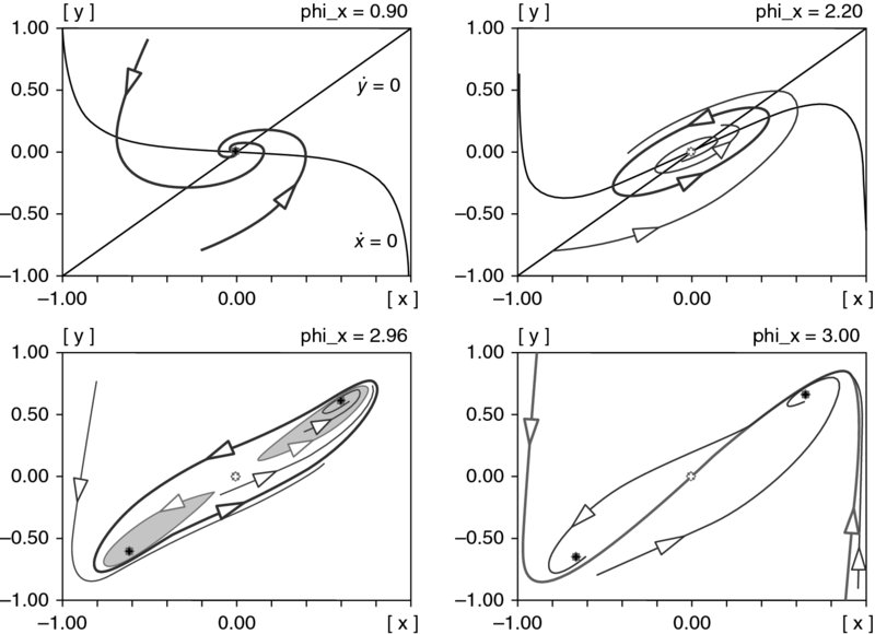
The equilibrium (xo, yo) and the ![]() isocline are, of course, not affected by the changes in φx. On the other hand, increasing values of this parameter shift the isocline
isocline are, of course, not affected by the changes in φx. On the other hand, increasing values of this parameter shift the isocline ![]() downward to the left of the equilibrium and upward to the right of it. The counterclockwise motions are maintained, but at our second value φx = 2.20, they locally spiral outward, that is, the equilibrium has become unstable. Nevertheless, further away from the equilibrium, the centripetal forces prove dominant and generate spirals pointing inward. As a consequence, there must be one orbit in between that neither spirals inward nor outward. Such a closed orbit is indeed unique and constitutes a limit cycle that globally attracts all trajectories, wherever they start from (except the equilibrium point itself). This situation is shown in the top-right panel of Figure 1.
downward to the left of the equilibrium and upward to the right of it. The counterclockwise motions are maintained, but at our second value φx = 2.20, they locally spiral outward, that is, the equilibrium has become unstable. Nevertheless, further away from the equilibrium, the centripetal forces prove dominant and generate spirals pointing inward. As a consequence, there must be one orbit in between that neither spirals inward nor outward. Such a closed orbit is indeed unique and constitutes a limit cycle that globally attracts all trajectories, wherever they start from (except the equilibrium point itself). This situation is shown in the top-right panel of Figure 1.
If φx increases sufficiently, the shifts of the ![]() isocline are so pronounced that it cuts the straight line at two (but only two) additional points (x1, y1) and (x2, y2). One lies in the lower-left corner and the other symmetrically in the upper-right corner of the phase diagram. First, over a small range of φx, these outer equilibria are unstable, after that, for all φx above a certain threshold, they are always locally stable. The latter case is illustrated in the bottom-left panel of Figure 1, where the parameter has increased to φx = 2.96 (the isoclines are not shown here, so as not to overload the diagram).
isocline are so pronounced that it cuts the straight line at two (but only two) additional points (x1, y1) and (x2, y2). One lies in the lower-left corner and the other symmetrically in the upper-right corner of the phase diagram. First, over a small range of φx, these outer equilibria are unstable, after that, for all φx above a certain threshold, they are always locally stable. The latter case is illustrated in the bottom-left panel of Figure 1, where the parameter has increased to φx = 2.96 (the isoclines are not shown here, so as not to overload the diagram).
The two shaded areas are the basins of attraction of (x1, y1) and (x2, y2), each surrounded by a repelling limit cycle. Remarkably, the stable limit cycle from φx = 2.20 has survived these changes; it has become wider, encompasses the two outer equilibria together with their basins of attraction and attracts all motions that do not start there.
The extreme equilibria move towards the limits of the domain of the sentiment variable, x = ±1, as φx increases. They do this faster than the big limit cycle widens. Eventually, therefore, the outer boundaries of the basins of attraction touch the big cycle, so to speak. This is the moment when this orbit disappears, and with it all cyclical motions. The bottom-right panel of Figure 1 for φx = 3.00 demonstrates that then the trajectories either converge to the saddle point (xo, yo) in the middle, if they happen to start on its stable arm, or they converge to one of the other two equilibria.
To sum up, whether the obvious, the ‘natural’ equilibrium (xo, yo) is stable or unstable, system (8) shows a broad scope for cyclical trajectories. Furthermore, whether there are additional outer equilibria or not, there is also broad scope for self-sustaining cyclical behaviour, that is, oscillations that do not explode and, even in the absence of exogenous shocks, do not die out, either.
3. Heterogeneity and Animal Spirits in the New-Keynesian Framework
3.1 De Grauwe's Modelling Approach
Given that the New-Keynesian theory is the ruling paradigm in macroeconomics, Paul De Grauwe had a simple but ingenious idea to challenge it: accept the three basic log-linearized equations for output, inflation and the interest rate of that approach, but discard its underlying representative agents and rational expectations. This means that, instead, he introduces different groups of agents with heterogeneous forms of bounded rationality, as it is called.20 Expectations have to be formed for the output gap (the percentage deviations of output from its equilibrium trend level) and for the rate of inflation in the next period. For each variable, agents can choose between two rules of thumbs where, as specified by the DCA, switching between them occurs according to their forecasting performance. De Grauwe speaks of ‘animal spirits’ insofar as such a model is able to generate waves of optimistic and pessimistic forecasts, notions that are excluded from the New-Keynesian world by construction.21
The following three-equation model is taken from De Grauwe (2008a), which is the first in a series of similar versions that have subsequently been studied in De Grauwe (2010, 2011, 2012a,2012b). The term ‘three-equation’ refers to the three laws that determine the output gap y, the rate of inflation π and the nominal rate of interest i set by the central bank. The symbols π⋆ and i⋆ denote the central bank's target rates of inflation and interest, which are known and taken into account by the agents in the private sector.22 All parameters are positive where, more specifically, ay and bπ are weighting coefficients between 0 and 1. Eaggt are the aggregated expectations of the heterogeneous agents using information up to the beginning of the present period t. They are substituted for the mathematical expectation operator Et, the aforementioned rational expectations. Then, the three equations are:
Equation (9) for the output gap is usually referred to as a dynamic IS equation (in analogy to old theories contrasting investment with savings), here in hybrid form, which means that the expectation term is combined with a one-period lag of the same variable.The Phillips curve in (10), likewise in hybrid form, is viewed as representing the supply side of the economy. Equation (11) is a Taylor rule with interest rate smoothing, that is, it contains the lagged interest rate on the right-hand side.23 The terms ϵy, t, ϵπ, t and ϵi, t are white noise disturbances, interpreted as demand, supply and monetary policy shocks, respectively. Qualitatively little would change if some serial correlation were allowed for them.
The aggregate expectations in these equations are convex combinations of two (extremely) simple forecasting rules. With respect to the output gap, De Grauwe considers optimistic and pessimist forecasters, predicting a fixed positive and negative value of y, respectively. With respect to the inflation rate, he distinguishes between agents who believe in the central bank's target and so-called extrapolators, who predict that next period's inflation will be last period's inflation.24 Accordingly, with g > 0 as a positive constant, nopt as the share of optimistic agents regarding output, and ntar as the share of central bank believers regarding inflation, expectations are given by
In other papers, De Grauwe alternatively stipulates so-called fundamental and extrapolative output forecasters, Efuntyt + 1 = 0 and Eexttyt + 1 = yt − 1. However, the dynamic properties of his model are not essentially affected by such a respecification.
The populations shares of the heterogeneous agents are determined by the suitably adjusted discrete choice equations (1) and (2). Denoting the measures of fitness that apply here by Uopt, Upess, Utar and Uext, we have

Conforming to the principle that better forecasts attract a higher share of agents, fitness is defined by the negative (infinite) sum of the past squared prediction errors, where the past is discounted with geometrically declining weights. Hence, with a so-called memory coefficient 0 < ρ < 1, superscripts A = opt, pess, tar, ext and variables z = y, π in obvious assignment,

This specification of the weights ωk makes sure that they add up to unity. The second expression in (14) is an elementary mathematical reformulation. It allows a recursive determination of the fitness, which is more convenient and more precisely computable than an approximation of an infinite series.
Equation (14) completes the model. De Grauwe makes no explicit reference to an equilibrium of the economy (or possibly several of them?) and does not attempt to characterize its stability or instability. He proceeds directly to numerical simulations and then discusses what economic sense can be made of what we see. Depending on the specific focus in his papers, additional computer experiments with some modifications may follow.
A representative simulation run for the present model and similar models is shown in Figure 2. This example, reproduced from De Grauwe (2008a, p. 24), plots the time series of the output gap (upper panel) and the share of optimistic forecasters (lower panel). The underlying time unit is one month, that is, the diagram covers a period of 25 years. The strong raggedness of the output series is indicative of the stochastic shocks that De Grauwe assumes. In fact, the deterministic core of the model is stable and converges to a state with y = 0, π = π⋆ and i = i⋆. Without checking any stability conditions or eigenvalues, this can be inferred from various diagrams of impulse response functions (IRFs) in De Grauwe's work.
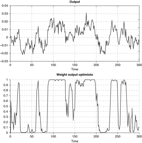
Figure 2. A Representative Simulation Run of Model (9)–(14).
The fluctuations in Figure 2 are therefore not self-sustaining. De Grauwe nevertheless emphasizes that his model generates endogenous waves of optimism and pessimism. This characterization may be clarified by a longer quote from De Grauwe (2010):
These endogenously generated cycles in output are made possible by a self-fulfilling mechanism that can be described as follows. A series of random shocks creates the possibility that one of the two forecasting rules, say the extrapolating one, delivers a higher payoff, that is, a lower mean squared forecast error (MSFE). This attracts agents that were using the fundamentalist rule. If the successful extrapolation happens to be a positive extrapolation, more agents will start extrapolating the positive output gap. The ‘contagion-effect’ leads to an increasing use of the optimistic extrapolation of the output-gap, which in turn stimulates aggregate demand. Optimism is therefore self-fulfilling. A boom is created. At some point, negative stochastic shocks and/or the reaction of the central bank through the Taylor rule make a dent in the MSFE of the optimistic forecasts. Fundamentalist forecasts may become attractive again, but it is equally possible that pessimistic extrapolation becomes attractive and therefore fashionable again. The economy turns around.
These waves of optimism and pessimism can be understood to be searching (learning) mechanisms of agents who do not fully understand the underlying model but are continuously searching for the truth. An essential characteristic of this searching mechanism is that it leads to systematic correlation in beliefs (e.g. optimistic extrapolations or pessimistic extrapolations). This systematic correlation is at the core of the booms and busts created in the model. (p. 12)
Thus, in certain stages of a longer cycle, the optimistic expectations are superior, which increases the share of optimistic agents and enables output to rise, which, in turn, reinforces the optimistic attitude. This mechanism is evidenced by the co-movements of yt and noptt in Figure 2 and conforms to the positive feedback loop highlighted in a comment on the small and stylized system (8) above.25 A stabilizing counter-effect is not as clearly recognizable. De Grauwe only alludes to the central bank's reactions in the Taylor rule, when positive output gaps and inflation rates above their target (which will more or less move together) lead to both higher nominal and real interest rates. This is a channel that puts a curb on yt in the IS equation. In addition, a suitable sequence of random shocks may occasionally work in the same direction and initiate a turnaround.
The New-Keynesian theory is proud of its ‘micro-foundations’. Within the framework of the representative agents and rational expectations, they derive the macroeconomic IS equation (9) and the Phillips curve (10) as log-linear approximations to the optimal decision rules of inter-temporal optimization problems. As these two assumptions have now been dropped, the question arises of the theoretical justification of (9) and (10). Two answers can be given.
First, Branch and McGough (2009) are able to derive these equations invoking two groups of individually boundedly rational agents, provided that their expectation formation satisfies a set of seven axioms.26 The authors point out that the axioms are not only necessary for the aggregation result, but some of them could also be considered rather restrictive; see, especially, Branch and McGough (2009, p. 1043). Furthermore, it may not appear very convincing that the agents are fairly limited in their forecasts, and yet they endeavour to maximize their objective function over an infinite time horizon and are smart enough to compute the corresponding first-order Euler conditions.
Acknowledging these problems, the second answer is that the equations make good economic sense even without a firm theoretical basis. Thus, one is willing to pay a price for the convenient tractability obtained, arguing that more consistent attempts might be undertaken in the future. In fact, De Grauwe's approach also succeeded in gaining the attention of New-Keynesian theorists and a certain appreciation by the more open-minded proponents. This is indeed one of the rare occasions where orthodox and heterodox economists are able and willing to discuss issues by starting out from a common basis.
Branch and McGough (2010) consider a similar version to equations (9)–(11) where, besides naive expectations, they still admit rational expectations. However, the latter are more costly, meaning that they may be outperformed by boundedly rational agents in tranquil times, in spite of their systematic forecast errors. For greater clarity, the economy is studied in a deterministic setting (hence rational expectations amount to perfect foresight). The authors are interested in the stationary points of this dynamics: in general, there are multiple equilibria and the questions is which are stable/unstable, and what are the population shares prevailing in them.
Branch and McGough's analysis provides a serious challenge for the rational expectations hypothesis. Its recommendation to monetary policy is to guarantee determinacy in models of this type (this essentially amounts to the Taylor principle, according to which the interest rate has to rise more than one-for-one with inflation). Branch and McGough illustrate that, in their framework, the central bank may unwittingly destabilize the economy by generating complex (‘chaotic') dynamics with inefficiently high inflation and output volatility, even if all agents are initially rational. The authors emphasize that these outcomes are not limited to unusual calibrations or a priori poor policy choices; the basic reason is rather the dual attracting and repelling nature of the steady-state values of output and inflation.
Anufriev et al. (2013) abstract from output and limit themselves to a version of (10) with only expected inflation on the right-hand side. Since there is no interest rate smoothing in their Taylor rule (c1 = 0) and, of course, no output gap either, the inflation rate is the only dynamic variable. These simplifications allow the authors to consider greater variety in the formation of expectations and to study their effects almost in a vacuum. In this case, too, the main question is whether, in the absence of random shocks, the system will converge to the rational expectations equilibrium. This is possible but not guaranteed because, again, certain ecologies of forecasting rules can lead to multiple equilibria, where some are stable and give rise to intrinsic heterogeneity.
Maintaining the (stochastic) equations (9) and (10) (but without the lagged variables on the right-hand side) and considering different dating assumptions in the Taylor rule (likewise without interest rate smoothing), Branch and Evans (2011) obtain similar results, broadly speaking. They place particular interest in a possible regime-switching of the output and inflation variances (an important empirical issue for the US economy), and in the implications of heterogeneity for optimal monetary policy.
Dräger (2016) examines the interplay between fully rational (but costly) and boundedly rational (but costless) expectations in a subvariant of the New-Keynesian approach, which is characterized by a so-called rational inattentiveness of agents. As a result of this concept, entering the model equations for quarter t are not only contemporary but also past expectations about the variables in quarter t + 1. The author's main concern is with the model's ability to match certain summary statistics and, in particular, the empirically observed persistence in the data. Not the least due to the flexible degree of inattention, which is brought about by the agents’ switching between full and bounded rationality (in contrast to the case where all agents are fully rational, when the degree is fixed), the model turns out to be superior to the more orthodox model variants.27
3.2 Modifications and Extensions
The attractiveness of De Grauwe's modelling strategy is also shown by a number of papers that take his three-equation model as a point of departure and combine it with a financial sector. To be specific, this means that a financial variable is added to equation (9), (10) or (11), and that the real economy also feeds back on financial markets via the output gap or the inflation rate. It is here a typical conjecture, which then needs to be tested, that a financial sector tends to destabilize the original model in some sense; for example, output or inflation may become more volatile.
An early extension of this kind is the integration of a stock market in De Grauwe (2008b). He assumes that an increase in stock prices has a positive influence on output in the IS equation and a negative influence on inflation in the Phillips curve (the latter because this reduces marginal costs). In addition, it is of special interest that the central bank can try to lean against the wind by including a positive effect of stock market booms in its interest rate reaction function. The stock prices are determined, in turn, by expected dividends discounted by the central bank's interest rate plus a constant markup. The actual dividends are a constant fraction of nominal GDP, that is, their forecasts are closely linked to the agents’ forecasts of output and inflation.
In a later paper, De Grauwe and Macchiarelli (2015) include a banking sector in the baseline model. In this case, the negative spread between the loan rate and the central bank's short-term interest rate enters the IS equation in order to capture the cost of bank loans. Along the lines of the financial accelerator by Bernanke et al. (1999), banks are assumed to reduce this spread as firms' equity increases which, by hypothesis, moves in step with their loan demand. Besides yt, πt and it, the model contains private savings and the borrowing-lending spread as two additional dynamic variables. In the final sections of the paper, the model is extended by introducing variable share prices and determining them analogously to De Grauwe (2008b).
De Grauwe and Gerba (2015a) is a very comprehensive contribution that starts out from De Grauwe and Macchiarelli (2015), but specifies a richer structure of the financial sector, which also finds its way into the IS equation. One consequence of the extension is that capital now shows up as another dynamic variable, and that new types of shocks are considered.28 Once again, the discrete choice version is contrasted to the world with rational expectations. In a follow-up paper, De Grauwe and Gerba (2015b) introduce a bank-based corporate financing friction and evaluate the relative contribution of that friction to the effectiveness of monetary policy. On the whole, it is impressive work, but, given the long list of numerical parameters to set, readers have to place their trust in it.
Lengnick and Wohltmann (2013) and, in a more elaborated version, Lengnick and Wohltmann (2016) choose a different approach to add a stock market to the baseline model.29 There are two channels through which stock prices affect the real side of the economy. One is a negative influence in the Phillips curve, which is interpreted as an effect on marginal cost, the other is the difference between stock price and goods price inflation in the IS equation, which may increase output. The modelling of the stock market, on the other hand, is borrowed from the burgeoning literature on agent-based speculative demands for a risky asset. Such a market is populated by fundamentalist traders and trend chasers who switch between these strategies analogously to (13) and (14). The market is now additionally influenced by the real sector through the assumption that the fundamental value of the shares is proportional to the output gap. Furthermore, besides speculators, there is a stock demand by optimizing private households, which increases with output and decreases with the interest rate and higher real stock prices.
While in the simulations, the authors maintain the usual quarter as the length of the adjustment period in (9)–(11)) for the real sector, they specify financial transactions on a daily basis and use time aggregates for their feedback on the quarterly equations. Even in isolation and without random shocks, the stock market dynamics is known for its potential to generate endogenous booms and busts. The spillover effects can now cause a higher volatility in the real sector. For example, it can modify the original effects of a given shock in the IRFs and make them hard to predict.30 One particular concern of the two papers is a possible stabilization through monetary policy, another is a taxation of the financial transactions or profits. An important issue is whether a policy that is effective under rational expectations can also be expected to be so in an environment with heterogeneous and boundedly rational agents.
Scheffknecht and Geiger's (2011) modelling is in a similar spirit (including the different time scales for the real and financial sector), but limits itself to one channel from the stock market to the three-equation baseline specification. To this end, the authors add a risk premium ζt (i.e. the spread between a credit rate and it) to the short-term real interest rate in (9). The transmission is a positive impact of the change in stock prices on ζt, besides effects from yt, it and the volatilities (i.e. variances) of yt, πt, it on this variable.
A new element is an explicit consideration of momentum traders' balance sheets (but only of theirs, for simplicity). They are made up of the value of the shares they hold and money, which features as cash if it is positive and debt if it is negative. This brings the leverage ratios of these traders into play, which may constrain them in their asset demands. Although the latter extension is not free of inconsistencies, these are ideas worth considering.31
4. Herding and Objective Determinants of Investment
The models discussed so far were concerned with expectations about an economic variable in the next period. Here, a phenomenon to which an expression like ‘animal spirits’ may apply occurs when the agents rush towards one of the two forecast rules. However, this behaviour is based on objective factors, normally publicly available statistics. Most prominently, they contrast expected with realized values and then evaluate the forecast performance of the rules.
In the present section, we emphasize that the success of decisions involving a longer time horizon, in particular, cannot be judged from such a good or bad prediction, or from corresponding profits in the next quarter. It takes several years to know whether an investment in fixed capital, for example, was worth undertaking. Furthermore, decisions of that kind must, realistically, take more than one dimension into account. As a consequence, expectations are multi-faceted and far more diffuse in nature. Being aware of this, people have less confidence in their own judgement and the relevance of the information available to them. In these situations, the third paragraph of the Keynes quotation in the introductory section becomes relevant, where he points out that ‘we endeavor to conform with the behavior of the majority or the average’, which ‘leads to what we may strictly term a conventional judgment’. In other words, central elements are concepts such as a (business or consumer) sentiment or climate, or a general state of confidence. In the language of tough business men, it is not only their skills, but also their gut feelings that make them so successful.
Therefore, as an alternative to the usual focus on next-period expectations of a specific macroeconomic variable, we may formulate the following axiom: long-term decisions of the agents are based on sentiment, where, as indicated by Keynes, with agents' orientation towards the behaviour of the majority, this expression may also connote herding. In terms of ‘animal spirits’, we propose that in the models under consideration so far, we have animal spirits in a weak sense, whereas in the context outlined above we have animal spirits in a strong sense; animal spirits proper, so to speak.32
The discrete choice and TPAs can also be used to model animal spirits in the strong sense. Crucial for this is specifying arguments with which the probabilities are supposed to vary, that is, specifying what was called the fitness function or switching index, respectively. Such arguments may neglect an evaluation of short-term expectations, and they should provide a role for herding or contagion. The latter can be achieved conveniently by including a majority index, such that the more agents adhere to one of the attitudes, the higher ceteris paribus the probability that agents will choose it or switch to it.
In the following, we present a series of papers that follow this strategy. What they all have in common is that they pursue the TPA, and that their sentiment variable refers to the fixed investment decisions of firms. The models are thus concerned with a business sentiment. This variable is key to the dynamics because, acting via the Keynesian multiplier, investment and its variations are the driving forces of the economy; other components of aggregate demand play a passive role. Also, all of these models are growth models, a feature that makes them economically more satisfactory than most of the (otherwise meritorious) models described in the previous sections, which are stationary in the long run.
Let us therefore begin by specifying investment and the goods markets. Individual firms have two (net) investment options. These options are given by a lower growth rate of the capital stock ![]() , at which firms invest if they are pessimistic, and a higher growth rate
, at which firms invest if they are pessimistic, and a higher growth rate ![]() , corresponding to an optimistic view of the world. Let go be the mean value of the two,
, corresponding to an optimistic view of the world. Let go be the mean value of the two, ![]() , and x the sentiment of the firms as it was defined in Section 2.2, that is, the difference between optimistic and pessimistic firms scaled by their total number. Hence the aggregate capital growth rate is given by33
, and x the sentiment of the firms as it was defined in Section 2.2, that is, the difference between optimistic and pessimistic firms scaled by their total number. Hence the aggregate capital growth rate is given by33
Being in a growth framework, economic activity is represented by the output-capital ratio u, which can also be referred to as (capital) utilization. Franke (2008a, 2012a) models the other components of demand such that, supposing continuous market clearing, IS utilization is a linear function of (only) the business sentiment,
where σ is the marginal aggregate propensity to save and βu a certain positive, structurally well-defined constant. A consistency condition can (but need not) ensure that a balanced sentiment x = 0 prevails in a steady-state position.
For one part, the specification of the switching index includes the sentiment variable x, which can capture herding. The choice and influence of a second variable revolves around the rest of the economy. Franke (2008a) combines the sentiment dynamics with a Goodwinian struggle between capitalists and workers for the distribution of income. It is summarized in a real wage Phillips curve depending, in particular, on utilization u = u(x) from (16). In this way, the wage share v becomes the second dynamic variable besides x. With a few simple manipulations, its changes can be described by
(βv > 0 another suitable constant). Regarding the sentiment, the idea is that ceteris paribus the firms tend to be more optimistic when the profit share increases (the wage share decreases). With two coefficients φx, φv > 0 and the equilibrium wage share vo, the switching index is thus of the form,34
As derived in Section 2.2, equation (7), the sentiment adjustments read as follows (with β = 2ν = 1),
To sum up, taking account of (18), the economy is reduced to two differential equations in the sentiment x and the wage share v. It could be characterized as a micro-founded Goodwinian model that, besides the innovation of the notion of business sentiment, includes a variable output-capital ratio and an investment function (the latter two features are absent in Goodwin's (1967) original model).
It may be observed that equations (17)–(19) have the same structure as system (8), apart from the slight distortions by cosh ( · ) in (19) and the multiplication of x by v(1 − v) in (17). Therefore, depending on φx, the isocline ![]() resembles the two upper panels of Figure 1, whereas the other isocline
resembles the two upper panels of Figure 1, whereas the other isocline ![]() becomes a vertical line at x = 0. The latter rules out the multiple equilibria in the other two panels of Figure 1.
becomes a vertical line at x = 0. The latter rules out the multiple equilibria in the other two panels of Figure 1.
The dynamic properties are as described in the discussion of (8): the (unique) steady state is locally and globally stable if the herding coefficient φx is less than unity. Otherwise it is repelling, where the reflecting boundaries x = ±1 and the multiplicative factor v(1 − v) in (17) ensure that the trajectories remain within a compact set. Hence (by the Poincaré–Bendixson theorem), all trajectories must converge to a closed orbit. Numerically, by all appearances, it is unique. Accordingly, if (and only if) herding is sufficiently strong, the economy enters a uniquely determined periodic motion in the long run. Regarding income distribution, it features the well-known Goodwinian topics, regarding the sentiment, phases of optimism give way periodically to phases of pessimism and vice versa.
Franke (2012a) specifies the same demand side (15) and (16). Its other elements are:
- A central bank adopting a Taylor rule to set the rate of interest; that is, the interest rate increases in response to larger deviations of utilization from normal and larger deviations of the inflation rate from the bank's target.
- A price Phillips curve with a so-called inflation climate πc taking the role of its expectation term.
- An adjustment equation for the inflation climate, which is a weighted average of adaptive expectations and regressive expectations. The latter means that agents trust the central bank to bring inflation back to target (correspondingly, the weight of these expectations can be interpreted as the central bank's credibility).35
In spite of its structural richness, the economy can be reduced to two differential equations in the sentiment x and the inflation climate πc. As a matter of fact, identifying πc with y, the system has the same form as equation (8) in Section 2 (apart from the cosh term). Therefore, because of its business sentiment and, again, if herding is strong enough, the model can be viewed as an Old-Keynesian version of the interplay of output, inflation and monetary policy, or (in a somewhat risky formulation) of the macroeconomic consensus.36
For situations in which agents carry an asset forward in time, there is a problem with the transition probability and DCA alike, which should not be concealed. It arises from the fact that, with the switching between high and low growth rates in the investment decisions, the capital stocks of individual firms change from one period to another (in absolute and relative terms). On the other hand, the definition of the aggregate capital growth rate in (15) together with the macroscopic adjustment equation for the sentiment x implicity presupposes that the groups of optimistic and pessimistic firms always have the same distribution of capital stocks. As a consequence, these equations are only an approximation. Apart from the size of the approximation errors, acknowledging this feature leads to the question of whether the errors may also accumulate in the course of time.
Yanovski (2014) goes back to the micro-level of the TPA to inquire into this problem. Considering a finite population, he models each firm and its probability calculus individually and also keeps track of the capital stocks resulting from these decisions (modelling that requires a few additional specifications to be made for the micro-level). In short, the author finds that the approximation problem does not appear to be very serious. Of course, every macro-model that uses the transition probability or DCA must be reviewed separately, but this first result is encouraging.
Interestingly, Yanovski discovers another problem, which concerns the size distribution of capital stocks: it tends to be increasingly dispersed over time. The result that some firms become bigger and bigger may or may not be attractive. Yanovski subsequently tries several specification details that may entail a bounded width of the size distribution in the long run. To them, it is crucial to relax the assumption of uniform transition probabilities, and that additional, firm-specific arguments are proposed to enter them. Within a parsimonious framework, these discussions can provide a better understanding of the relationships between micro and macro.37
Going back to macrodynamics, Lojak (2015) adds a financial side to the monetary policy and output-inflation nexus in Franke (2012a). Besides the different saving propensities for workers and rentiers households, which yield a more involved IS equation for goods market clearing, it makes the firms' financing of fixed investment explicit. This work distinguishes between internal sources, that is, the retained earnings of the firms, and external sources, that is, their borrowing from the rentiers (possibly with commercial banks as intermediates). In this way, a third dynamic variable is introduced into the model, the firms' debt-to-capital ratio. It feeds back on the real sector by a negative effect of higher indebtedness on the switching index for the business sentiment x (which again demonstrates the flexibility of this concept).
Motivated by the discussion of Minskian themes in other macro models, the author concentrates on cyclical scenarios and here, in particular, on the co-movements of the debt-asset ratio. While it is usually taken for granted that it lags capital utilization, the author shows that this is by no means obvious. This finding is an example of the need to carefully re-consider the dynamic features of a real-financial interaction.
In a follow-up paper, Lojak (2016) fixes the inflation rate for simplicity and drops the assumption of a constant markup on the central bank's short-term interest rate to determine the loan rate. Instead, the markup is now supposed to increase with the debt-asset ratio, d. This straightforward extension gives rise to additional strong non-linearities. Most amazingly, in the original cyclical scenario of the two-dimensional (x, d) dynamics, a second equilibrium with lower utilization and higher indebtedness comes into being (but not three as in Figure 1). It is also characterized by a locally stable limit cycle around it. The limit cycle around the ‘normal’ equilibrium is maintained, so that two co-existing cyclical regimes are obtained. Not all of the phenomena that one can here observe are as yet fully understood, which shows that it is work in progress and a fruitful field for further investigations. In particular, future research may consider the lending of commercial banks in finer detail, and animal spirits may then play a role in this sector as well.
5. Empirical Validation
Even if the discrete choice and transition probabilities are reckoned to be a conceptually attractive approach for capturing a sentiment dynamics, these specifications would gain in significance if it can be demonstrated that they are compatible with what is observed in reality, or inferred from it. A straightforward attempt to learn about people's decision-making are controlled experiments with human subjects in the laboratory. Regarding empirical testing in the usual sense, there are two different ways to try, a direct and a more indirect way. The first method treats a sentiment adjustment equation such as (3) or (5) as a single-equation estimation, where the variable xt in (5) or the population shares n+t, n−t in (3) are proxied by an economic survey. In fact, several such surveys provide so-called sentiment or climate indices. The second method considers a model as a whole and seeks to estimate its parameters in one effort. Here, however, x or n+, n− remain unobserved variables, that is, only ‘normal’ macroeconomic variables such as output, inflation, etc., are included as empirical data. These three types of a reality check are considered in the following subsections.
5.1 Evidence from the Lab
Self-inspection is not necessarily the best method to find out how people arrive at their decisions. A more systematic way that approaches people directly in this matter are laboratory experiments. To begin with, they indeed provide ample evidence that the subjects use similarly simple heuristics to those considered in the models that we have presented; see Assenza et al. (2014a) for a comprehensive literature survey. A more specific point is whether the distribution of different rules within a population and its changes over time could be explained by the discrete choice or TPA. Several experiments at CeNDEF (University of Amsterdam) allow a positive answer with respect to the former. In the setting of a New-Keynesian three-equation model, Assenza et al. (2014b) find four qualitatively different macro-patterns emerging out of a self-organizing process where one of four forecasting rules tends to become dominant in the consecutive rounds of an experiment. The authors demonstrate that this is quite in accordance with the discrete choice principle.38
In another study by Anufriev et al. (2016), where the series to be forecasted are exogenously generated prior to the experiments and the subjects have to choose between a small numbers of alternatives given to them, a discrete choice model can in most cases be successfully fitted to the subjects' predictions. In particular, the experimenters can make inference about the intensity of choice, although different treatments yield different values. For all of these studies, however, it has to be taken into account that a full understanding of the results requires the reader to get involved in a lot of details.
5.2 Empirical Single-Equation Estimations
With respect to inference from empirical data, let us first consider surveys collecting information about the expectations or sentiment of a certain group in the economy. As far as we know, the first empirical test of this kind is Branch (2004). He is concerned with the Michigan survey where private households are asked on a monthly basis for their expectations about future inflation. For his analysis, the author equips the respondents with three virtual predictor rules: naive (i.e. static) expectations, adaptive expectations and the relatively sophisticated expectations obtained from a vector autoregression (VAR) that besides inflation includes unemployment, money growth and an interest rate. The fitness of these rules derives from the squared forecast errors and a specific cost term (which has to be re-interpreted after the estimations).
The model thus set up is estimated by maximum likelihood. The estimate of the intensity of choice is significantly positive, such that all three rule are relevant (even the naive expectations) and their fractions exhibit non-negligible fluctuations over time. It is also shown that this model is markedly superior to two alternatives that assume the forecasts are normally distributed around their constant or time-varying mean values across the respondents.
Branch (2007) is a follow-up paper using the same data. Here, the forecast rules entering the discrete choice model are more elaborate than in his earlier paper. They are actually based on explanations from a special branch of the New-Keynesian literature (which uses the concept of limited information flows as it was developed in Mankiw and Reis, 2002). Thus, heterodox economists will probably not be very convinced by this theory. Nevertheless, the heterogeneity and switching mechanism introduced into the original New-Keynesian model with its homogeneous agents prove to be essential as this version provides a better fit of the data.
Several other business and consumer surveys lend themselves for testing theoretical approaches with binary decisions, because they already ask whether respondents are ‘optimistic’ or ‘pessimistic’ concerning the changes of a variable or the entire economy. To accommodate the possibility that a third, neutral assessment is also usually allowed for, it is assumed that neutral subjects can be assigned half and half to the optimistic and pessimistic camp. Franke (2008b) is concerned with two leading German surveys conducted by the Ifo Institute (Ifo Business Climate Index) and the Center for European Research (ZEW Index for Economic Sentiment), both of which are available at monthly intervals.
The respondents are business people and financial analysts, respectively. Because they are asked about the future prospects of the economy, the aggregate outcome can be viewed as a general sentiment prevailing in these groups. Given the theoretical literature discussed above, this suggests testing the TPA with a herding component included. Franke formulates the corresponding sentiment changes in discrete time and extends equation (5) and its switching index somewhat beyond what has been considered so far:
where xt is the Ifo or ZEW index, respectively, and yt is the detrended log series of industrial production (the output gap, in percent). Compared to previous discussions, three generalizations are allowed for in the switching index. (i) The coefficient φo measures a possible predisposition to optimism (if it is positive) or pessimism (if it is negative). (ii) In addition to the levels of x and y, first differences of the two variables can account for momentum effects. In particular, herding has two aspects: joining the majority (represented by φx), and immediate reactions to changes in the composition of the sentiment, which Franke (2008b, p. 314) calls the moving-flock effect. (iii) There may be lags Δτ (τ = 1, 2, …,) in the first differences.
The intrinsic noise from the probabilistic decisions of a finite number of agents is neglected. Instead, the stochastic term ϵx, t represents random forces from outside the theoretical framework, that is, extrinsic noise. Thus, (20) can be estimated by non-linear least squares (NLS), with ϵx, t as its residuals.
In the estimations of (20), a number of different cases were explored. Skipping the details and turning directly to the most efficient version where all of the remaining coefficients were well identified, a herding mechanism was indeed revealed for both indices. The majority effect, however, was of secondary importance and could be justifiably dismissed from the model (i.e. φx = 0), so that herding was best represented by the moving-flock effect.
The arrival of new information on economic activity also plays a role. Relevant for both indices is again the momentum effect, while the level effect can be discarded for one index. Remarkably, the coefficient φy is negative when it is included (even in the version where φΔy is set equal to zero). A possible interpretation is that subjects in a boom already anticipate the subsequent downturn. Since it may not appear entirely convincing, the negative φy could perhaps be better viewed as a mitigation of the procyclical herding effect.
The finding of a strong role for the moving-flock effect is a challenge for theoretical modelling because incorporating it into our continuous-time framework would easily spoil a model's otherwise relatively simple mathematical structure. It would also affect its dynamic properties to some extent. The somewhat inconvenient features are discussed and demonstrated in Franke (2008a, pp. 249ff), but the issue has not been taken up in the following literature.
Subsequent to these results, Franke (2008b) considers two extensions of the estimation approach (20). First, he tests for cross-effects between the two indices, where he finds that the changes in the Ifo index (though not the levels) influence the respondents of the ZEW index, but not the other way around. This makes sense, given the specific composition of the two groups. The second extension tests for an omitted variable of unknown origin. This can be achieved by adding a stochastic variable zt to the switching index in (20) and supposing, for simplicity, that its motions are governed by a first-order autoregressive process. Such a specification allows an estimation by maximum likelihood together with the Kalman filter, which serves to recover the changes in zt. Again, an improvement is found for one index but not the other.
Lux (2009) uses the ZEW survey to estimate the TPA with an alternative and more elaborate method. To this end, he goes back to the micro-level and invokes the statistical mechanics apparatus, basically in the form of the Fokker–Planck equation in continuous time. In this way, he is able to derive the conditional transitional probability densities of the sentiment variable xt between two months, and thus compute, and maximize, a likelihood function. The main conceptual difference in this treatment from the NLS estimation is that it makes no reference to extrinsic noise. Instead, it includes the intrinsic noise, so that it can also determine the finite number of ‘autonomous’ subjects in the sample.
The results are largely compatible with the references made about Franke (2008b). The likelihood estimation is potentially superior because it seeks to exploit more information, albeit at the cost of considerably higher computational effort. Ideally, NLS may be employed at a first stage to identify promising specifications, which then form the basis for more precise conclusions at a second stage.
In sum, it can be concluded from the two investigations by Franke and Lux that the TPA is a powerful explanation for the ups and downs in the expectation formation of the respondents in the two surveys, which does not need to rely on unobservable information shocks. For this good result, however, the specifications in the switching index are slightly more involved than in our theoretical discussions.
Ghonghadze (2016) recently conducted an NLS estimation in the spirit of equation (20) on a survey of senior loan officers regarding their bank lending practices. The respondents were asked whether they raised versus lowered the spreads between loan rates and banks' costs of funds, that is, a tightening versus an easing of lending terms. This work, too, finds evidence of social interactions within this group, albeit with a view to certain macroeconomic indicators.
Still being concerned with a single-equation estimation, Cornea-Madeira et al. (2017) is a contribution that tests the DCA by referring to empirical macroeconomic data. Their testing ground is the New-Keynesian Phillips curve, where regarding the expectations entering it, the agents can choose between naive forecasts and forecasts derived from an ambitious VAR that in addition to inflation takes account of the output gap and the rate of change of unit labour costs and of the labour share.39 Again, the fitness of the two rules is determined by the past forecast errors. Since the population shares constituting the aggregate expectations can be ultimately expressed as functions of these macroeconomic variables, the Phillips curve can be estimated by NLS.
There are two structural parameters to be estimated, the slope coefficient for the marginal costs and the intensity of choice in the switching mechanism. Both of them have the correct positive sign at the usual significance levels. Overall, the predicted inflation path tracks the behaviour of actual inflation fairly well. The population share of the naive agents varies considerably over time, although it exhibits a high persistence. Interestingly, their fraction is relatively high or low during certain historical episodes. On average, the simplistic rule is adopted by no less than 67% of the agents.
The authors furthermore test this model against a number of alternatives, two of which are closely related to versions from the New-Keynesian estimation literature. All of them are rejected at a 95% confidence level. Also, robustness checks regarding alternative specifications of the VAR forecasting model and different empirical measures of marginal costs are undertaken. They show no need for any qualification of the previous conclusions. In sum, these results are a strong point in favour of the agents' heterogeneity plus a discrete choice switching mechanism.
The model investigated by Cornea-Madeira et al. (2017) may win another point because of its parsimony. On the other hand, a model with more parameters may be conceptually more satisfactory. Generally, modelling faces a trade-off between econometric efficiency and rich economic structure. For each single (non-trivial) case, this is a difficult problem of judgement, intuition and preferences.
5.3 System Estimations
A second estimation approach is concerned with an entire model into which a sentiment dynamics has been integrated. Accordingly, it seeks to estimate the parameters of the latter together with the parameters in the rest of the model, that is, it is about testing a joint hypothesis. While in the New-Keynesian mainstream literature, the dominant and widely applied system estimation method is Bayesian likelihood estimation, it is fraught with two difficulties: the model must have been linearized and it does not admit unobservable variables. Otherwise the mathematical and computational effort increases, and prohibitively so for non-specialists.
An alternative method can easily cope with these problems. It departs from the truism that no model can capture all aspects of the real world and that every model is built for a specific purpose. Therefore, a model is good if it fulfills its purpose; failures in other directions can and need to be tolerated. In the present context, a ‘purpose’ is given by a number of properties, often referred to as ‘stylized facts’, which can be filtered from reality and that researchers wish to be displayed in their models. Generally, these properties are quantified as summary statistics, which in econometric language are also called ‘moments’.
A model will be unable to reproduce the desired empirical moments perfectly. Estimation means searching for parameter values such that the moments generated by the model come as close as possible to their empirical counterparts. Since a model usually has to be simulated to obtain these moments, one speaks of the method of simulated moments.
The crucial point is, of course, the choice of moments, which a number of econometric critics brand as arbitrary. It can, however, be argued that this feature is a virtue rather than a vice, because it requires researchers to be explicit about their priorities; readers can then decide whether they share or accept them. While in the present wording, a likelihood function can be said to take ‘all moments’ into account, this concept presupposes that the model is correctly specified. If, on the other hand, it is recognized that a model (by definition) is an abstract approximation to reality, then a discussion of the choice of the moments underlying an estimation appears to be more transparent.40
The moments can, moreover, provide a useful diagnosis for a model. By finding out that some moments are relatively well matched and that others are not, one learns more about the merits and demerits of a model than knowing that an objective function (be it a likelihood or something else) has been optimized, and perhaps having a technical econometric measure to summarize the goodness-of-fit.
Franke (2012b, 2016) applies the method of simulated moments to several discrete-time versions of Franke's (2012a) ‘Old-Keynesian’ model of the macroeconomic consensus with its three observable variables: quarterly output, inflation and the interest rate (all of them as percentage deviations from trend). The empirical moments employed are the variances and cross-covariances of these variables in the US economy with lags up to eight quarters, which gives a total of 78 statistics. Their informational value is, however, lower since the moments are not independent.
One of the model versions considered is a deterministic system; one has stochastic demand, cost push and monetary policy shocks added in the corresponding equations; a third version additionally allows two of them to take effect in the switching index and the adjustments of the inflation climate. Thus, nine parameters are to be estimated in the first and 14 parameters in the third version. Such a large number relative to the number of ‘effective’ moments requires great care in the minimization of the objective function that measures the distance between simulated and empirical moments, because it will typically have multiple local minima or extended valleys. The latter phenomenon will also deteriorate the precision of the parameter estimates (unless one chooses to fix some of them on the basis of other arguments or priorities). However, these problems would apply equally well to likelihood methods.
With respect to the so-called period of the Great Moderation (1982 – 2007), the thin (blue) solid line in Figure 3 illustrates that already the deterministic model achieves a respectable matching of the covariance profiles (recall that lags higher than eight quarters are not included in the estimation). The shaded areas indicate that the great majority of the model-generated moments lie inside the 95% confidence band of the empirical moments. The match is even better in the full stochastic version; see the bold (red) solid lines in the diagram.41 However, a certain price must be paid for this improvement: the influence of the stochastic dynamics becomes so strong that the herding coefficient in the switching index (the analogue of φx in (18)) is relatively low and would imply stability of the steady state in the deterministic core of the model. In other words, it is the random shocks that keep the system in motion. Regarding the period of the Great Inflation (1960–1979), the coefficient is even close to zero.
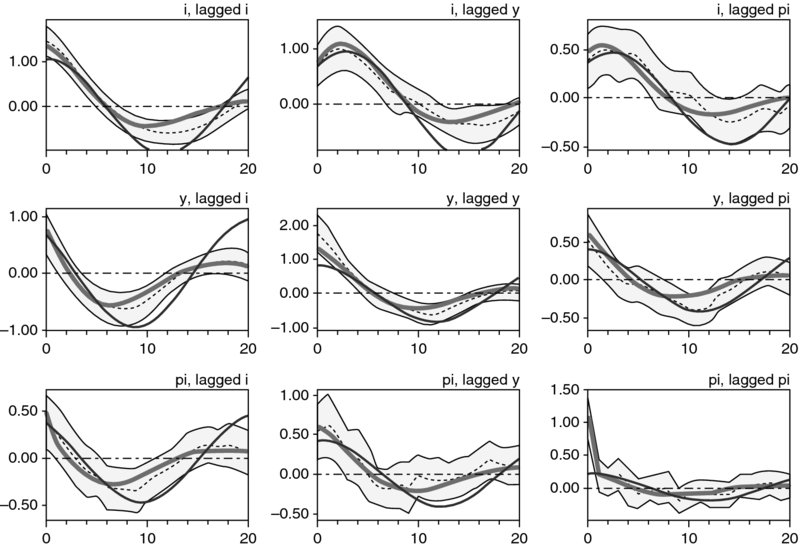
Figure 3. Auto- and Cross-Covariance Profiles of the Estimated ‘Old-Keynesian’ Model in Franke (2012b).
Note: y, pi and i designate the gaps of output, inflation and the interest rate, respectively. Shaded areas are the bootstrapped 95% confidence bands around the empirical moments (dotted lines). Other lines are explained in the text.
In short, the model achieves a good or almost excellent matching of the chosen moments, which can also be quantitatively established in econometric terms. On the other hand, this result does not confirm the endogeneity of the cyclical behaviour of the economy. With the experience of the single-equation estimations above, one may now wonder about the possible presence of the so-called moving-flock effect, a question that has not yet been addressed in any master or PhD thesis.
An additional matter of concern in Franke's (2012b, 2016) contribution is the competitiveness of his model versus a corresponding (hybrid) New-Keynesian model (equations (9)–(11) with rational expectations in place of the boundedly rational expectations Eagg). Broadly speaking, both models are found to be equally successful at reproducing the auto-covariances of their three state variables. If one is more ambitious, however, it has to be noted that the auto-covariances and the raggedness of the inflation rate can hardly be reconciled in the New-Keynesian model: either it produces a good match of the former and a bad match of the latter, or vice versa. In the Old-Keynesian model, by contrast, the two types of moments are largely compatible, that is, a good match of one type may exist alongside at least an acceptable match of the other type. In this sense, the Old-Keynesian model may claim to do a better job.
Using Euro Area data and the same 78 second moments as Franke, the authors Jang and Sacht (2016a) estimate De Grauwe's model (with identically distributed shocks added) by the method of simulated moments. Regarding the coefficients in the discrete choice switching mechanism, they argue in favour of exogenously fixing a moderate intensity of choice β = 1 in (13) and a zero memory coefficient ρ = 0 in (14).42 They furthermore provide detailed information about several other parameters. Especially the estimates of the monetary policy coefficients make good economic sense. At least to the naked eye, the matching itself is of a similar quality as in Figure 3, and slightly superior to the matching of the model's rational expectations version.43
Jang and Sacht (2016b) continue this line of research. In this paper, they consider four forecast rules (two of which with slightly more ‘momentum’ than before) and alternatively include two, three or all four in the model. Together with the rational expectations, they arrange a horse race for six model versions. With respect to US data and the Euro Area data, it is found in both cases that, when matching the same 78 moments as before, the interaction between the two new (and more dynamic) rules is almost as successful as all four rules together. In fact, insignificant values for the parameters characterizing the other two rules indicate that these are virtually ineffective. This finding supplies new knowledge in the search for efficient and parsimonious specifications within the De Grauwe framework. Besides, the rational expectations perform the worst, which is explained by the assumption of ruling out the lagged variables (i.e. the hybrid case) in equations (9) and (10).
Daring to provide a brief summary of these results, at least from a higher point of view and as a preliminary conclusion, it seems that the model approaches by Franke and De Grauwe receive similarly good and satisfactory empirical support from estimations by the method of simulated moments.
Another feature that bounded rationality models might possibly better capture than DSGE models are the kurtosis of the output growth rates, on which De Grauwe (2012a) puts great emphasis, or (better) a measure of fat tails in their distribution such as the shape parameter b of the exponential power distribution, which includes the normal distribution with b = 2 as a special case. There is some literature indicating that b is typically less than 2 (e.g. Fagiolo et al., 2008), but Franke (2015) points out that once one separates the Great Moderation from the Great Inflation period, this ‘stylized fact’ is no longer so well founded. That is, it seems the shape parameter can only be measured with a limited empirical precision. It may nevertheless be worthwhile to explore whether this ‘moment’ could improve the existing estimation.
Finally, Brenneisen (2015) starts out from a recent paper by Liu and Minford (2014), who compare a purely forward-looking New-Keynesian model to a (very) simple version of De Grauwe's model. Estimating them by indirect inference, these authors conclude that the former model outperforms the latter. Brenneisen points out a number of unclear points in Liu and Minford's presentation, and then, instead, applies the method of simulated moments to the two models – whereby he arrives at the reverse conclusion. A more differentiated picture is obtained with respect to moderate extensions of the models.
Very informative in Brenneisen's contribution is a methodological issue regarding the precision of the parameter estimates. Distributions of the parameters can be computed by repeatedly re-estimating a model on the bootstrapped empirical moments, which is a sound but extremely time-consuming procedure. The author successfully tests a new econometric proposal for approximating these distributions by simulations of another random distribution, which can do without the re-estimations completely. This alternative device is relatively easy to implement and could prove useful in future applications of the method of simulated moments.
6. Conclusion
With respect to macroeconomics, this survey was concerned with recent attempts to translate aspects of the famous notion of the animal spirits into formal and rigorous modelling. To cope with the ‘wilderness of bounded rationality’, two approaches with a stylized micro-foundation were addressed: the DCA and the TPA. Before discussing their applications in the literature, it was revealed that they are more closely related than it might seem at first glance, and that they are well suited to endogenously generate persistent cyclical behaviour.
The literature presented here shows a considerable flexibility in building macrodynamic models from these tools, or incorporating them into existing models. As a first guideline for finding one's way around the many models, a distinction was offered between animal spirits in a weak sense and in a strong sense. The first expression merely points to a rush towards one of two attitudes, strategies or similar alternatives; the second involves an element of herding because, in a world of irreducible uncertainty, people think the majority knows better. The first variety is typically found in models that work with the DCA. The second can primarily be classified in models applying the TPA. However, this role allocation is based more on historical reasons rather than on a compelling inner logic.
Besides being theoretically attractive, the two approaches were also shown to have some empirical support. Overall, the material and ideas discussed can provide fruitful stimulations for future research that seeks to capture the formation of business or consumer sentiment, or of a general state of confidence, in a serious and structured way. Maybe this survey comes at a good time, before further modelling work in this direction abounds.
Acknowledgement
We wish to thank two anonymous referees for their constructive comments.
Notes
References
- Akerlof, G.A. and Shiller, R.J. (2009) Animal Spirits. Princeton and Oxford: Princeton University Press.
- Alfarano, S. and Lux, T. (2007) A noise trader model as a generator of apparent power laws and long memory. Macroeconomic Dynamics 11(Supplement 1): 80–101.
- Anderson, S., de Palma, A. and Thisse, J. (1993) Discrete Choice Theory of Product Differentiation. Cambridge, MA: MIT Press.
- Anufriev, M., Assenza, T., Hommes, C. and Massaro, D. (2013) Interest rate rules and macroeconomic stability under heterogeneous expectations. Macroeconomic Dynamics 17: 1574–1604.
- Anufriev, M., Bao, T. and Tuinstra, J. (2016) Microfoundations for switching behavior in heterogeneous agent models: An experiment. Journal of Economic Behavior and Organization 129: 74–99.
- Anufriev, M. and Hommes, C. (2012a) Evolutionary selection of individual expectations and aggregate outcomes in asset pricing experiments. American Economic Journal: Microeconomics 4:4: 35–64.
- Anufriev, M. and Hommes, C. (2012b) Evolution of market heuristics. The Knowledge Engineering Review 27: 255–271.
- Assenza, T., Bao, T., Hommes, C. and Massaro, D. (2014a) Experiments on expectations in macroeconomics and finance. In J. Duffy (ed.), Experiments in Macroeconomics (Research in Experimental Economics), Vol. 17 (pp. 11–70). Bingley, West Yorkshire: Emerald Group Publishing Limited.
- Assenza, T., Heemeijer, P., Hommes, C. and Massaro, D. (2014b) Managing self-organization of expectations through monetary policy: A macro experiment. CeNDEF, University of Amsterdam, Working Paper 2014-07.
- Bernanke, B.S., Gertler, M. and Gilchrist, S. (1999) The financial accelerator in a quantitative business cycle framework. In J.B. Taylor and M. Woodford(eds.), Handbook of Macroeconomics, Vol. 1 (pp. 1342–1393). Amsterdam: North-Holland.
- Boyd, I. and Blatt, J.M. (1988) Investment, Confidence and Business Cycles. New York: Springer.
- Branch, W. (2004) The theory of rationally heterogeneous expectations: Evidence from survey data on inflation expectations. Economic Journal 114: 592–621.
- Branch, W. (2007) Sticky information and model uncertainty in survey data on inflation expectations. Journal of Economic Dynamics and Control 31: 245–276.
- Branch, W.A. and Evans, G.W. (2011) Monetary policy and heterogeneous expectations. Economic Theory 47: 365–393.
- Branch, W.A. and McGough, B. (2009) A New Keynesian model with heterogeneous expectations. Journal of Economic Dynamics and Control 33: 1036–1051.
- Branch, W.A. and McGough, B. (2010) Dynamic predictor selection in a new Keynesian model with heterogeneous expectations. Journal of Economic Dynamics and Control 34: 1492–1508.
- Brazier, A., Harrison, R., King, M. and Yates, T. (2008) The danger of inflating expectations of macroeconomic stability: Heuristic switching in an overlapping-generations monetary model. International Journal of Central Banking 4:2: 219–254.
- Brenneisen, J.-N. (2015) Moment matching of heterogeneous expectations in a class of recent macroeconomic business cycle models. Unpublished master thesis, University of Kiel.
- Brock, W.A. and Durlauf, S.N. (2001) Discrete choice with social interactions. Review of Economic Studies 68: 235–260.
- Brock, W.A. and Hommes, C.H. (1997) A rational route to randomness. Econometrica 65: 1059–1095.
- Brock, W.A. and Hommes, C.H. (1998) Heterogeneous beliefs and routes to chaos in a simple asset pricing model. Journal of Economic Dynamics and Control 22: 1235–1274.
- Brock, W.A., Hommes, C.H. and Wagener, F.O.O. (2005) Evolutionary dynamics in markets with many trader types. Journal of Mathematical Economics 41: 7–42.
- Chang, S.-K. (2007) A simple asset pricing model with social interactions and heterogeneous beliefs. Journal of Economic Dynamics and Control 31: 1300–1325.
- Chiarella, C. and Di Guilmi, C. (2015) The limit distribution of evolving strategies in financial markets. Studies in Nonlinear Dynamics and Econometrics 19(2): 137–159.
- Cochrane, J.H. (2001) Asset Pricing. Princeton: Princeton University Press.
- Cornea-Madeira, A., Hommes, C. and Massaro, D. (2017) Behavioral heterogeneity in U.S. inflation dynamics. Journal of Business Economics and Statistics, forthcoming.
- De Grauwe, P. (2008a) DSGE-modelling when agents are imperfectly informed. ECB, Working Paper Series No. 897.
- De Grauwe, P. (2008b) Stock prices and monetary policy. Centre for European Policy Studies, Working Document No. 304.
- De Grauwe, P. (2010) Top-down versus bottom-up macroeconomics. CESifo Working Paper No. 3020.
- De Grauwe, P. (2011) Animal spirits and monetary policy. Economic Theory 47: 423–457.
- De Grauwe, P. (2012a) Booms and busts in economic activity: A behavioral explanation. Journal of Economic Behavior and Organization 83: 484–501.
- De Grauwe, P. (2012b) Lectures on Behavioral Macroeconomics. Princeton, NJ: Princeton University Press.
- De Grauwe, P. and Gerba, E. (2015a) Stock market cycles and supply side dynamics: Two worlds, one vision? CESifo Working Paper No. 5573.
- De Grauwe, P. and Gerba, E. (2015b) Monetary transmission under competing corporate finance regimes. London School of Economics, FinMaP-Working Paper, No. 52.
- De Grauwe, P. and Macchiarelli, C. (2015) Animal spirits and credit cycles. Journal of Economic Dynamics and Control 59: 95–117.
- Diks, C. and van der Weide, T. (2005) Herding, a-synchronous updating and heterogeneity in memory in a CBS. Journal of Economic Dynamics and Control 29: 741–762.
- Dräger, L. (2010) Why don't people pay attention? Endogenous sticky information in a DSGE Model. University of Hamburg, DEP Discussion Papers Macroeconomics and Finance Series 2/2010.
- Dräger, L. (2011) Endogenous persistence with recursive inattentiveness. University of Hamburg, DEP Discussion Papers Macroeconomics and Finance Series 3/2011.
- Dräger, L. (2016) Recursive inattentiveness with heterogeneous expectations. Macroeconomic Dynamics 20: 1073–1100.
- Fagiolo, G., Napoletano, M. and Roventini, A. (2008) Are output growth rate distributions fat-tailed: Evidence for OECD-countries. Journal of Applied Econometrics 23: 639–669.
- Farmer, R. and Guo, J.T. (1994) Real business cycles and the animal spirit hypothesis. Journal of Economic Theory 63: 42–72.
- Flaschel, P., Franke, R. and Semmler, W. (1997) Dynamic Macroeconomics: Instability, Fluctuations, and Growth in Monetary Economies. Cambridge, MA: MIT Press.
- Franke, R. (2008a) Microfounded animal spirits and Goodwinian income distribution dynamics. In P. Flaschel and M. Landesmann (eds.), Effective Demand, Income Distribution and Growth. Research in Memory of the Work of Richard M. Goodwin (pp. 372–398). London: Routledge.
- Franke, R. (2008b) Estimation of a microfounded herding model on German survey expectations. Intervention: European Journal of Economics and Economic Policies 5: 301–328.
- Franke, R. (2012a) Microfounded animal spirits in the new macroeconomic consensus. Studies in Nonlinear Dynamics and Econometrics 16(4): 1–39.
- Franke, R. (2012b) Competitive moment matching of a New-Keynesian and an Old-Keynesian model: Extended version. Working paper, University of Kiel. http://www.gwif.vwl.uni-kiel.de/en/working-papers (Last access July 2017).
- Franke, R. (2014) Aggregate sentiment dynamics: A canonical modelling approach and its pleasant nonlinearities. Structural Change and Economic Dynamics 31: 64–72.
- Franke, R. (2015) How fat-tailed is US output growth? Metroeconomica 66: 213–242.
- Franke, R. (2016) Competitive moment matching of a New-Keynesian and an Old-Keynesian model. Journal of Economic Interaction and Coordination, forthcoming.
- Franke, R. and Westerhoff, F. (2012) Structural stochastic volatility in asset pricing dynamics: Estimation and model contest. Journal of Economic Dynamics and Control 36: 1193–1211.
- Franke, R. and Westerhoff, F. (2017) Taking stock: A rigorous modelling of animal spirits in macroeconomics (Extended version). Working paper, Universities of Kiel and Bamberg.
- Galí, J. (1994) Monopolistic competition, business cycles, and the composition of aggregate demand. Journal of Economic Theory 63: 73–96.
- Ghonghadze, J. (2016) Variation of lending terms and the financial instability hypothesis. Working paper, University of Kiel.
- Goodwin, R.M. (1967) A growth cycle model. In C.H. Feinstein (ed.), Socialism, Capitalism and Growth. Cambridge: Cambridge University Press.
- Hommes, C.H., Huang, H. and Wang, D. (2005) A robust rational route to randomness in a simple asset pricing model. Journal of Economic Dynamics and Control 29: 1043–1072.
- Jang, T.-S. and Sacht, S. (2016a) Animal spirits and the business cycle: Empirical evidence from moment matching. Metroeconomica 67: 76–113.
- Jang, T.-S. and Sacht, S. (2016b) Modelling consumer confidence and its role for expectation formation: A horse race. Working paper, Kyungpook National University and University of Kiel.
- Keynes, J.M. (1936) The General Theory of Employment, Interest and Money. London: Macmillan.
- Keynes, J.M (1937) The general theory of employment. Quarterly Journal of Economics 51: 109–123.
- Kirman, A. (1993) Ants, rationality and recruitment. Quarterly Journal of Economic 108: 137–156.
- Lahkar, R. and Sandholm, W.H. (2008) The projection dynamic and the geometry of population games. Games and Economic Behavior 64: 565–590.
- Lengnick, M. and Wohltmann, H.-W. (2013) Agent-based financial markets and New Keynesian macroeconomics: A synthesis. Journal of Economic Interaction and Coordination 8: 1–32.
- Lengnick, M. and Wohltmann, H.-W. (2016) Optimal monetary policy in a new Keynesian model with animal spirits and financial markets. Journal of Economic Dynamics and Control 64: 148–165.
- Lines, M. and Westerhoff, F. (2010) Inflation expectations and macroeconomic dynamics: The case of rational versus extrapolative expectations. Journal of Economic Dynamics and Control 34: 246–257.
- Liu, C. and Minford, P. (2014) Comparing behavioural and rational expectations for the US post-war economy. Economic Modelling 43: 407–415.
- Lojak, B. (2015) Investor sentiment, corporate debt and inflation in a feedback-guided model of the business cycle. Unpublished master thesis, University of Kiel.
- Lojak, B. (2016) Sentiment-driven investment, non-linear corporate debt dynamics and co-existing business cycle regimes. Metroeconomica (forthcoming).
- Lux, T. (1995) Herd behaviour, bubbles and crashes. Economic Journal 105: 881–889.
- Lux, T. (2009) Rational forecasts or social opinion dynamics: Identification of interaction effects in a business climate index. Journal of Economic Behavior and Organization 72: 638–655.
- Mankiw, N.G. and Reis, R. (2002) Sticky information versus sticky prices: A proposal to replace the New Keynesian Phillips curve. Quarterly Journal of Economics 117: 1295–1328.
- Manski, C. and McFadden, D. (1981) Structural Analysis of Discrete Data with Econometric Applications. Cambridge, MA: MIT Press.
- Massaro, D. (2013) Heterogeneous expectations in monetary DSGE models. Journal of Economic Dynamics and Control 37: 680–692.
- Minsky, H.P. (1975) John Maynard Keynes. New York: Columbia University Press.
- Ochea, M. (2010) Essays on nonlinear evolutionary game dynamics. PhD thesis, University of Amsterdam: Book no. 468 of the Tinbergen Institute Research Series.
- Pecora, N. and Spelta, A. (2017) Managing monetary policy in a New Keynesian model with many beliefs types. Economics Letters 150: 53–58.
- Scheffknecht, L. and Geiger, F. (2011) A behavioral macroeconomic model with endogenous boom-bust cycles and leverage dynamics. FZID Discussion Paper 37-2011, University of Hohenheim.
- Weidlich, W. and Haag, G. (1983) Concepts and Models of a Quantitative Sociology. The Dynamics of Interacting Populations. Berlin: Springer.
- Westerhoff, F. (2006) Business cycles, heuristic expectation formation and contracyclical policies. Journal of Public Economic Theory 8: 821–838.
- Westerhoff, F. and Hohnisch, M. (2007) A note on interactions-driven business cycles. Journal of Economic Interaction and Coordination 2: 85–91.
- Yanovski, B. (2014) Introducing an elementary microstructure into macrodynamic models. Unpublished master thesis, University of Kiel.