
Session Data
Abstract
Session data is the summary of the communication between two network devices. Also known as a conversation or a flow, this summary data is one of the most flexible and useful forms of NSM data. While session data doesn’t provide the level of detail found in full packet capture data, it does have some unique strengths that provide significant value to NSM analysts.
In this chapter we will discuss how flows are generated, methods for session data collection, and explore two of the more popular session data analysis solutions, SiLK and Argus. However, before going into detail about the differences between analysis solutions, it’s important to understand the differences between the types of flow data. This book will highlight the most commonly used flow types, NetFlow and IPFIX.
Keywords
Network Security Monitoring; Collection; Session Data; Flow; NetFlow; IPFIX; Fprobe; YAF; SiLK; Argus; 5-tuple
Chapter Contents
Collecting and Analyzing Flow Data with SiLK
Installing SiLK in Security Onion
Filtering Flow Data with Rwfilter
Collecting and Analyzing Flow Data with Argus
Session data is the summary of the communication between two network devices. Also known as a conversation or a flow, this summary data is one of the most flexible and useful forms of NSM data. If you consider full packet capture equivalent to a recording of every phone conversation someone makes from a their mobile phone, then you might consider session data to be equivalent to having a copy of the phone log on the bill associated with that mobile phone. Session data doesn’t give you the “What”, but it does give you the “Who, Where, and When”.
When session or flow records are generated, the record will usually include the protocol, source IP address and port, the destination IP address and port, a timestamp of when the communication began and ended, and the amount of data transferred between the two devices. The various forms of session data that we will look at in this chapter will include other information, but these fields are generally common across all implementations of session data. A sample of flow data is shown in Figure 4.1.
While session data doesn’t provide the level of detail found in full packet capture data, it does have some unique strengths that provide significant value to NSM analysts. As we will learn in the next chapter, the biggest challenge to FPC solutions is that the size of this data prohibits most organizations from retaining any significant amount of it. As such, this limits the ability to catch all types of traffic, or to perform retrospective analysis that might be relevant to current investigations. This weakness of FPC data is actually a strength of session data. Since session data is merely a collection of text records and statistics, it is incredibly small in size. The result is that it is easy to create large scale flow storage solutions. FPC data retention is generally thought of in terms of minutes or hours, but session data retention can be thought of in terms of months or years. I’ve even seen organizations choose to keep flow data indefinitely.
An additional benefit of session data and its smaller size is that it’s much quicker to parse and analyze. This is convenient for both the analyst who is attempting to quickly comb through data, and analysis tools that are attempting to detect anomalies or generate statistics. Because of this, other data types, including statistical data that we will talk about in the Chapter 11, are often generated from session data.
In this chapter we will discuss how flows are generated, methods for session data collection, and explore two of the more popular session data analysis solutions, SiLK and Argus. However, before going into detail about the differences between analysis solutions, it’s important to understand the differences between the types of flow data. This book will highlight the most commonly used flow types, NetFlow and IPFIX.
Flow Records
A flow record is an aggregated record of packets. The aggregation can occur differently depending upon which tool is being used to generate and parse the data.
A flow record is identified based upon five attributes that make up the standard 5-tuple. The 5-tuple is a set of data whose attributes are source IP address, source port, destination IP address, destination port, and transport protocol. When a flow generator parses a packet, the 5-tuple attributes are examined and recorded, and a new flow record is created with 5-tuple data as well as any other fields defined by the flow type you are using (NetFlow v5, NetFlow v9, IPFIX, etc).
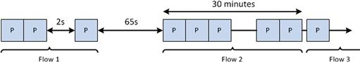
When a new packet is analyzed and contains the same 5-tuple attribute values, then that data is appended to the flow record that already exists. Data will be appended to this flow record for as long as packets matching the 5-tuple attribute values are observed. There are three conditions in which a flow record might be terminated (Figure 4.2):
1. Natural Timeout: Whenever communication naturally ends based upon the specification of the protocol. This is tracked for connection-oriented protocols, and will look for things like RST packets or FIN sequences in TCP.
2. Idle Timeout: When no data for a flow has been received within thirty seconds of the last packet, the flow record is terminated. Any new packets with the same 5-tuple attribute values after this thirty seconds has elapsed will result in the generation of a new flow record. This value is configurable.
3. Active Timeout: When a flow has been open for thirty minutes, the flow record is terminated and a new one is created with the same 5-tuple attribute values. This value is configurable.
Whenever packets are observed with new 5-tuple attribute values, a new flow record is created. There can be a large number of individual flow records open at any time.
I like to visualize this by imagining a man sitting on an assembly line. The man examines every packet that crosses in front of him. When he sees a packet with a unique set of 5-tuple attribute values, he writes those values on a can, collects the data he wants from the packet and places it into the can, and sits it to the side. Whenever a packet crosses the assembly line with values that match what is written on this can, he throws the data he wants from the packet into the can that is already sitting there. Whenever one of the three conditions for flow termination listed above are met, he puts a lid on the can, and sends it away.
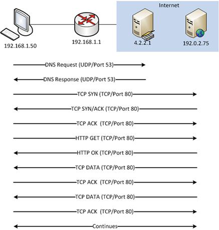
As you might expect based upon this description, flows are generated in a unidirectional manner in most cases (some tools, such as YAF, can generate bidirectional flows). For instance, with unidirectional flows, TCP communication between 192.168.1.1 and 172.16.16.1 would typically spawn at least two flow records, one record for traffic from 192.168.1.1 to 172.16.16.1, and another for traffic from 172.16.16.1 to 192.168.1.1 (Table 4.1).
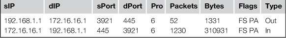
A more realistic scenario might be to imagine a scenario where a workstation (192.168.1.50) is attempting to browse a web page on a remote server (192.0.2.75). This communication sequence is depicted in Figure 4.3.
In this sequence, the client workstation (192.168.1.50) must first query a DNS server (4.2.2.1) located outside of his local network segment. Once a DNS response is received, the workstation can communicate with the web server. The flow records generated from this (as seen by the client workstation) would look like Table 4.2:

A good practice to help wrap your mind around flow data is to compare flow records and packet data for the same time interval. Viewing the two data types and their representations of the same communication side-by-side will help you to learn exactly how flow data is derived. Next, we will look at a few of the major flow types.
NetFlow
NetFlow was originally developed by Cisco in 1990 for use in streamlining routing processes on their network devices. In the initial specification, a flow record was generated when the router identified the first packet in new network conversations. This helped baseline network conversations and provided references for the router to compare to other devices and services on the network. These records were also used to identify and summarize larger amounts of traffic to simplify many processes, such as ACL comparisons. They also had the added benefit of being more easily parseable by technicians. Twenty-three years later, we have seen advancement of this specification through nine versions of NetFlow, including several derivative works. The features of these versions vary greatly and are used differently by individuals in various job functions, from infrastructure support and application development to security.
NetFlow v5 and v9
The two most commonly used NetFlow standards are V5 and V9. NetFlow V5 is by far the most accessible NetFlow solution because most modern routing equipment supports NetFlow V5 export. NetFlow V5 flow records offer standard 5-tuple information as well all of the necessary statistics to define the flow aggregation of the packets being summarized. These statistics allow analysis engines to streamline the parsing of this information. Unlike NetFlow V9 and IPFIX, NetFlow V5 does not support the IPV6 protocol, which may limit its ability to be used in certain environments.
NetFlow V9 is everything V5 is, but so much more. NetFlow V9 provides a new template that offers quite a bit more detail in its logging. Whereas NetFlow V5 offers 20 data fields (two of those are padding), NetFlow V9 has 104 field type definitions. These modified field types can be sent via a templated output to comprise the configurable record. Thus, an administrator can use NetFlow V9 to generate records that resemble V5 records by configuring these templates. NetFlow V9 also provides IPV6 support. If you’d like to know more about the differences in NetFlow V5 and V9, consult Cisco’s documentation.
Mike Patterson of Plixer provides one of the best and most entertaining examples on the comparison of NetFlow V5 and NetFlow V9 in a three-part blog at Plixer.com.1 He states that the lack of V9 usage is almost entirely due to a lack of demand for the increased utility that V9 can offer. Mike argues that NetFlow V5 is like a generic hamburger. It will fulfill your needs, but generally do nothing more. However, depending on your situation, you might only desire sustenance. In that case, a generic hamburger is all you need. The generic hamburger is an easy and cheap way to satisfy hunger, providing only the bare minimum in features, but it is everything you need. NetFlow V9 on the other hand, is an Angus cheeseburger with all the trimmings. Most administrators either have minimal requirements from NetFlow data and don’t require the extra trimmings that NetFlow V9 offers, or they don’t have a method of interacting with the data as they did with NetFlow V5. Both of these reasons account for a lack of NetFlow V9 adoption.
IPFIX
IPFIX has a lot in common with NetFlow V9 as it is built upon the same format. IPFIX is a template-based, record-oriented, binary export format.2 The basic unit of data transfer in IPFIX is the message. A message contains a header and one or more sets, which contain records. A set may be either a template set or a data set. A data set references the template describing the data records within that set. IPFIX falls into a similar area as NetFlow V9 when it comes to adoption rate. The differences between NetFlow V9 and IPFIX are functional. For instance, IPFIX offers variable length fields to export custom information, where NetFlow V9 does not. It also has a scheme for exporting lists of formatted data. There are a number of differences between NetFlow V9 and IPFIX, but one word really defines them; IPFIX is “flexible”. I use this word specifically because the extension to NetFlow V9 that makes it very similar to IPFIX is call “Flexible NetFlow”, but that version falls out of the scope of this book.
Other Flow Types
Other flow technologies exist that could already be in use within your environment, but the question of accessibility and analysis might make them difficult to implement in a manner that is useful for NSM purposes. Juniper devices may offer Jflow while Citrix has AppFlow. One of the more common alternatives to NetFlow and IPFIX is sFlow, which uses flow sampling to reduce CPU overhead by only taking representative samplings of data across the wire. Variations of sFlow are becoming popular with vendors, with sFlow itself being integrated into multiple networking devices and hardware solutions. These other flow types leverage their own unique traits, but also consider that while you might have an accessible flow generator, be sure you have a means of collecting and parsing that flow data to make it an actionable data type.
In this book, we try our best to remain flow type agnostic. That is to say that when we talk about the analysis of flow data, it will be mostly focused on the standard 5-tuple that is included in all types of flow data.
Collecting Session Data
Session data can be collected in a number of different ways. Regardless of the method being used, a flow generator and collector will be required. A flow generator is the hardware or software component that creates the flow records. This can be done from either the parsing of other data, or by collecting network data directly from a network interface. A flow collector is software that receives flow records from the generator, and stores them in a retrievable format.
Those who are already performing FPC data collection will often choose to generate flow records from this FPC data. However, in most cases, the FPC data you are collecting will be filtered, which means you will be unable to generate flow records for the network traffic that isn’t captured. Furthermore, if there is packet loss during your FPC capture, you will also lose valuable flow data. While this type of filtering is useful for maximizing disk utilization when capturing FPC data, the flow records associated with this traffic should be retained. This method of flow data generation isn’t usually recommended.
The preferred method for session data generation is to capture it directly off of the wire in the same manner that FPC data or NIDS alert data might be generated. This can either be done by software on a server, or by a network device,like a router. For the purposes of this chapter, we will categorize generation by devices as “hardware generation” and generation by software as “software generation”.
Hardware Generation
In many scenarios, you will find that you already have the capability to generate some version of flow data by leveraging existing hardware. In these situations, you can simply configure a flow-enabled router with the network address of a destination collector and flow records from the router’s interface will be sent to that destination.
While hardware collection may sound like a no-brainer, don’t be surprised when your network administrator denies your request. On routing devices that are already being taxed by significant amounts of traffic, the additional processing required to generate and transmit flow records to an external collector can increase CPU utilization to the point of jeopardizing network bandwidth. While the processing overhead from flow generation is minimal, this can cause a significant impact in high traffic environments.
As you might expect, most Cisco devices inherently have the ability to generate NetFlow data. In order to configure NetFlow generation on a Cisco router, consult with the appropriate Cisco reference material. Cisco provides guides specifically for configuring NetFlow with Cisco IOS, which can be found here: http://www.cisco.com/en/US/docs/ios/netflow/command/reference/nf_cr_book.pdf.
Software Generation
The majority of NSM practitioners rely on software generation. The use of software for flow generation has several distinct advantages, the best of which is the flexibility of the software deployment. It is much easier to deploy a server running flow generation software in a network segment than to re-architect that segment to place a flow generating router. Generating flow data with software involves executing a daemon on your sensor that collects and forwards flow records based upon a specific configuration. This flow data is generated from the data traversing the collection interface. In most configurations, this will be the same interface that other collection and detection software uses.
Now, we will examine some of the more common software generation solutions.
Fprobe
Fprobe is an example of a minimalist NetFlow generation solution. Fprobe is available in most modern Linux distribution repositories and can be installed on a sensor easily via most package management systems, such as yum or apt.
If outside network connections are not available at your sensor location, the package can be compiled and installed manually with no odd caveats or obscure options. Once installed, Fprobe is initiated by issuing the fprobe command along with the network location and port where you are directing the flow data. As an example, if you wanted to generate flow data on the interface eth1, and send it to the collector listening on the host 192.168.1.15 at port 2888, you would issue the following command:
fprobe -i eth1 192.168.1.15:2888
YAF
YAF (Yet Another Flowmeter) is a flow generation tool that offers IPFIX output. YAF was created by the CERT Network Situation Awareness (NetSA) team, who designed it for generating IPFIX records for use with SiLK (which will be discussed this later in this chapter).
As mentioned before, NetFlow v5 provides unidirectional flow information. This can result in redundant data in flow statistics that, on large distributed flow collection systems, can substantially affect data queries. To keep up with naturally increasing bandwidth and to provide bidirectional flow information for analysts, IPFIX was deemed to be a critical addition to SiLK, and YAF was created as an IPFIX generator. A bonus to using YAF is the ability to use the IPFIX template architecture with SiLK application labels for more refined analysis that you cannot get through the NetFlow V5 5-tuple.
Depending on your goals and the extent of your deployment, YAF might be a necessity in your IDS environment. If so, installing YAF is fairly straightforward. This book won’t go into detail on this process, but there are a few details that can help streamline the process. Before compiling YAF, please make sure to review the NetSA documentation thoroughly. NetSA also has supplementary install tutorials that will take you through the installation and initialization of YAF. This documentation can be found here: https://tools.netsa.cert.org/confluence/pages/viewpage.action?pageId=23298051.
Collecting and Analyzing Flow Data with SiLK
SiLK (System for Internet-Level Knowledge) is a toolset that allows for efficient manageable security analysis across networks. SiLK serves as a flow collector, and is also an easy way to quickly store, access, parse, and display flow data. SiLK is a project currently developed by the CERT NetSA group, but like most great security tools, it was the result of necessity being the mother of invention. Originally dubbed “Suresh’s Work”, SiLK was the result of an analyst needing to parse flow in a timely and efficient way, without the need for complex CPU intensive scripts. SiLK is a collection of C, Python, and Perl, and as such, works in almost any UNIX-based environment.
The importance of documentation is paramount. No matter how great of a tool, script, or device you create, it is nothing if it can only be used by the developer. The documentation for SiLK is second to none when it comes to truly helpful reference guides for an information security tool. To emphasize the importance of this documentation, the following sections will use this guide as both reference, and as part of a basic scenario in how to use SiLK.3 It is not an overstatement to suggest that the SiLK documentation and the community that supports the tool are easily some of the best features of the SiLK project.
SiLK Packing Toolset
The SiLK toolset operates via two components: the packing system and the analysis suite. The packing system is the method by which SiLK collects and stores flow data in a consistent, native format. The term “packing” refers to SiLK’s ability to compress the flow data into a space-efficient binary format ideal for parsing via SiLK’s analysis suite. The analysis suite is a collection of tools intended to filter, display, sort, count, group, mate, and more. The analysis tool suite is a collection of command line tools that provide an infinite level of flexibility. While each tool itself is incredibly powerful, each tool can also be chained together with other tools via pipes based on the logical output of the previous tool.
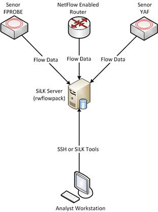
In order to utilize SiLK’s collection and analysis features, you must get data to it from a flow generator. When the collector receives flow records from a generator, the records are logically separated out by flow type. Flow types are parsed based upon a configuration file that determines if the records are external-to-internal, internal-to-external, or internal-to-internal in relation to the network architecture.
In SiLK, the listening collection process is a tool known as rwflowpack. Rwflowpack is in charge of parsing the flow type, determining what sensor the data is coming from, and placing the refined flow data into its database for parsing by any of the tools within the analysis toolset. This workflow is shown in Figure 4.4.
The execution of Rwflowpack is governed by a file named rwflowpack.conf, as well as optional command line arguments that can be issued during execution. The most common method to initiate rwflowpack is the command:
service rwflowpack start
Rwflowpack will confirm that the settings in the silk.conf and sensor.conf files are configured correctly and that all listening sockets identified by sensor.conf are available. If everything checks out, Rwflowpack will initialize and you will receive verification on screen.
While the packing process in SiLK is straightforward, it has more options that can be utilized outside of just receiving and optimizing flow data. The SiLK packing system has eight different tools used to accept and legitimize incoming flows. As previously mentioned, rwflowpack is a tool used to accept flow data from flow generators defined by SiLK’s two primary configuration files, silk.conf and sensor.conf, and then convert and sort the data into specific binary files suitable for SiLK’s analysis suite to parse. Forwarding flow data directly to an rwflowpack listener is the least complicated method of generating SiLK session data. Often the need arises for an intermediary to temporarily store and forward data between the generator and collector. For this, flowcap can be utilized. In most cases, flowcap can be considered a preprocessor to rwflowpack in that it first takes the flow data and sorts it into appropriate bins based on flow source and a unit or time variable. The SiLK documentation describes this as storing the data in “one file per source per quantum,” with a quantum being either a timeout or a maximum file size. The packing system also has a number of postprocessing abilities with tools such as rwflowappend, rwpackchecker, and rwpollexec. Rwflowappend and Rwpackchecker do exactly what they say; rwflowappend will append SiLK records to existing records and rwpackchecker checks for data integrity and SiLK file corruptions. Rwpollexec will monitor the incoming SiLK data files and run a user-specified command against each one. Rwflowappend, rwpackchecker and rwpollexec can be referred to as postprocessors because they further massage the SiLK data after rwflowpack has converted the raw flows into binary SiLK files. The moral of this story is that there are more than enough ways to get your data to rwflowpack for conversion into SiLK binary files.
SiLK Flow Types
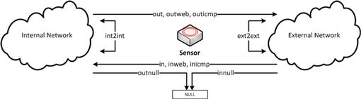
SiLK organizes flows into one of several types that can be used for filtering and sorting flow records. This is handled based upon the network ranges provided for internal and external ipblocks in the sensor.conf configuration file used by rwflowpack (Figure 4.5). These flow types are:
• In: Inbound to a device on an internal network
• Out: Outbound to a device on an external network
• Int2int: From an internal network to the same, or another internal network
• Ext2ext: From an external network to the same, or another external network
• Inweb: Inbound to a device on an internal network using either port 80, 443, or 8080.
• Outweb: Outbound to a device on an external network using either port 80, 443, or 8080.
• Inicmp: Inbound to a device on an internal network using ICMP (IP Protocol 1)
• Outicmp: Outbound to a device on an external network using ICMP (IP Protocol 1)
• Innull: Inbound filtered traffic or inbound traffic to null-ipblocks specified in sensor.conf
• Outnull: Outbound filtered traffic or outbound traffic to null-ipblocks specified in sensor.conf
• Other: Source not internal or external, or destination not internal or external
Understanding these flow types will be helpful when using some of the filtering tools we will talk about next.
SiLK Analysis Toolset
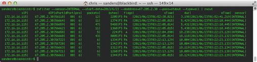
The analysis toolset is where you will spend the majority of your time when working with flow data. There are over 55 tools included in the SiLK installation, all of which are useful, with some being used more frequently. These analysis tools are meant to work as a cohesive unit, with the ability to pipe data from one tool to another seamlessly. The most commonly used tool in the suite is rwfilter. Rwfilter takes the SiLK binary files and filters through them to provide only the specific data that the analyst requires. We’ve spoken at length about how the size of flow records allow you to store them for a significant time, so it becomes clear that there must be a convenient way to apply filters to this data in order to only see data that is relevant given your specific task. For instance, an analyst might only want to examine a week of data from a year ago, with only source IP addresses from a particular subnet, with all destination addresses existing in a specific country. Rwfilter makes that quick and easy. The output of rwfilter, unless specified, will be another SiLK binary file that can continue to be parsed or manipulated via pipes. The tool is very thoroughly covered in the SiLK documentation and covers categories for filtering, counting, grouping, and more. As this is the collection section of the book, we will only cover a few brief scenarios with the analysis toolset here.
Installing SiLK in Security Onion
In this book, we don’t go into the finer details of how to install each of these tools, as most of those processes are documented fairly well, and most of them come pre-installed on the Security Onion distribution if you want to test them. Unfortunately, at this time of this writing, SiLK doesn’t come preinstalled on Security Onion like all of the other tools in this book. As such, you can find detailed instructions on this installation process on the Applied NSM blog at: http://www.appliednsm.com/silk-on-security-onion/.
Filtering Flow Data with Rwfilter
The broad scope of flow collection and the speed of flow retrieval with SiLK makes a strong case for the inclusion of flow collection in any environment. With SiLK, virtually any analyst can focus the scope of a network incident with a speed unmatched by any other data type. The following scenarios present a series of common situations in which SiLK can be used to either resolve network incidents, or to filter down a large data set to a manageable size.
One of the first actions in most investigations is to examine the extent of the harassment perpetrated by an offending host with a single IP address. Narrowing this down from PCAP data can be extremely time consuming, if not impossible. With SiLK, this process can start by using the rwfilter command along with at least one input, output, and partitioning option. First is the --any-address option, which will query the data set for all flow records matching the identified IP address. This can be combined with the --start-date and --end-date options to narrow down the specific time frame we are concerned with. In addition to this, we will provide rwfilter with the –type = all options, which denotes that we want both inbound and outbound flows, and the --pass = stdout option, which allows us to pass the output to rwcut (via a pipe symbol) so that it can be displayed within the terminal window. This gives us an rwfilter command that looks like this:
rwfilter --any-address = 1.2.3.4 --start-date = 2013/06/22:11 --end-date = 2013/06/22:16 --type = all --pass = stdout | rwcut
Denoting only a start-date will limit your search to a specific quantum of time based on the smallest time value. For instance, --start-date = 2013/06/22:11 will display the entirety of the filter matched flow data for the 11th hour of that day. Similarly, if you have –start-date = 2013/06/22, you will receive the entire day’s records. The combination of these options will allow you to more accurately correlate events across data types and also give you 1000 ft visibility on the situation itself.
For example, let’s say that you have a number of events where a suspicious IP (6.6.6.6) is suddenly receiving significant encrypted data from a secure web server shortly after midnight. The easiest way to judge the extent of the suspicious traffic is to run the broad SiLK query:
rwfilter --start-date = 2013/06/22:00 --any-address = 6.6.6.6 --type = all --pass = stdout | rwcut
If the data is too expansive, simply add in the partitioning option “--aport = 443” to the previous filter to narrow the search to just the events related to the interactions between the suspicious IP and any secure web servers. The --aport command will filter based upon any port that matches the provided value, which in this case is port 443 (the port most commonly associated with HTTPS communication).
rwfilter --start-date = 2016/06/22:00 --any-address = 6.6.6.6 --aport = 443 --type = all --pass = stdout | rwcut
After looking at that data, you might notice that the offending web server is communicating with several hosts on your network, but you want to zero in on the communication occurring from one specific internal host (192.168.1.100) to the suspicious IP. In that case, instead of using the --any-address option, we can use the --saddress and --daddress options, which allow you to filter on a particular source and destination address, respectively. This command would look like:
rwfilter --start-date = 2013/06/22:00 --saddress = 192.168.1.100 --daddress = 6.6.6.6 --aport = 443 --type = all --pass = stdout | rwcut
Piping Data Between Rwtools
An analyst often diagnoses the integrity of the NSM data by evaluating the health of incoming traffic. This example will introduce a number of rwtools and the fundamentals of piping data from one rwtool to another.
It is important to understand that rwfilter strictly manipulates and narrows down data fed to it from binary files and reproduces other binary files based on those filter options. In previous examples we have included the --pass = stdout option to send the binary data which matches a filter to the terminal output. We piped this binary data to rwcut in order to convert it to human readable ASCII data in the terminal window. In this sense, we have already been piping data between rwtools. However, rwcut is the most basic rwtool, and the most essential because it is almost always used to translate data to an analyst in a readable form. It doesn’t do calculations or sorting, it simply converts binary data into ASCII data and manipulates it for display at the user’s discretion through additional rwcut options.
In order to perform calculations on the filtered data, you must pipe directly from the filtered data to an analysis rwtool. For this example, we’ll evaluate rwcount, a tool used to summarize total network traffic over time. Analyzing the total amount of data that SiLK is receiving can provide an analyst with a better understanding of the networks that he/she is monitoring. Rwcount is commonly used for the initial inspection of new sensors. When a new sensor is brought online, it comes with many caveats. How many end users are you monitoring? When is traffic the busiest? What should you expect during late hours? Simply getting a summary of network traffic is what rwcount does. Rwcount works off of binary SiLK data. This means that piping data to it from rwfilter will give you an ASCII summary of any data matching your filter.
Consider a scenario where you want to evaluate how much data is being collected by your SiLK manager. We’ll use rwfilter to output all of the data collected for an entire day, and we will pipe that data to rwcount:
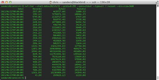
rwfilter --start-date = 2013/6/22 --proto = 0-255 --pass = stdout --type = all | rwcount --bin-size = 60
This command will produce a summary of traffic over time in reference to total records, bytes, and packets per minute that match the single day filter described. This time interval is based upon the --bin-size option, which we set to 60 seconds. If you increase the bin size to 3600, you will get units per hour, which is shown in Figure 4.6. As mentioned before, rwfilter requires, at minimum, an input switch, a partitioning option, and an output switch. In this case, we want the input switch to identify all traffic (--type = all) occurring on 2013/6/22. In order to pass all data, we will specify that data matching all protocols (--proto = 0-255) should pass to stdout (--pass = stdout). This will give us all of the traffic for this time period.
You’ve now seen basic scenarios involving filtering flow records using rwfilter, and the use of rwcount, a tool that is of great use in profiling your networks at a high level. We’ll now combine these two tools and add another rwtool called rwsetbuild. Rwsetbuild will allow you to build a binary file for SiLK to process using various partitioning options. Quite often, you’ll find you need a query that will consider multiple IP addresses. While there are tools within SiLK to combine multiple queries, rwsetbuild makes this unnecessary as it will streamline the process by allowing you to generate a flat text list of IP addresses and/or subnets (we’ll call it testIPlist.txt), and run them through rwsetbuild with the following command:
rwsetbuild testIPlist.txt testIPlist.set
Having done this, you can use the --anyset partitioning option with rwfilter to filter flow records where any of the IP addresses within the list appear in either source or destination address fields. The command would look like:
rwfilter --start-date = 2014/06/22 --anyset =/home/user/testIPlist.set --type = all --pass = stdout | rwcut
This ability can be leveraged to gather a trove of useful information. Imagine you have a list of malicious IP addresses that you’re asked to compare with communication records for your internal networks. Of particular interest is how much data has been leaving the network and going to these “bad” IP addresses. Flow data is the best option for this, as you can couple what you’ve learned with rwsetbuild and rwcount to generate a quick statistic of outbound data to these malicious devices. The following process would quickly yield a summary of outbound data per hour:
1. Add IP addresses to a file called badhosts.txt.
2. Create the set file with the command:
rwsetbuild badhosts.txt badhosts.set
3. Perform the query and create the statistic with the command:
rwfilter --start-date = 2013/06/22 --dipset = badhosts.set --type = all --pass = stdout | rwcount --bin-size = 3600
The next scenario is one that I run into every day, and one that people often ask about. This is a query for “top talkers”, which are the hosts on the network that are communicating the most.
Top talker requests can have any number of variables involved as well, be it top-talkers outbound to a foreign country, top talking tor exit nodes inbound to local devices, or top talking local devices on ports 1-1024. In order to accomplish tasks such as these, we are interested in pulling summary statistics that match given filters for the data we want. If you haven’t already guessed it, the tool we’re going to use is creatively named rwstats. Piping rwfilter to rwstats will give Top-N or Bottom-N calculations based on the results of the given filter. In this example, we’ll analyze the most active outbound connections to China. Specifically, we’ll look at communications that are returning data on ephemeral ports (> 1024). This can be accomplished with the following command:
rwfilter --start-date = 2013/06/22 --dcc = cn --sport = 1024-65535 --type = all --pass = stdout | rwstats --top --count = 20 --fields = sip --value = bytes
You will note that this rwfilter command uses an option we haven’t discussed before, --dcc. This option can be used to specify that we want to filter based upon traffic to a particular destination country code. Likewise, we could also use the command --scc to filter based upon a particular source country. The ability to filter data based upon country code doesn’t work with an out-of-the-box SiLK installation. In order to utilize this functionality and execute the command listed above, you will have to complete the following steps:
1. Download the MaxMind GeoIP database with wget:
wget http://geolite.maxmind.com/download/geoip/database/GeoLiteCountry/GeoIP.dat.gz
2. Unzip the file and convert it into the appropriate format:
gzip -d -c GeoIP.dat.gz | rwgeoip2ccmap --encoded-input > country_codes.pmap
3. Copy the resulting file into the appropriate location:
cp country_codes.pmap /usr/local/share/silk/
The results of this query take the form shown in Figure 4.7.
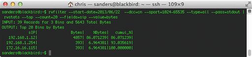
In this example, rwstats only displays three addresses talking out to China, despite the --count = 20 option on rwstats that should show the top twenty IP addresses. This implies that there are only three total local IP addresses talking out to China in the given time interval. Had there been fifty addresses, you would have only seen the top 20 local IP addresses. The --bytes option specifies that the statistic should be generated based upon the number of bytes of traffic in the communication. Leaving off the –value option will default to displaying the statistic for total number of outbound flow records instead.
The next logical step in this scenario would be to find out who all of these addresses are talking to, and if it accepts the traffic. Narrowing down the results by augmenting the rwfilter portion of the command in conjunction with altering the fields in rwstats will provide you with the actual Chinese addresses that are being communicated with. We’ve also used the --saddress option to narrow this query down to only the traffic from the host who is exchanging the most traffic with China.
rwfilter --start-date = 2013/06/22 --saddress = 192.168.1.12 --dcc = cn --sport = 1024-65535 --type = all --pass = stdout | rwstats --top --count = 20 --fields = dip --value = bytes
Finally, utilizing the rwfilter commands in previous scenarios, you can retrieve the flow records for each host in order to gauge the type of data that is being transferred. You can these use this information, along with the appropriate timestamps, to retrieve other useful forms of data that might aid in the investigation, such as PCAP data.
Other SiLK Resources
SiLK and YAF are only a small portion of the toolset that NetSA offers. I highly recommend that you check out the other public offerings that can work alongside SiLK. NetSA offers a supplementary tool to bring SiLK to the less unix-savvy with iSiLK, a graphical front-end for SiLK. Another excellent tool is the Analysis Pipeline, an actively developed flow analysis automation engine that can sit inline with flow collection. Once it has been made active with an appropriate rule configuration, the Analysis Pipeline can streamline blacklist, DDOS, and beacon detection from SiLK data so that you don’t need to script these tools manually.
While the documentation is an excellent user reference for SiLK and is an invaluable resource for regular analysts, SiLK also has complementary handbooks and guides to help ignite the interests of amateur session data analysts or assist in generating queries for the seasoned professional. The ‘Analyst Handbook’ is a comprehensive 107 page guide to many SiLK use cases.4 This handbook serves as the official tutorial introduction into using SiLK for active analysis of flow data. Other reference documents pertain to analysis tips and tricks, installation information, and a full PySiLK starter guide for those wanting to implement SiLK as an extension to python. We highly recommended perusing the common installation scenarios to get a good idea of how you will be implementing SiLK within your environment.
Collecting and Analyzing Flow Data with Argus
While Applied NSM will focus on SiLK as the flow analysis engine of choice, we would be remiss if we didn’t at least mention Argus. Argus is a tool that also happens to be the product of some of CERT-CC’s early endeavors in the field of flow analysis. Argus first went into government use in 1989, becoming the world’s first real-time network flow analyzer.5 Starting in 1991, CERT began officially supporting Argus. From there, Argus saw rapid development until 1995 when it was released to the public.
Argus defines itself as a definitive flow solution that encompasses more than just flow data, but instead provides a comprehensive systematic view of all network traffic in real time. Argus is a bi-directional flow analysis suite that tracks both sides of network conversations and reports metrics for the same flow record.6 While offering many of the same features as other IPFIX flow analysis solutions, Argus has its own statistical analysis tools and detection/alerting mechanisms that attempt to separate it from other solutions. In the next few sections, I’ll provide an overview of the basic solution architecture and how it is integrated within Security Onion. In doing so, I won’t rehash a lot of concepts I’ve already covered, but instead, will focus on only the essentials to make sure you can capture and display data appropriately. As mentioned before, Argus sets itself apart in a few key ways, so I’ll provide examples where these features might benefit your organization more than the competing flow analysis engines.
Solution Architecture
Even though Argus comes packaged within Security Onion, it is important to understand the general workflow behind obtaining and verifying the data. Even with Security Onion, you might find yourself troubleshooting NSM collection issues, or you might desire to bring in data from external devices that aren’t deployed as Security Onion sensors. In these events, this section should give you an understanding of the deployment of Argus and how its parts work together to give you a flow analysis package with little overhead.
We are going to frame this discussion with Argus as a standalone rollout. Argus consists of two main packages. This first package is simply known as the generic “Argus” package, which will record traffic seen at a given network interface on any device. That package can then either write the data to disk for intermittent transfer or maintain a socketed connection to the central security server for constant live transfer. This is the component that will typically reside on a sensor, and will transmit data back to a centralized logging server.
The second Argus package is referred to as the Argus Client package. This package, once deployed correctly, will read from log files, directories, or a constant socket connection for real-time analysis. These client tools do more than collect data from the external generator; they will serve as the main analysis tools for the duration of your Argus use. With that said, you will need the client tools on any device that you do Argus flow analysis from.
There isn’t much difference in the workflow of Argus and other flow utilities. The basic idea is that a collection interface exists that has a flow-generating daemon on it. That daemon sees the traffic, generates flows, and forwards the flow data to a central collection platform where storage and analysis of that data can occur.
Features
Argus is unique because it likely has more features built into it than most other flow analysis tools. A standalone deployment of Argus can do more than basic flow queries and statistics. Since partial application data can be retrieved with the collection of IPFIX flow data imported into Argus, it can be used to perform tasks such as filtering data based upon HTTP URLs. I mention that Argus is powerful by itself, because in today’s NSM devices we generally have other tools to perform these additional tasks. This makes mechanisms like URL filtering redundant if it is working on top of other data types such as packet string data. Since we are referring to the basic installation of Argus within Security Onion, I will not be discussing the additional Argus application layer analysis. In Chapter 6 we will be talking about packet string data and how it can perform those tasks for you.
Basic Data Retrieval
Data retrieval in different flow analysis tools can result in a déjà vu feeling due to the similarity in the data ingested by the tools. Ultimately, it is the query syntax and statistic creation abilities of these tools that differ. Argus has what appears to be a basic querying syntax on initial glance; however, the learning curve for Argus can be steep. Given the large number of query options and the vague documentation available for the tool online, the man pages for the tools will be your saving grace when tackling this learning curve.
The most useful tool within the Argus Client suite of tools is ra. This tool will provide you with the initial means to filter and browse raw data collected by Argus. Ra must be able to access a data set in order to function. This data can be provided through an Argus file from the –r option, from piped standard input, or from a remote feed. Since we are working so intimately with Security Onion, you can reference the storage directory for Argus files in /nsm/sensor_data/< interface >/argus/. At first glance, ra is a simple tool, and for the most part, you’ll probably find yourself making basic queries using only a read option with a Berkeley Packet Filter (BPF) at the end. For example, you might have a suspicion that you have several geniuses on your network due to HTTP logs revealing visits to www.appliednsm.com. One way to view this data with Argus would be to run the command:
ra –r /nsm/sensor_data/< interface >/argus/< file > - port 80 and host 67.205.2.30
Sample output from this command is shown below in Figure 4.8.
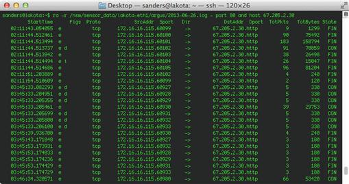
The nicest benefit of Argus over competing flow analysis platforms is its ability to parse logs using the same BPFs that tools like Tcpdump use. This allows for quick and effective use of the simplest functions of ra and Argus. After understanding the basic filter methodology for ra, you can advance the use of ra with additional options. As I stated before, ra can process standard input and feed other tools via standard output. In doing so, you can feed the data to other Argus tools. By default, ra will read from standard-in if the –r option is not present. Outputting ra results to a file can be done with the –w option. Using these concepts, we could create the following command:
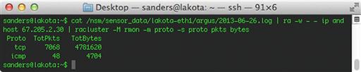
cat /nsm/sensor_data/< interface >/argus/< file > | ra -w - - ip and host 67.205.2.30 | racluster -M rmon -m proto –s proto pkts bytes
This example will use ra to process raw standard input and send the output to standard out via the -w option. This output is then piped to the racluster tool. Racluster performs ra data aggregation for IP profiling. In the example, racluster is taking the result of the previous ra command and aggregating the results by protocol. A look at the manual page for ra reveals that it also accepts racluster options for parsing the output. The example command shown above would produce an output similar to what is shown in Figure 4.9.
Other Argus Resources
Though this book won't cover the extensive use of Argus from an analysis standpoint, it is still worth reviewing in comparison to other flow analysis suites like SiLK. When choosing a flow analysis tool each analyst must identify which tool best suits his/her existing skill set and environment. The ability to use BPFs in filtering data with ra makes Argus immediately comfortable to even the newest flow analysts. However, advanced analysis with Argus will require extensive parsing skills and a good understanding of the depth of ratools to be successful. If you want to learn more about Argus, you can visit http://qosient.com/argus/index.shtml, or for greater technical detail on how to work with Argus, go to http://nsmwiki.org/index.php?title=Argus.
Session Data Storage Considerations
Session data is miniscule in size compared to other data types. However, flow data storage cannot be an afterthought. I’ve seen situations where a group will set up flow as their only means of network log correlation, only to realize that after a month of data collection, they can’t query their logs anymore. This results from improper flow rollover. Flow data can gradually increase in size to an unmanageable level if left unchecked. There is no specific recommendation on the amount of storage you’ll need for flow data, as it depends on the data that is important to you, and how much throughput you have. With that said, just because are able to define a universal filter for all traffic you are collecting doesn’t mean you should. Even though you might not be collecting FPC data for certain protocols, such as encrypted GRE tunnels or HTTPS traffic, you should still keep flow records of these communications.
To estimate the amount of storage space needed for flow data, the CERT NetSA team provides a SiLK provisioning worksheet that can help. It can be found at: http://tools.netsa.cert.org/releases/SiLK-Provisioning-v3.3.xlsx.
There are many ways to manage your network log records, but I find one of the simplest and easiest to maintain is a simple cron job that watches all of your data and does rollover as necessary or based upon a time interval. Many of your data capture tools will feature rollover features in the process of generating the data; however, you’ll likely have to manage this rollover manually. This can be the case with flow data, though many organizations opt to only roll over flow data when required. One solution to limit the data is to simply create a cron job that cleans the flow data directory by purging files that are older that X days. One SiLK specific example of a cron job that will do this is:
30 12 * * * find /data/silk/* -mtime + 29 -exec rm {} ;
In this example, the /data/silk/ directory will be purged of all data files 30 days or older. This purge will occur every day at 12:30 PM. However, be careful to make sure that you’re not removing your configuration files if they are stored in the same directory as your data. Many organizations will also like to keep redundant storage of flow data. In that case, the following will move your data to a mounted external USB storage device.
*/30 * * * * rsync --update -vr /data/silk/ /mnt/usb/data/silk/ &> /dev/null
This command will copy all new flow files every 2 minutes. The method used to implement this cron job will vary depending on which operating system flavor you are using. In this spirit, it should be noted that SiLK also includes features to repeat data to other sites.
I like to include control commands like these in a general “watchdog” script that ensures services are restarted in the event of the occasional service failure or system reboot. In this watchdog script, I also include the periodic updating or removal of data, the transfer and copying of redundant data, status scripts that monitor sensor health, and the service health scripts that make sure processes stay alive. This has the added benefit of eliminating errors upon sensor startup, as the services in question will begin one the cron job starts rather than with all other kernel startup processes.
Ultimately, the greatest benefit of a centralized watchdog script is that it will provide a central point of reference for safely monitoring the health of your sensors, which includes ensuring that data is constantly flowing. The script below can be used to monitor YAF to make sure it is constantly running. Keep in mind that the script may require slight modifications to work correctly in your production environment.
#!/bin/bash
function SiLKSTART {
sudo nohup /usr/local/bin/yaf --silk --ipfix = tcp --live = pcap --out = 192.168.1.10 --ipfix-port = 18001 --in = eth1 --applabel --max-payload = 384 --verbose --log =/var/log/yaf.log &
}
function watchdog {
pidyaf = $(pidof yaf)
if [ -z “$pidyaf” ]; then
echo “YAF is not running.”
SiLKSTART
fi
}
watchdog
Rwflowpack is another tool that you may want to monitor to ensure that it is always running and collecting flow data. You can use the following code to monitor its status:
#!/bin/bash
pidrwflowpack = $(pidof rwflowpack)
if [ -z “$pidrwflowpack” ]; then
echo “rwflowpack is not running.”
sudo pidof rwflowpack | tr ' ' ' ' | xargs -i sudo kill -9 {}
sudo service rwflowpack restart
fi
Conclusion
In this chapter we provided an overview of the fundamental concepts associated with the collection of session data. This included an overview of different types of session data like NetFlow and IPFIX, as well as a detailed overview of data collection and retrieval with SiLK, and a brief overview of Argus. I can’t stress the importance of session data enough. If you are starting a new security program or beginning to develop an NSM capability within your organization, the collection of session data is the best place to start in order to get the most bang for your buck.
1http://www.plixer.com/blog/general/cisco-netflow-v5-vs-netflow-v9-which-most-satisfies-your-hunger-pangs/
2http://www.tik.ee.ethz.ch/file/de367bc6c7868d1dc76753ea917b5690/Inacio.pdf
3http://tools.netsa.cert.org/silk/docs.html
4http://tools.netsa.cert.org/silk/analysis-handbook.pdf
5http://www.qosient.com/argus/presentations/Argus.FloCon.2012.Tutorial.pdf