Packet Analysis
Abstract
The analysis phase of Network Security Monitoring is predicated on the analysis of data in order to determine if an incident has occurred. Since most of the data that is collected by NSM tools is related to network activity, it should come as no surprise that the ability to analyze and interpret packet data is one of the most important skills an analyst can have. In this first chapter of the analysis section of this book, we will dive into the world of packet analysis from the perspective of the NSM analyst. The main goal of this chapter is to equip you with the knowledge you need to understand packets at a fundamental level, while providing a framework for understanding the protocols that aren’t covered here. This chapter will use tcpdump and Wireshark to teach these concepts. At the end of the chapter, we will also look at a capture and display filters for packet analysis.
Keywords
Network Security Monitoring; Packets; Packet Analysis; Wireshark; tcpdump; filters; Berkeley Packet Filter; BPF; expressions; TCP; IP; UDP; ICMP; Header
Chapter Contents
Converting Hex to Binary and Decimal
Configuring Protocol Dissector Options
The analysis phase of Network Security Monitoring is predicated on the analysis of data to determine if an incident has occurred. Since most of the data that is collected by NSM tools is related to network activity, it should come as no surprise that the ability to analyze and interpret packet data is one of the most important skills an analyst can have. In this first chapter of the analysis section of this book, we will dive into the world of packet analysis from the perspective of the NSM analyst. This chapter will assume that the reader is somewhat familiar with how computers communicate over the network, but will assume no prior packet analysis knowledge. We will examine how to interpret packets using “packet math” and protocol header maps, and look at ways packet filtering can be performed. While discussing these topics we will use both tcpdump and Wireshark to interact with packets.
The main goal of this chapter is to equip you with the knowledge you need to understand packets at a fundamental level, while providing a framework for understanding the protocols that aren’t covered here.
Enter the Packet
The heterogeneous nature of computing is what allows a multitude of devices developed and manufactured by a variety of companies to interoperate with each other on a given network. Whether that network is a small network like the one in your house, a large network like a corporation might have, or a global network like the Internet, devices can communicate on it as long as they speak the right protocol.
A networking protocol is similar to a spoken or written language. A language has rules, such as how nouns must be positioned, how verbs should be conjugated, and even how individuals should formally begin and end conversations. Protocols work in a similar fashion, but instead of dictating how humans communicate, they dictate how network devices can communicate. Regardless of who manufactures a networking device, if it speaks TCP/IP, then it can most likely communicate with any other devices that speak TCP/IP. Of course, protocols come in a variety of forms, with some being more simple and others being more complex. Also, the combined efforts of multiple protocols are required for normal network communication to take place.
The evidence of a protocol in action is the packet that is created to conform to its standards. The term packet refers to a specially formatted unit of data that is transmitted across a network from one device to another. These packets are the building blocks of how computers communicate, and the purest essence of network security monitoring.
For a packet to be formed, it requires the combination of data from multiple protocols. For instance, a typical HTTP GET request actually requires the use of at least four protocols to ensure that the request gets from your web browser to a web server (HTTP, TCP, IP, and Ethernet). If you’ve looked at packets before, then you may have seen the packet displayed in a format similar to what is shown in Figure 13.1, where Wireshark is used to display information about the packets contents.

Wireshark is a great tool for interacting with and analyzing packets, but to really understand packets at a fundamental level, we are going to start with a much more fundamental tool, tcpdump (or its Windows alternative, Windump). While Wireshark is a great tool, it is GUI based and does a lot of the legwork for you in regards to packet dissection. On the other hand, tcpdump relies on you to do a lot of the interpretation for individual packets on your own. While this may seem a bit counterintuitive, it really challenges the analyst to think more about the packets they are seeing, and provides a fundamental understanding that can be better applied to any packet analysis tool, or even the raw parsing of packet data.
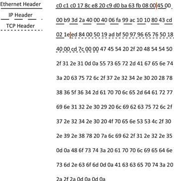
Now that we’ve seen Wireshark break down an HTTP GET Request packet, let’s look at the same packet in hexadecimal form. This output is achieved by using the command:
tcpdump –nnxr ansm-13-httpget.pcapng
We will discuss tcpdump later in this chapter, but for now, the packet is shown in Figure 13.2.

If you’ve never attempted to interpret a packet from raw hex before, then the output in Figure 13.2 can be a bit intimidating. However, it isn’t very hard to read this data if we break it down by protocol. We are going to do that, but first, let’s explore some basic packet math that will be necessary to proceed.
Packet Math
If you are anything like me, then the title of this section might get your blood boiling hotter than two dollar grits on the back burner of a twenty dollar stove. After all, there was no warning that math would be required! Don’t worry though, packet math is actually pretty easy, and if you can do basic addition and multiplication, then you should be fine.
Understanding Bytes in Hex
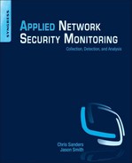
When examining packets at a lower level, such as with tcpdump, you will usually be looking at packet data represented in hexadecimal form. This hex format is derived from the binary representation of a byte. A byte is made up of 8 bits, which can either be a 1 or a 0. A single byte looks like this: 01000101.
To make this byte more readable, we can convert it to hex. This starts by splitting the byte into two halves, called nibbles (Figure 13.3). The first four bits is referred to as the higher order nibble, because it represents the larger valued portion of the byte. The second four bits is referred to as the lower order nibble, because it represents the lower valued portion of the byte.
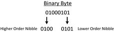
Each nibble of this byte is converted into a hex character to form a two character byte. For most beginners, the fastest way to calculate the hex value of a byte is to first calculate the decimal value of each nibble, shown in Figure 13.4.
While doing this calculation, notice that each position in the binary byte represents a value, and that this value increases from right to left, which is also how these positions are identified with the first position being the rightmost. The positions represent powers of 2, so the right most position is 20, followed by 21, 22, and 23. I find it easiest to use their decimal equivalents of 1, 2, 4, and 8 for performing calculations. With that said, if the position has a value of 1, then the value is added to a total. In the higher order nibble shown in Figure 13.4, there is only a value of 1 in the 3rd position, resulting in a total of 4. In the lower order nibble, there is a 1 in the 1st and 3rd positions, resulting in a total of 5 (1 + 4). The decimal values 4 and 5 represent this byte.
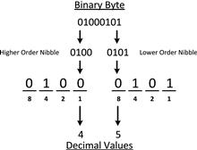
A hex character can range from 0-F, where 0-9 is equal to 0-9 in decimal, and A-F is equal to 10-15 in decimal. This means that 4 and 5 in decimal are equivalent to 4 and 5 in hexadecimal, meaning that 45 is the accurate hex representation of the byte 01000101. This entire process is shown in Figure 13.5.
Let’s try this one more time, but with a different byte. Figure 13.6 shows this example.

In this example, the higher order nibble has a 1 in the 2nd and 3rd position, resulting in a total of 6 (2 + 4). The lower order nibble has a 1 in the 2nd, 3rd, and 4th positions. This yields a decimal value of 14 (2 + 4 + 8). Converting these numbers to hex, 6 in decimal is equivalent to 6 in hex, and 14 in decimal is equivalent to E in hex. This means that 6E is the hex representation of 01101110.
Converting Hex to Binary and Decimal
We’ve discussed how to convert a binary number to hex, but later we will also need to know how to convert from hex values to decimal, so let’s approach that subject quickly. First, we will convert a hex number back into binary, and then into decimal. We will use the same example as earlier, and attempt to convert 0x6E to a decimal number.
As we now know, a two digit hex value represents a single byte, which is 8 bits. Each digit of the hex value represents a nibble of the byte. This means that 6 represents the higher order nibble of the byte and E represents the lower order nibble. First, we need to convert each of these hex digits back into their binary equivalent. The manner I like to use is to convert each digit into its decimal equivalent first. Remembering that hex is base 16, this means that 6 in hex is equivalent to 6 in decimal, and E is equivalent to 12 in decimal. Once we’ve determined those values, we can convert them to binary by placing 1’s in the appropriate bit positions (based on powers of 2) of each nibble. The result is a higher order nibble with the value 0100 and the lower order nibble of 1110.
Next, we can combine these nibbles to form a single byte, and consider each position as a power of 2 relative to the entire byte. Finally, we add up the values of the positions where the bit value is set to 1, yielding a decimal value of 110. This process is shown in Figure 13.7.

Counting Bytes
Now that you understand how to interpret bytes in hex, let’s talk about counting bytes. When examining packets at the hex level, you will spend a lot of time counting bytes. Although counting is pretty easy (no shame in using your fingers and toes!), there is an extra consideration when counting bytes in a packet.
As humans, we are used to counting starting from 1. When counting bytes, however, you must count starting from 0. This is because we are counting from an offset relative position.
To explain this, let’s consider the packet shown in in Figure 13.8.
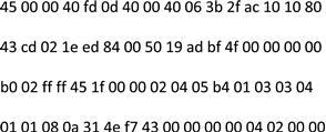
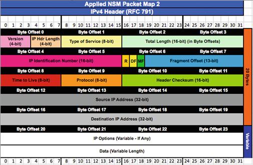
This figure shows a basic IP packet, spaced so that it is easier to read the individual bytes. In order to figure out what makes this packet tick, we might want to evaluate values in certain fields of this packet. The best way to do this is to “map” each field in the protocols contained within this packet. This book contains several protocol field maps in Appendix 3 that can be used to dissect fields within individual protocols. In this case, since we know this is an IP packet, let’s evaluate some of the values in the IP header. For convenience, it is shown in Figure 13.9:
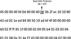
One useful piece of information that could help us dissect this packet further would be the embedded protocol that is riding on top of the IP header. The protocol map for IP indicates that this value is at byte 9. If you were to count bytes in this packet starting from 1, you would determine that the value of the embedded protocol field is 40, but this would be incorrect. When referring to a byte in this manner, it is actually referred to as byte offset 9, the ninth byte offset from 0, or more simply, 0x9. This means that we should be counting from 0, which shows that the true value of this field would be 06. This protocol value designates that TCP is the embedded protocol here. This is shown in Figure 13.10
Applying this knowledge to another field, the IP protocol map tells us that the Time-to-Live (TTL) field is in the eighth byte offset from 0. Counting from 0 at the beginning of the packet, you should see that the value for this field is 40, or 64 in decimal.
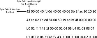
Looking at the protocol map, you will notice that some fields are less than a byte in size. For example, the 0x0 byte in this packet contains two fields: IP Version and IP Header Length. In this example, the IP Version field is only the higher order nibble of this byte, while the IP Header Length field is the lower order nibble of this byte. Referencing Figure 13.9, this means that the IP Version is 4. The IP header length is displayed as 5, but this field is actually a bit tricky. The IP header length field actually has a calculated value, and must be multiplied by four. In this case, we multiply the value 5 times 4, and end up at an IP header length of 20 bytes. With this knowledge, you ascertain that the maximum length of an IP header is 60 bytes, because the highest possible value in the IP header length field is F (15 in decimal), and 15 × 4 is 60 bytes. These fields are shown in Figure 13.11.
In a final example, you will notice that some fields span more than one byte. One such example of this is the source and destination IP address fields, which are each 4 bytes in length, and occur at positions 0×12 and 0×16 in the IP header, respectively. In our example packet, the source IP address breaks down as ac 10 10 80 (172.16.16.128 in decimal), and the destination IP address is 43 cd 02 1e (67.205.2.30 in decimal). This is shown in Figure 13.12
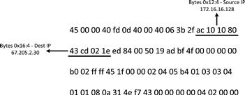
Take note of the special notation used in this figure to denote a field that is multiple bytes in length. When byte 0x16:4 is noted, this means to start at the sixteenth byte offset from 0, and then select four bytes from this point. This notation will come in handy later when we start writing packet filters.
At this point, we’ve looked at enough packet math to start dissecting packets at a low level. Hopefully it wasn’t too painful.
Dissecting Packets
With some math out of the way, let’s return to the packet shown in Figure 13.2 and break it down by each individual protocol. If you have an understanding of how packets are built, you know that a packet is built starting with the application layer data, and headers from protocols operating on lower layers are added as the packet is being built, moving from top to bottom. This means that the last protocol header that is added is at the Data Link layer, which means that we should encounter this header first. The most common data link layer protocol is Ethernet, but let’s verify that this is what’s being used here.
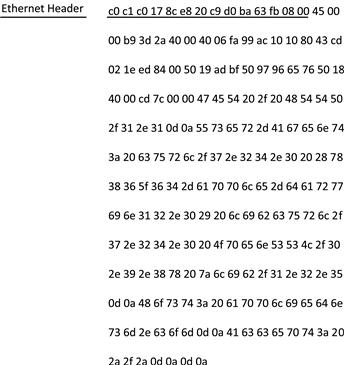
In order to verify that we are indeed seeing Ethernet traffic, we can compare what we know an Ethernet header should look like to what we have at the beginning of this packet. The Ethernet header format can be found in Appendix 3, but we’ve included it here in Figure 13.13 for convenience.

Looking at the Ethernet header format, you will see that the first 6 bytes of the packet are reserved for the destination MAC address, and the second six bytes, starting at 0x6, are reserved for the source MAC address. Figure 13.14 shows that these bytes do correspond to the MAC addresses of the two hosts in our example. The only other field that is included in the Ethernet header is the two-byte Type field at 0x12, which is used to tell us what protocol to expect after the Ethernet header. In this case, the type field has a hex value of 08 00, which means that the next embedded protocol that should be expected is IP. The length of the Ethernet header is static at 14 bytes, so we know that 00 is the last byte of the header.
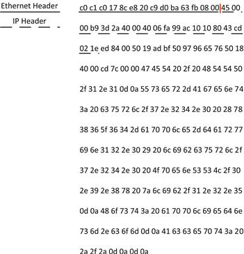
Since the Ethernet header was kind enough to tell us that we should expect an IP header next, we can apply what we know about the structure of the IP header to the next portion of the packet. We are attempting to break this packet down by individual protocol, so we aren’t concerned about every single value in this header, but there are a few values we will have to evaluate in order to determine the length of the IP header and what protocol to expect next.
First, we need to determine what version of IP is being used here. As we learned earlier, the IP version is identified by the higher order nibble of byte 0x0 in the IP header. In this case, we are dealing with IPv4.
The IP header is variable in length depending on a set of options it can support, so the next thing we need to ascertain is the length of the IP header. Earlier, we learned that the IP header length field is contained in the lower order nibble of byte 0×0 in the IP header, which has a value of 4. This is a computed field however, so we must multiply this field by 5 to arrive at the IP header length, which is 20 bytes. This means that the last two bytes of the IP header are 02 1e.
As our last stop in the IP header, we need to determine what protocol should be expected next in the packet. The IP header gives us this information with the Protocol field at 0x9. Here, this value is 06, which is the value assigned to the TCP protocol (Figure 13.15).
Now that we’ve made our way to the TCP protocol, we must determine whether or not any application layer data is present. To do this, we must determine the length of the TCP header (Figure 13.16), which like the IP header, is variable depending on the options that are used.
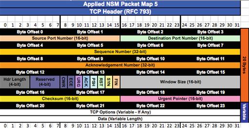
This is achieved by examining the TCP data offset field at the higher order nibble of 0×12. The value for this field is 5, but again, this is a computed field and must be multiplied by four to arrive at the real value. This means that the TCP header length is really 20 bytes.
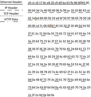
If you count off 20 bytes from the beginning of the TCP header, you will find that there is still data after the end of the header. This is application layer data. Unfortunately, TCP doesn’t have any sort of field that will tell us what application layer protocol to expect in the application, but something we can do is take a look at the destination port field (assuming that this is client to server traffic, otherwise we would look at the source port field) at 0×2:2 in the TCP header. This field has a value of 00 50, which converts to 80 in decimal. Since port 80 is typically used by the HTTP protocol, it might be the case that the data that follows is HTTP data. You could verify this by comparing the hex data with a protocol map of the HTTP protocol, or by just taking that data, from the end of the TCP header to the end of the packet, and converting it to ASCII text (Figure 13.17).
The protocol level break down of the packet we’ve just dissected is now shown in Figure 13.18.
Now, let’s talk about some tools that you can use to display and interact with packets.
Tcpdump for NSM Analysis
Tcpdump is a packet capture and analysis tool that is the de facto standard for command line packet analysis in Unix environments. It is incredibly useful as a packet analysis tool because it gets you straight to the data quickly, without a bunch of fuss. This makes it ideal for examining individual packets or communication sequences. It also provides consistent output, so packet data can be manipulated with scripts easily. Tcpdump is also included with a large number of Unix-based distributions, and can be installed easily via the operating systems packet manager software when it is not. Security Onion includes tcpdump out of the box.
The downside to tcpdump is that its simplicity means that it lacks some of the fancier analysis features that are included in a graphical tool like Wireshark. It has no concept of state, and it also doesn’t provide any ability to interpret application layer protocols.
In this section we won’t provide an extensive guide to every feature tcpdump has to offer, but we will provide the necessary jumpstart that a new NSM analyst needs to get moving in the right direction.
To start with, tcpdump has the ability to capture packets directly from the wire. This can be done by running tcpdump with no command line arguments, which will instruct tcpdump to capture packets from the lowest numbered network interface. In this case, tcpdump will output each packet it captures as a single summary line in the current terminal. To gain a bit more control over this process, we will use the –i argument so that we can specify the interface to capture packet on, and the –nn switch to turn off host and protocol name resolution.
If you’d like to save the packets you are capturing for analysis later, you can use the –w switch to specify the name of an output file where the data can be saved. Combining all of these arguments, we are left with the following command:
sudo tcpdump –nni eth1 –w packets.pcap
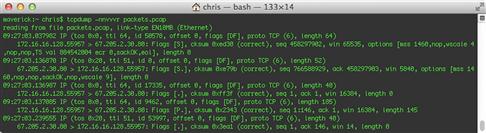
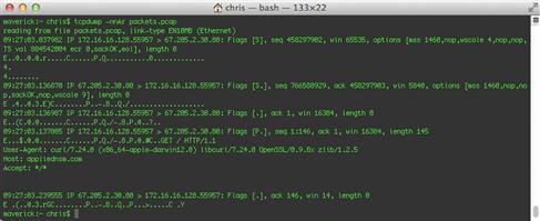
Now, if you want to read this file you can specify the –r command with the file name, shown in Figure 13.19.

The output tcpdump provides by default gives some basic information about each packet. The formatting of this output will vary based upon what protocols are in use, but the most common formats are:
TCP:
[Timestamp] [Layer 3 Protocol] [Source IP].[Source Port] > [Destination IP].[Destination Port]: [TCP Flags], [TCP Sequence Number], [TCP Acknowledgement Number], [TCP Windows Size], [Data Length]
UDP:
[Timestamp] [Layer 3 Protocol] [Source IP].[Source Port] > [Destination IP].[Destination Port]: [Layer 4 Protocol], [Data Length]
You can force tcpdump to provide more information in this summary line by adding the –v tag to increase its verbosity. You can further the verbosity by adding additional v’s, up to a total of three. Figure 13.20 shows the same packet from above, but with –vvv verbosity.
This is all very useful data, but it doesn’t give us the entire picture.
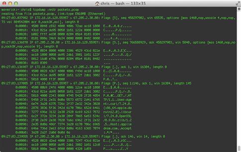
One way to display the entirety of each packet is to instruct tcpdump to output packets in hex format, with the –x switch, shown in Figure 13.21.
Another method is to display packets in ASCII, with the –A argument (Figure 13.22).
My personal favorite is the –X argument, which displays packets in both hex and ASCII, side by side (Figure 13.23).
In many cases, you will be dealing with larger PCAP files and it may become necessary to use filters to select only the data you wish to examine, or to purge data that isn’t valuable to the current investigation. Tcpdump utilizes the Berkeley Packet Filter (BPF) format. A filter can be invoked by tcpdump by adding it to the end of the tcpdump command. For easier readability, it is recommended that these filters be enclosed in single quotes. With this in mind, if we wanted to view only packets with the destination port TCP/8080, we could invoke this command:
tcpdump –nnr packets.pcap ‘tcp dst port 8080’
We could also take advantage of the –w argument to create a new file containing only the packets matching this filter:
tcpdump –nnr packets.pcap ‘tcp dst port 8080’ –w packets_tcp8080.pcap
In some cases, you might be using a large number of filtering options when parsing a packet capture. This commonly happens when an analyst is reviewing traffic and weeding out traffic from a large number of hosts and protocols that aren’t relevant to the current investigation. When this happens, it isn’t easy to edit these filters in the command line argument. Because of this, tcpdump allows for the use of the –F argument, which allows the user to specify a filter file that contains BPF arguments.
This command designates a filter file with the –F argument:
tcpdump –nnr packets.pcap –F known_good_hosts.bpf
We will talk about creating custom filters later in this chapter.
While this isn’t an exhaustive reference on tcpdump, it covers all of the primary uses that an analyst will usually encounter in the day-to-day parsing of packet data. If you want to learn more about tcpdump, you can visit http://www.tcpdump.org, or view the tcpdump manual pages by typing man tcpdump on a system with tcpdump installed.
TShark for Packet Analysis
The tshark utility is packaged with the Wireshark graphical packet analysis application as a command-line based alternative. It has a lot of the same abilities as tcpdump, but it has the added advantage of leveraging Wireshark’s protocol dissectors, which can be used to perform additional automated analysis of application layer protocols. This also allows for the use of Wireshark’s display filtering syntax, which adds some flexibility beyond that of Berkeley Packet Filters. This strength can also be a weakness in some cases, as the additional processing required to support these features means that tshark is generally slower than tcpdump when parsing data.
If you are using a system that has Wireshark installed, like Security Onion, then tshark is already installed and can be invoked by running the tshark command. The following command can be used to capture packets with tshark:
sudo tshark –i eth1
This command will display captured packets in the current terminal window, and will display a single one-line summary for each packet. If you’d like to save the packets you are capturing for analysis later, you can use the –w switch to specify an output file where the data can be saved. Combining all of these arguments, we are left with the following command:
sudo tshark –i eth1 –w packets.pcap
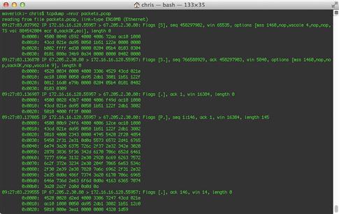
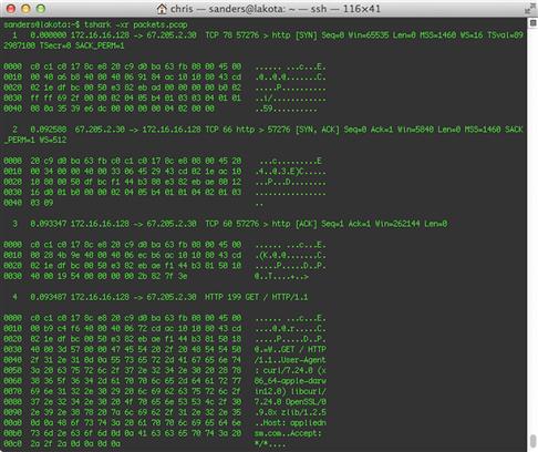
Now, if you want to read this file you can specify the –r command with the file name, shown in Figure 13.24.
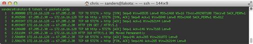
The formatting of this output will vary based upon what protocols are in use. In this case, notice that tshark is able to provide the additional functionality of showing application layer data in packets 4 and 6. This is possible because of its extensive collection of protocol dissectors. If you’d like a significantly more verbose output, including information obtained from tshark’s application layer protocol dissectors, you can add the –V argument. Figure 13.25 shows a portion of this output for a single packet.

Looking closely at the normal tshark output shown in Figure 13.20, you will notice that the timestamps look a little funny. Tshark’s default behavior is to display timestamps that are in relation to the beginning of the packet capture. To provide more flexibility, tshark provides the –t option so that you can specify alternate ways to display the timestamp. In order to print packets with timestamps that show the actual date and time the packet was captured, similar to tcpdump, use the –t ad option, as shown in Figure 13.26.
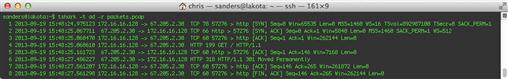
Using this feature, you can also choose to display packet timestamps as a delta, which is the time since the previous captured packet, using the –t d argument.
If you’d like to examine the raw packet data in a capture file, you can instruct tshark to output packets in hex and ASCII format using the –x argument, shown in Figure 13.27.
Tshark provides the ability to use both capture filters that use the same BPF syntax you are used to with tcpdump, and display filters that leverage tshark’s packet dissectors. The key distinction here is that capture filters can only be used while capturing packets, whereas display filters can also be used when reading packets from a file. To use capture filters, invoke the –f argument, followed by the filter you’d like to use. For example, the following command would limit a tshark capture to only UDP packets with the destination port 53, which would identify DNS traffic:
sudo tshark –I eth1 –f ‘udp && dst port 53’
If you’d like to use a display filter to perform the same filtering action on a capture file that’s being read, you can add this filter by specifying the –R argument, like this:
tshark –r packets.pcap –R ‘udp && dst.port == 53’
We will discuss tshark and Wireshark’s display filter syntax later in this chapter.
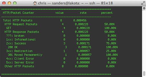
Another really useful feature provided by tshark is its ability to generate statistics based on the packet data that it sees. You can instruct tshark to generate statistics from a packet capture by invoking the –z option with the name of the statistic you wish to generate. A complete list of the statistical options is available by viewing the tshark manual page. This command uses the http,tree option, which displays a breakdown of HTTP status codes and request methods identified in the packet capture.
tshark –r packets.pcap –z http,tree
The output of this command is shown in Figure 13.28.
A few of my favorite statistical options available here are:
• io,phs: Displays a protocol hierarchy showing all protocols found within the capture file.
• http,tree: Displays statistics related to the types of HTTP Request and Response packets.
• http_req,tree: Displays statistics for every HTTP Request made.
• smb,srt: Displays statistics related to SMB commands. Useful for analyzing Windows SMB traffic.
Tshark is incredibly powerful, and is a useful tool for an NSM analyst in addition to tcpdump. In my analysis, I typically start with tcpdump so that I can filter through packets quickly based upon their layer three and four attributes. When I need to remain at the command line level and get more detail about a communication sequence in relation to application layer information, or to generate some basic statistics, I will usually call upon tshark. You can learn more about tshark by visiting http://www.wireshark.org or by viewing the tshark manual page by running man tshark on a system with tshark installed.
Wireshark for NSM Analysis
While command-line based packet analysis tools are ideal for interacting with packets at a fundamental level, some analysis tasks are best accomplished with a graphical packet analysis application like Wireshark. Wireshark was developed by Gerald Combs in 1998 under the project name Ethereal. The project was renamed Wireshark in 2006, and has grown tremendously thanks to the help of over 500 contributors since its inception. Wireshark is the gold standard for graphical packet analysis applications, and comes preinstalled on Security Onion.
If you aren’t using Security Onion, you can find instructions for installing Wireshark on to your platform at http://www.wireshark.org. Wireshark is a multi-platform tool, and works on Windows, Mac, and Linux systems. If you are using Security Onion, you can launch Wireshark from the command line by simply typing wireshark, or by clicking the Wireshark icon under the Security Onion heading in the desktop menu. If you need to be able to capture packets in addition to analyzing them, you will have to run Wireshark with elevated privileges using the command sudo wireshark. The Wireshark window is devoid of any useful information when it first opens, so we need to collect some packet data to look at.
Capturing Packets
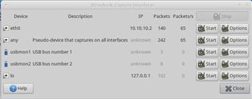
To capture packets from the wire, you can select Capture > Interfaces from the main drop-down menu. This will show all of the interfaces on the system (Figure 13.29). Here you can choose to capture packets from a sensor interface or another interface. To begin capturing packets from a particular interface, click Start next to that interface.
When you’ve finished collecting packets, click the Stop button under the Capture drop-down menu. At this point, you should be presented with data to be analyzed. In Figure 13.30, we’ve opened up one of the many packet capture files that come with Security Onion under the /opt/samples/ directory.
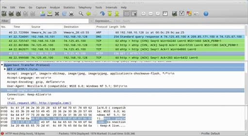
Looking at the image above, you will notice that Wireshark is divided into three panes. The uppermost is the packet list pane, which shows each packet summarized into a single line, with individual fields separated as columns. The default columns include a packet number, a timestamp (defaulting to the time since the beginning of the capture), source and destination address, protocol, packet length, and an info column that contains protocol-specific information.
The middle pane is the packet details pane, and shows detailed information about the data fields contained within the packet that is selected in the packet list pane. The bottom pane is the packet bytes pane, and details the individual bytes that comprise a packet, shown in hex and ASCII format, similar to tcpdump’s –X option.
The important thing to note when interacting with these three panes is that the data that each one displays is linked to actions taken in the other panes. When you click on a packet in the packet list pane, it shows data related to that packet in the packet details and packet bytes panes. Furthermore, when you click on a field in the packet details pane, it will highlight the bytes associated with that field in the packet bytes pane. This is ideal for visually bouncing around to different packets and determining their properties quickly.
Wireshark has a ton of features that are useful for analyzing packets. So many, as a matter of fact, that there is no way that we can cover them all in this chapter. If you want to read something that more exhaustively covers Wireshark and its features, I recommend my other book, “Practical Packet Analysis”, or Laura Chappell’s book, “Wireshark Network Analysis.” Both of these books cover packet analysis and TCP/IP protocols from a very broad perspective. With that said, there are a few nice features that are worth highlighting here. We will cover these briefly.
Changing Time Display Formats
Just like with Tshark, Wireshark will default to displaying packets with a timestamp that shows each packet relative to the number of seconds since the beginning of the packet capture. While this can be useful in certain situations, I typically prefer to see packets in relation to absolute time. You can change this setting from the main drop-down menu by selecting View > Time Display Format > Date and Time of Day. If the capture file you are working with contains packets from a single day, you can compact the size of your time column by selecting Time of Day instead.
Instead of having to change the time display format every time you open Wireshark, you can change the default setting by following these steps:
1. From the main drop-down menu, select Edit > Preferences.
Another time display format I find useful from time to time is the Seconds Since Previous Displayed Packet option. This can be useful when analyzing a solitary communication sequence and attempting to determine the time intervals between specific actions. This can be handy for determining if the actions of a process are being caused by human input or a script. Human actions are unpredictable, where as a script’s actions can be aligned with precise intervals.
Finally, in some cases it might be useful to know how long something has occurred after a previous event occurs. In these instances, Wireshark allows you to toggle an individual packet as time reference. This can be done by right clicking on a packet and selecting Set Time Reference (toggle). With this set, change your time display format back to Seconds Since Beginning of Capture, and packets following the packet you’ve toggled will reference the number of seconds since that packet has occurred. Multiple packets can be selected as time reference packets.
Capture Summary
The first thing I typically do when I open any packet capture in Wireshark is to open the Summary window by selecting Statistics > Summary from the main drop-down menu. This screen, shown in Figure 13.31, provides a wealth of information and statistics about the packet capture and the data contained within it.
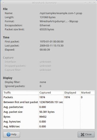
The important items on this screen for the analyst include:
• Format: The format of the file. If you are dealing with a PCAP-NG file, you know that you can add comments to packets.
• Time: This section includes the time the first packet was captured, the time the last packet was captured, and the duration between those times. This is critical in confirming that the capture contains the time frame associated with the current investigation.
• Bytes: The size of the data in the capture file. This gives you an idea of how much data you are looking at.
• Avg. Packet Size: The average size of the packets in the capture file. In some cases, this number can be used to ascertain the makeup of the traffic in the capture file. For instance, a larger average would indicate more packets containing data, and a smaller average would indicate more control/command packets generated at the protocol level. Keep in mind that this isn’t always the most reliable indicator, and is something that can vary wildly depending on a variety of factors.
• Avg. Bytes/sec and Avg. Mbit/sec: The average number of bytes/megabits per second occurring in the capture. This is useful for determining the rate at which communication is occurring.
Protocol Hierarchy
The protocol hierarchy screen is accessible by selecting Statistics > Protocol Hierarchy from the main drop-down menu. It will provide a snapshot of every protocol found within the capture file, along with a statistical breakdown that will help you to determine the percentage of traffic associated with each protocol in the capture file.
This statistical feature is often another first stop when performing analysis of a packet capture. Because of its concise view of the data, you can quickly identify abnormal or unexpected protocols that warrant further analysis, such as an instance where you see SMB traffic, but you have no Windows or Samba hosts on a network segment. You can also use this feature to find odd ratios of expected protocols. For instance, seeing that the packet capture contains an unusually high percentage of DNS or ICMP traffic might mean those packets warrant further investigation.
You can create display filters directly from this window by right clicking on a protocol, selecting Apply As Filter, and then selecting a filter option. The Selected option will only show packets utilizing that protocol, where as the Not Selected option will show packets not utilizing that protocol. Several other options are available that can be used to build compound display filters.
Endpoints and Conversations
In Wireshark terms, a device that communicates on the network is considered to be an endpoint, and when two endpoints communicate they are said to be having a conversation. Wireshark provides the ability to view communication statistics for individual endpoints and for communication between endpoints.
You can view endpoint statistics by selecting Statistics > Endpoints from the main drop-down menu. This screen is shown in Figure 13.33.


Conversations can be accessed in a similar manner by selecting Statistics > Conversations from the main drop-down menu. This screen is shown in Figure 13.34.

Both of these windows have a similar layout, and list each endpoint or conversation on a new line, complete with statistics regarding the number of packets and bytes transmitted in each direction. You should also notice that each window has a number of tabs across the top that represent different protocols operating on multiple layers. Wireshark breaks down endpoints and conversations by these protocols and the addresses used on these layers. Because of this, a single Ethernet endpoint could actually be tied to multiple IPv4 endpoints. Likewise, a conversation between several IP addresses could actually be limited to only two physical devices, each having a single Ethernet MAC address.
The endpoints and conversations windows are useful for determining who the key role players are in a capture file. Here you can see which hosts transmit and receive the most or least amount of traffic, which can help you narrow down the scope of your investigation. Just like with the protocol hierarchy window, you can create filters directly from these screens by right clicking on an endpoint or conversation.
Following Streams
We’ve already seen how Wireshark can delineate traffic that occurs as a part of a conversation between two endpoints, but often we are more concerned about the content of the data being exchanged between these devices rather than merely the list of packets associated with the communication sequence. Once you’ve created a filter that only shows the traffic in a conversation, you can use Wireshark’s stream following options to get a different viewpoint on the application layer data contained in those packets. In this case, this can be done by right clicking on a TCP packet, and selecting Follow TCP Stream.
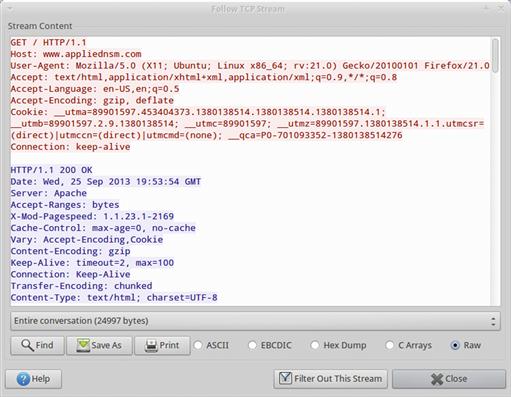
The figure above shows the TCP Stream output of an HTTP connection. As you can see, Wireshark has taken the application layer data contained in this conversation’s packets and has reassembled them in a manner that excludes all of the lower layer information. This allows us to quickly see what is going on in this HTTP transaction. You can choose to output this information in a variety of formats, and you can also only show communication from a single direction if you choose.
Wireshark also provides the functionality to perform this same action with UDP and SSL streams. The amount of value you will obtain from following streams varies depending upon the application layer protocol in use, and of course, following encrypted streams like HTTPS or SSH connection often won’t yield a ton of value.
IO Graph
You are able to see the average throughput of the data contained in a packet capture by using the Wireshark Summary dialog that we looked at earlier. This is great for an overall average throughput measurement, but if you want to ascertain the throughput of packets in a capture at any given point in time, you will need to use Wireshark to generate an IO graph. These graphs allow you to display the throughput of data in a capture file over time (Figure 13.36).

The figure above shows a basic throughput graph for a single packet capture. In this case, there is a line showing throughput for all of the packets contained in the capture file (Graph 1), and two more lines showing throughput for packets that match display filters. One of these display filters shows all HTTP traffic contained in the capture (Graph 3), and the other shows traffic generated from a specific host with the IP address 74.125.103.164 (Graph 4).
The IO graph provides the ability to change the units and intervals used by the graph. I tend to use Bytes/tick as my unit, and will scale the unit intervals with the size of the data I’m looking at.
IO Graphs are useful for examining the amount of traffic generated by certain devices or protocols, or for quickly identifying spikes in the amount of traffic associated with a particular type of communication.
Exporting Objects
Wireshark has the ability to detect the transfer of individual files inside of certain protocols. Because of this, it also has the ability to export these files from the packet capture, assuming the capture includes the entire data stream that contains the file. As of the writing of this book, Wireshark supports exporting objects from HTTP, SMB, and DICOM streams.
If you’d like to experiment with this functionality, you can try the following steps:
1. Start a new packet capture in Wireshark. Choose the network interface associated with the device you running Wireshark on.
2. Open a browser and visit a few different websites.
4. From Wireshark’s main drop-down menu, select File > Export > Objects > HTTP
5. A list will be displayed that shows the files Wireshark has detected in the communication stream (Figure 13.37). Click on the object you would like to export, and select Save As. You can then select the location where the file should be stored and provide the name of the file to save it.
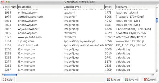
Figure 13.37 Selecting an HTTP Object to Export
Remember that to be able to extract a file properly from a packet capture, you must have every packet associated with that file’s transfer across the network.
This feature of Wireshark is incredibly valuable. While there are other options for exporting files from packet data streams, such as Bro’s File Analysis Framework, being able to do this directly from Wireshark is very convenient. I use this feature often when I see a suspicious file going across the wire. Just be careful with any file you export, as it could be malicious and you might end up infecting yourself with some type of malware or something else that might cause other harm to your system.
Adding Custom Columns
In a default installation, Wireshark provides 7 columns in the packet list pane. These are the packet number, time stamp, source address, destination address, protocol, length, and info fields. These are certainly essentials, but it is often the case that adding additional columns to this pane can enhance analysis. There are a couple of ways to do this, and to demonstrate both methods we will add three new columns to the packet list pane: source and destination port number and HTTP method.
We will begin by adding the source and destination port number. While the source and destination port number values are generally shown in the Info field, having them as their own column so that you can identify and sort by them easily is convenient. This is also useful for identifying different streams.
We will add these columns using the Wireshark Preferences dialog, which involves these steps:
1. From Wireshark’s main drop-down menu, select Edit > Preferences.
2. Select the Columns option on the left side of the screen.
3. Click the Add button, and select the Source Port (unresolved) option in the Field Type dialog.
4. Double click “New Column” on the newly added field, and replace that title with “SPort.”
5. Click the Add button, and select the Dest Port (unresolved) option.
6. Double click “New Column” on the newly added field, and replace that title with “DPort”.
7. Drag the SPort field so that it is placed after the Source field.
8. Drag the DPort field so that it is placed after the Destination field
10. When you are finished, the Columns screen should look similar to Figure 13.38.

Figure 13.38 The Columns Screen with Newly Added Fields
Next, we will add the HTTP Method column. This field isn’t something that you will want taking up screen real estate all the time, but it is useful when analyzing HTTP traffic so that you can quickly identify packets representing HTTP GET or POST commands. Instead of adding this field using the same method as before, we will add it from the main Wireshark window using the following steps:
1. Start a new packet capture in Wireshark. Choose the network interface associated with the device you running Wireshark on.
2. Open a browser and visit a few different websites.
4. Find an HTTP packet that contains an HTTP Request Method, such as a GET or POST packet. This can be done manually, or with the help of the display filter http.request.
5. Select the packet in the packet list pane, and then expand the HTTP protocol header information portion of the packet in the packet details pane. Drill down until you find the Request Method field.
6. Right click the Request Method field and select “Apply as Column”.
The Request Method column should now be inserted right before the Info column. If you’d like to change the position of the column, you can click and drag it to the left or right of the other columns. You can edit the name and other attributes of the column by right clicking it and selecting Edit Column Details. If you decide that you want to get rid of a column you can remove it by right clicking the column header and choosing Remove Column.
Columns added using either of these methods will be added to the profile currently in use, so when you close Wireshark and relaunch it, the columns you have added will remain. Some columns, such as source and destination port, are something I use in most every scenario. Other columns like the HTTP Request Method are situational, and I will usually add and remove those at will depending on the type of traffic I am examining. You can turn virtually any field from a dissected packet into a column in Wireshark by right-clicking that field and choosing Apply as Column. This is a feature you shouldn’t be afraid to use liberally!
Configuring Protocol Dissector Options
Perhaps the most exciting feature offered by Wireshark is the vast number of protocol dissectors. Protocol dissectors are modules that Wireshark uses to parse individual protocols so that they can be interpreted on a field-by-field basis. This allows the user to create filters based upon specific protocol criteria. Some of these protocol dissectors have options that can be useful in changing the way that analysis is performed.
You can access the protocol dissector options from the main drop-down menu by selecting Edit > Preferences, and then expanding the Protocols header. The list that is provided shows every protocol dissector loaded into Wireshark. If you click on one of these protocols, you will be presented with its options on the right hand side of this window. Figure 13.39 shows the protocol dissector options for the TCP protocol.
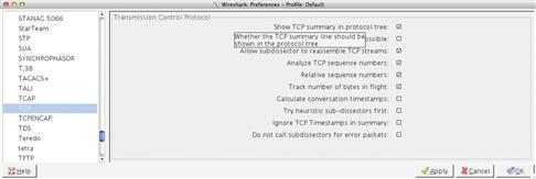
Examining the protocol dissector options for common protocols is a useful way to gain insight into how Wireshark obtains some of the information it presents. For instance, in the figure above you will notice that, by default, Wireshark will display relative sequence numbers for TCP connections rather than absolute sequence numbers. If you didn’t know this and were to look at the same set of packets in another application expecting to locate a particular sequence number, you might be alarmed to find that the number you were expecting doesn’t exist. In that case, you could disable relative sequence numbers here to get the real TCP sequence numbers. If you spend a lot of time at the packet level, then you will probably want to take some time to examine the protocol dissector options for the major TCP/IP protocols and other protocols you work with on a regular basis.
Capture and Display Filters
Wireshark allows for the use of BPF formatted capture filters, as well as display filters that use its own custom syntax designed to interact with fields generated by protocol dissectors.
Capture filters in BPF format can be applied to Wireshark only while capturing data. To use a capture filter, select Capture > Options from the main drop-down menu. Then, double-click the interface you plan to perform the capture on. Finally, place your capture filter into the Capture Filter dialog area (Figure 13.40) and click OK. Now, when you click Start on the previous screen, the capture filter will be applied and the packets not matching the filter will be discarded. In this example, we’ve applied a filter that matches any packets from the source network 192.168.0.0/24 that are not using port 80. Make sure to remember to clear out capture filters when you are done with them, otherwise you might not be collecting all of the packets you expect.

Display filters can be applied by typing them directly into the filter dialog above the packet list pane in the main Wireshark window. Once you’ve typed a filter into this area, click Apply to show only the packets matching that filter. When you’d like to remove the filter, you can click the Clear options. You can locate advanced filtering options by using Wireshark’s expression filter. This is done by clicking the Expression button next to the display filter dialog box (Figure 13.41).
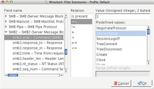
In the figure above, we’ve selected a filter expression option that will match SMB2 SessionSetup requests.
This section demonstrated how to apply capture and display filters in Wireshark. In the next section we will discuss the process of creating these filters for use during collection, detection, and analysis.
Packet Filtering
Capture and display filters allow you to specify which packets you want to see, or the ones you don’t want to see, when interacting with a capture file. When analyzing packets, the majority of your time will be spent taking larger data sets and filtering them down into manageable chunks that are valuable in the context of an investigation. Because of this, it is critical that you understand packet filtering and how it can be applied to a variety of situations. In this section we will look at two types of packet filtering syntaxes: Berkeley Packet Filters (Capture Filters) and Wireshark/tshark Display Filters.
Berkeley Packet Filters (BPFs)
The BPF syntax is the most commonly used packet filtering syntax, and is used by a number of packet processing applications. Tcpdump uses BPF syntax exclusively, and Wireshark and tshark can use BPF syntax while capturing packets from the network. BPFs can be used during collection in order to eliminate unwanted traffic, or traffic that isn’t useful for detection and analysis (as discussed in Chapter 4), or they can be used while analyzing traffic that has already been collected by a sensor.
BPF Anatomy
A filter created using the BPF syntax is called an expression. These expressions have a particular anatomy and structure, consisting of one or more primitives that can be combined with operators. A primitive can be thought of as a single filtering statement, and they consist of one or more qualifiers, followed by a value in the form of an ID name or number. An example of this expression format is shown in Figure 13.42, with each component labeled accordingly.
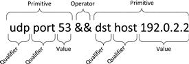
In the example shown above, we have an expression that consists of two primitives, udp port 53 and dst host 192.0.2.2. The first primitive uses the qualifiers udp and port, and the value 53. This primitive will match any traffic to or from port 53 using the UDP transport layer protocol. The second primitive uses the qualifiers dst and host, and the value 192.0.2.2. This primitive will match any traffic destined to the host with the IP address 192.0.2.2. Both primitives are combined with the concatenation operator (&&) to form a single expression that evaluates to true when a packet matches both primitives.
BPF qualifiers come in three different types. These types, along with an example of qualifiers for each type are shown in Table 13.1.
Table 13.1
| Qualifier Type | Qualifier | Description |
| Type | Identifies what the value refers to. “What are you looking for?” | |
| host | Specify a host by IP address | |
| net | Specify a network in CIDR notation | |
| port | Specify a port | |
| Dir | Identifies the transfer direction to or from the value. “What direction is it going?” | |
| src | Identify a value as the communication source | |
| dst | Identify a value as the communication destination | |
| Proto | Identifies the protocol in use. “What protocol is it using?” | |
| ip | Specify the IP protocol | |
| tcp | Specify the TCP protocol | |
| udp | Specify the UDP protocol |
As you can see in the example shown in Figure 13.1, qualifiers can be combined in relation to a specific value. For example, you can specify a primitive with a single qualifier like host 192.0.2.2, which will match any traffic to or from that IP address. Alternatively, you can use multiple qualifiers like src host 192.0.2.2, which will match only traffic sourced from that IP address.
When combining primitives, there are three logical operators that can be used, shown here (Table 13.2):
Table 13.2
| Operator | Symbol | Description |
| Concatenation (AND) | && | Evaluates to true when both conditions are true |
| Alternation Operator (OR) | || | Evaluates to true when either condition is true |
| Negation Operator (NOT) | ! | Evaluates to true when a condition is NOT met |
Now that we understand how to create basic BPF expressions, I’ve created a few basic examples in Table 13.3.
Table 13.3
| Expression | Description |
| host 192.0.2.100 | Matches traffic to or from the IPv4 address specified |
| dst host 2001:db8:85a3::8a2e:370:7334 | Matches traffic to the IPv6 address specified |
| ether host 00:1a:a0:52:e2:a0 | Matches traffic to the MAC address specified |
| port 53 | Matches traffic to or from port 53 (DNS) |
| tcp port 53 | Matches traffic to or from TCP port 53 (Large DNS responses and zone transfers) |
| !port 22 | Matches any traffic not to or from port 22 (SSH) |
| icmp | Matches all ICMP traffic |
| !ip6 | Matches everything that is not IPv6 |
Filtering Individual Protocol Fields
You can do some pretty useful filtering using the syntax we’ve learned up until this point, but using this syntax alone limits you to only examining a few specific protocol fields. One of the real benefits of the BPF syntax is that it can be used to look at ANY field within the headers of the TCP/IP protocols.
As an example, let’s say that you would like to examine the Time to Live (TTL) value in the IPv4 header to attempt to filter based upon the operating system architecture of a device that is generating packets. While it isn’t always an exact science and it can certainly be fooled, Windows devices will generally use a default initial TTL of 128, and Linux devices will generally use a TTL of 64. This means that we can do some rudimentary passive operating system detection with packets. To do this, we will create a BPF expression that looks for values in the TTL field that are greater than 64.
To create this filter, we have to identify the offset where the TTL field begins in the IP header. Using a packet map, we can determine that this field begins at 0x8 (remember to start counting from 0). With this information, we can create a filter expression by telling tcpdump which protocol header to look in, and then specifying the byte offset where the value exists inside of square brackets. This can be combined with the greater than (>) logical operator and the value we’ve selected. The end result is this BPF expression:
ip[8] > 64
The expression above will instruct tcpdump (or whatever BPF-aware application you are using) to read the value of the eighth byte offset from 0 in the TCP header. If the value of this field is greater than 64, it will match. Now, let’s look at a similar example where we want to examine a field that spans multiple bytes.
The Window Size field in the TCP header is used to control the flow of data between two communicating hosts. If one host becomes too overloaded with data and its buffer space fills up, it will send a packet to the other host with a window size value of 0 to instruct that host to stop sending data so that it can catch up. This process helps ensure reliable delivery of data. We can detect the TCP zero window packets by creating a filter to examine this field.
Using the same strategy as before, we have to look at a packet map to determine where this field is located in the TCP header. In this case, the field occurs at byte 0x14. In this case, note that this field is actually two bytes in length. We can tell tcpdump that this is a two byte field by specifying the offset number and byte length inside of the square brackets, separated by a colon. Doing this, we are left with this expression:
tcp[14:2] = 0
This expression tells tcpdump to look at the TCP header and to examine the 2 bytes occurring starting at the fourteenth byte offset from 0. If the value of this field is 0, the filter expression will match. Now that we know how to examine a field longer than a byte, let’s look at examining fields shorter than a byte.
The TCP protocol uses various flags to indicate the purpose of each packet. For instance, the SYN flag is used by packets that initialize a connection, while the RST and FIN packets are used for terminating a connection in an abrupt or graceful manner, respectively. These flags are individual 1-bit fields contained within byte 0x13 in the TCP header.
To demonstrate how to create filters matching fields smaller than a byte, let’s create an expression that matches any TCP packet that has only the RST flag enabled. This will require a few steps toward the creation of a bit masked expression.
First, we should identify the value we want to examine within the packet header. In this case, the RST flag is in byte 0x13 in the TCP header, in the third position in this byte (counting from right to left). With that knowledge in mind, it becomes necessary to create a binary mask that tells tcpdump which bits in this field we actually care about.
The field we want to examine in this byte is in the third position, so we place a 1 in the third position of our bit mask and place 0’s in the remaining fields. The result is the binary value 00000100.
Next, we have to translate this value into its hexadecimal representation. In this case, 00000100 breaks down as 0x04 in hex.
Now we can build our expression by specifying the protocol and byte offset value for 0x13, followed by an ampersand (&) and the byte mask value we just created.
tcp[13] & 0x04
Finally, we can provide the value we want to match in this field. In this case, we want any packet that has a 1 set in this field. Since a 1 in the third position of a byte equals 4, we can simply use 4 as the value to match.
tcp[13] & 0x04 = 4
This expression will match any packet with only the TCP RST bit set.
There are a number of different applications for BPF expressions that examine individual protocol fields. For example, the expression icmp[0] == 8 || icmp[0] == 0 can be used to match ICMP echo requests or replies. Given the examples in this section, you should be able to create filter expressions for virtually any protocol field that is of interest to you. Next, we will look at display filters.
Wireshark Display Filters
Wireshark and tshark both provide the ability to use display filters. These are different than capture filters, because they leverage the protocol dissectors these tools use to capture information about individual protocol fields. Because of this, they are a lot more powerful. As of version 1.10, Wireshark supports around 1000 protocols and nearly 141000 protocol fields, and you can create filter expressions using any of them. Unlike capture filters, display filters are applied to a packet capture after data has been collected.
Earlier we discussed how to use display filters in Wireshark and tshark, but let’s take a closer look at how these expressions are built, along with some examples.
A typical display filter expression consists of a field name, a comparison operator, and a value.
A field name can be a protocol, a field within a protocol, or a field that a protocol dissector provides in relation to a protocol. Some example field names might include the protocol icmp, or the protocol fields icmp.type and icmp.code. A complete list of field names can be found by accessing the display filter expression builder (described in the Wireshark section of this chapter) or by accessing the Wireshark help file. Simply put, any field that you see in Wireshark’s packet details pane can be used in a filter expression.
Next is the comparison operator (sometimes called a relational operator), which determines how Wireshark compares the specified value in relation to the data it interprets in the field. The comparison operators Wireshark supports are shown in Table 13.4. You can alternate use of the English and C-like operators based upon what you are comfortable with.
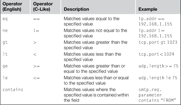
The last element in the expression is the value, which is what you want to match in relation to the comparison operator. Values also come in different types as well, which are shown in Table 13.5.
Table 13.5
| Value Type | Description | Example |
| Integer (Signed or Unsigned) | Expressed in decimal, octal, or hexadecimal | tcp.port == 443 ip.proto == 0x06 |
| Boolean | Expressed as true (1) or False (0) | tcp.flags.syn == 1 ip.frags.mf == 0 |
| String | Expressed as ASCII text | http.request.uri == “http://www.appliednsm.com” smtp.req.parameter contains “FROM” |
| Address | Expressed as any number of addresses: IPv4, IPv6, MAC, etc. | ip.src == 192.168.1.155 ip.dst == 192.168.1.0/24 ether.dst == ff:ff:ff:ff:ff:ff |
Now that we understand how filters are constructed, let’s build a few of our own. Starting simple, we can create a filter expression that only shows packets using the IP protocol by simply stating the protocol name:
ip
Now, we can match based upon a specific source IP address by adding the src keyword to the expression:
ip.src == 192.168.1.155
Alternatively, we could match based upon packets with the destination IP address instead:
ip.dst == 192.168.1.155
Wireshark also includes custom fields that will incorporate values from multiple other fields. For instance, if we want to match packets with a specific IP address in either the source or destination fields, we could use this filter, which will examine both the ip.src and ip.dst fields:
ip.addr == 192.168.1.155
Multiple expressions can be combined using logical operators. These are shown in Table 13.6.
Table 13.6
Display Filter Logical Operators
| Operator (English) | Operator (C-Like) | Description |
| and | && | Evaluates to true when both conditions are true |
| or | || | Evaluates to true when either condition is true |
| xor | ^^ | Evaluates to true when one and only one condition is true |
| not | ! | Evaluates to true when a condition is NOT met |
We can combine a previous expression with another expression to make a compound expression. This will match any packets sourced from 192.168.1.155 that are not destined for port 80:
ip.src == 192.168.1.155 && !tcp.dstport == 80
Once again, the key thing to keep in mind when creating display filters is that anything you see in the packet details pane in Wireshark can be used in a filter expression. Table 13.7 contains a few more example display filter expressions.
Table 13.7
Example Display Filter Expressions
| Filter Expression | Description |
| eth.addr ! = < MAC address > | Match packets not to or from the specified MAC address. Useful for excluding traffic from the host you are using. |
| ipv6 | Match IPv6 packets |
| ip.geoip.country == < country > | Match packets to or from a specified country |
| ip.ttl < = < value > | Match packets with a TTL less than or equal to the specified value. This can be useful for some loose OS fingerprinting. |
| ip.checksum_bad == 1 | Match packets with an invalid IP checksum. Can be used for TCP and UDP checksums as well by replacing ip in the expression with udp or tcp. Useful for finding poorly forged packets. |
| tcp.stream == < value > | Match packets associated with a specific TCP stream. Useful for narrowing down specific communication transactions. |
| tcp.flags.syn == 1 | Match packets with the SYN flag set. This filter can be used with any TCP flag by replacing the “syn” portion of the expression with the appropriate flag abbreviation. |
| tcp.analysis.zero_window | Match packets that indicate a TCP window size of 0. Useful for finding hosts whose resources have become exhausted. |
| http.request == 1 | Match packets that are HTTP requests. |
| http.request.uri == “<value>” | Match HTTP request packets with a specified URI in the request. |
| http.response.code == < value > | Match HTTP response packets with the specified code. |
| http.user_agent == “value” | Match HTTP packets with a specified user agent string. |
| http.host == “value” | Match HTTP packets with a specified host value. |
| smtp.req.command == “<value > “ | Match SMTP request packets with a specified command |
| smtp.rsp.code == < value > | Match SMTP response packets with a specified code |
| smtp.message == “value” | Match packets with a specified SMTP message. |
| bootp.dchp | Match DHCP packets. |
| !arp | Match any packets that are not ARP. |
| ssh.encrypted_packet | Match encrypted SSH packets. |
| ssh.protocol == “<value>” | Match SSH packets of a specified protocol value. |
| dns.qry.type == < value > | Match DNS query packets of a specified type (A, MX, NS, SOA, etc). |
| dns.resp.type == < value > | Match DNS response packets of a specified type (A, MX, NS, SOA, etc). |
| dns.qry.name == “<value>” | Match DNS query packets containing the specified name. |
| dns.resp.name == “<value>” | Match DNS response packets containing the specified name. |
You should spend some time experimenting with display filter expressions and attempting to create useful ones. A quick perusal of the expression builder in Wireshark can point you in the right direction.
Conclusion
In this chapter we discussed the basics of packet analysis from a fundamental level. This journey began with an introduction to reading packets in hex with a primer in packet math. This led into an overview of tcpdump and tshark for packet analysis from the command line, and Wireshark as a graphical packet analysis platform. Finally, we discussed the anatomy and syntax of capture and display filters. Packet analysis is one of the most important skills an NSM analyst can have, so the knowledge in this chapter is incredibly important. Once you’ve mastered these concepts, you can look into some of the additional packet analysis resources mentioned at the start of the chapter to gain a deeper understanding of how packets work and the TCP/IP protocols.