Chapter 13. Growth Structures*
* For all figures in this chapter (in the printed book only), see the preface for information about registering your copy on the InformIT site for access to the electronic versions in color.
Introduction
Tectonic and sedimentary growth is important to petroleum exploration. For example, growth along faults creates both structural traps and seals (Brenneke 1995), and this growth can be coincident with the deposition of reservoir units. Growth faults may trap hydrocarbons during the early stages of a hydrocarbon cycle. The expanded sections that typically form downthrown to down-to-the-basin normal faults are the highest growth sections found in the petroleum regime (Thorsen 1963). These expanded downthrown sections often contain large accumulations of hydrocarbons (Tearpock et al. 1994). Hydrocarbon accumulations correlate not only to high growth intervals but often to the highest growth intervals within the petroleum system (Fisher and McGowen 1967; Woodbury et al. 1973; Branson 1991; Pacht et al. 1992). Therefore, in order to find large accumulations of hydrocarbons, we must understand and analyze growth. Also, growth defines the history of prospect formation.
We emphasized the importance of constructing a 3D structural framework in Chapters 7, 8, and 9. In this chapter we address the 4D time factor, which is important when exploring for and developing hydrocarbons. We consider the time variable through the superposition, or relative age, principle. In other words, the oldest rocks are the deepest rocks, except for the inverted sequences discussed in Chapter 10. Rocks record cycles of changing sedimentary influx that relate to systems tract and sequence boundaries. For example, if we define the thickness of an interval of sediments as d, and time as t, then the sedimentation rate is d/t. The sedimentation rate for that interval may change between two locations, and the change in rate is ∆d/t. We can take the ratio of the change in sedimentation rate to the sedimentation rate, or (Δd/t)/(d/t). In this ratio, time cancels out. This dimensionless growth (Suppe et al. 1992), or relative age, ratio Δd/d is a measure of growth (Bischke 1994b). When using subsurface data, information on growth and relative age is always available to evaluate growth and its impact on exploration.
We demonstrate from correlation data that each sedimentary sequence, being a genetically related unit, experiences different patterns of growth. Furthermore, sedimentary sequences in all tectonically active regimes exhibit growth, not just in the extensional growth fault regime. Typically, linear or monotonic patterns of growth characterize sedimentary sequences. The linear growth recorded in a sequence is typically punctuated by abrupt changes in growth rate. These punctuated growth patterns may aid in defining systems tract and sequence boundaries, and they can contribute to the resolution of a variety of practical problems involving changes in growth.
When geoscientists think of growth faulting, they are often referring to the large listric, growth normal faults. However, growth faults can be small, with only tens of feet of vertical displacements. Any normal fault is a growth fault if the stratigraphic section expands across the fault (Thorsen 1963; Dawers and Underhill 2000). Furthermore, all structural styles can exhibit growth, including growth reverse and growth thrust faults (Suppe et al. 1992) as well as growth strike-slip faults (Shaw et al. 1994; see Chapter 12) and growth inversion structures (Mitra 1993; Link et al. 1996). In this chapter, we discuss these and other complex structural styles that are sometimes misidentified with well log and seismic data. Structural styles are important because the recognition of the correct style for a region affects our interpretations and our understanding of the petroleum system. We discuss techniques for recognizing structural styles using growth analysis, with examples of growth structures from the four major tectonic regimes: extensional, compressional, strike-slip, and salt. Large accumulations of hydrocarbons correlate to timing of migration and fault movement, so it is important to understand the timing related to fault growth and deposition.
The methods presented in this chapter, the expansion index method (Thorsen 1963) and the high-resolution Δd/d technique and its related methods (Bischke 1994b; Sanchez et al. 1997), can have a high resolution, about one part in a thousand, and are robust (Chatellier and Porras 2001, 2004) when integrated with other geological and geophysical data, thus providing a check on existing interpretations. Growth analysis has helped resolve a number of existing or potential problems that include (1) rapidly distinguishing faults from unconformities on the flanks of salt bodies (Bischke et al. 1999) and confirming small faults or uncertain fault interpretations; (2) locating sequence boundaries (Bischke 1994b; Sanchez et al. 1997) and subtle stratigraphic traps and predicting erosional surfaces and potential bald structures on the crests of anticlines; (3) solving general correlation problems (discussed in this chapter); (4) calculating sand/shale ratios from seismic sections downthrown to normal faults (Pochat et al. 2004) and predicting major lithology from growth sections (Castelltort et al. 2004); (5) locating the highest growth or highest petroleum potential intervals (i.e., the thickest sands) (Fisher and McGowen 1967; Woodbury et al. 1973; Branson 1991; Pacht et al. 1992); (6) determining the time of structural growth and timing of faults (Cartwright et al. 1998, Echavarria and Allmendinger 2003); (7) checking interpretations for consistency with the existing growth history; (8) recognizing unidentified problems; and (9) quality-controlling the input values in a well log data base. The method has also been applied to determine timing on strike-slip faults (Shaw et al. 1994) and reverse and thrust faults (Echavarria et al. 2003). More recently, Chatellier and Rueda (2010) used these techniques to recognize missing section resulting from miscorrelations and for locating missing section on about the same structural level on a contractional folded structure. The missing section data contour into a shallow-dipping fault surface. This is consistent with a folded anticline subsequently faulted by another period of thrusting.
In this chapter, we describe practical examples pertaining to sequence stratigraphic interpretations, to strike-slip and compressional deformation, to unconformities and correlation problems related to salt, and to the extensional regime that typically contains growth sediments.
Expansion Index for Growth Faults
Thorsen (1963) proposed the expansion index method to categorize growth along normal faults. Indeed, the term expansion fault comes from Thorsen’s classic work on growth faulting. The expansion index is a ratio calculated by comparing a downthrown stratigraphic thickness to its correlative upthrown thickness. Evaluation of the indices for a sequence of stratigraphic units determines the timing and activity on growth faults, and a plot of the indices provides a record of the movement of a fault throughout its history. Although Thorsen (1963) developed the technique by studying growth faults in southeast Louisiana, USA, his method for analyzing growth faults applies to any region of the world that contains syntectonic faults.
For normal faults, the procedure starts by determining the correlative upthrown and downthrown stratigraphic units, and then comparing the thickness of each unit in the upthrown (footwall) and downthrown (hanging wall) blocks. By definition,
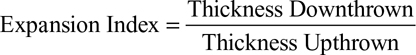
Where growth is recognized, an expansion index greater than 1.0 typifies growth. If the expansion index ratio is less than 1.0, then a correlation error has been made or an unconformity is present in the hanging wall fault block.
Figure 13-1 is a simple example to illustrate the determination and application of the expansion index for a generic growth fault. The left side of the figure contains a cross section of a growth fault with one well in the upthrown block and one in the expanded, downthrown block. For simplicity, the correlative horizons, a through k, in the upthrown fault block bound units that are all of equal thickness (t = 1.0). The thickness of each unit in the downthrown block is used to calculate the expansion index for each.
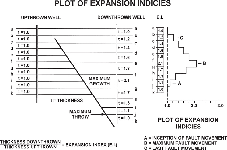
Figure 13-1 Expansion index can be used to measure the timing and rate of movement along a growth fault. Expansion indices are commonly illustrated in bar graph form (right side of figure). (From Thorsen 1963. Published by permission of the Gulf Coast Association of Geological Societies.))
Thorsen presents the results in the form of a bar graph on the right side of Figure 13-1, and the fault movement with time is readily apparent. By analyzing the graph of the expansion indices, we conclude that movement on the fault began at time j and reached a maximum period of growth activity between times f and g. Fault movement ceased at time b. The maximum period of fault growth between times f and g involved a 2.1 to 1 expansion of the downthrown stratigraphic section. If the interval f to g contains thick sands, then this thick interval has the highest potential for hydrocarbon accumulation.
Each growth fault appears to have its own unique fingerprint in reference to its expansion indices. The rate of movement on a growth fault increases from the initial movement to some maximum rate, and then decreases again until fault movement ceases. During its life, a growth fault may move sporadically, resulting in an irregular growth history. Each growth fault has its own unique growth history as a result of fault movement, the rate of subsidence, and the rate of sediment supply across the fault. Even over long horizontal distances, the fingerprint for a particular fault can usually be recognized along strike, as shown in Figure 13-2, even though the values of the expansion indices may not be constant along strike. The plots of the expansion indices for this fault, calculated at separate locations two miles apart, are similar. A review of the individual expansion indices and the overall pattern at each location shows that they are similar enough to be identified as representing the same fault.

Figure 13-2 Comparison of expansion indices, taken over 2 mi apart, indicates that a growth fault’s fingerprint can be recognized over long distances. (From Thorsen 1963. Published by permission of the Gulf Coast Association of Geological Societies.)
Because of the unique characteristics of the plot of the expansion indices for each growth fault, the technique can be used in complexly faulted areas as a lateral correlation tool for the identification of individual growth faults over long distances. The expansion index technique is applicable for use with either electric well logs or seismic sections. Because of the greater stratigraphic detail that is found in well logs versus seismic sections, expansion indices calculated using well logs are more accurate. One important note needs to be made with regard to this technique and seismic sections. As time distorts vertical distance on seismic sections, always depth-convert the seismic sections before calculating the expansion index.
The expansion index also serves as a vertical correlation aid for well log and seismic interpretations. The thickness of the stratigraphic section in the upthrown block should almost always be equal to or less than the thickness for the equivalent section in the downthrown block, so the expansion index that is calculated for any specific unit is typically greater than 1.0. Therefore, a calculated expansion index less than 1.0 using well logs or seismic data indicates either a bust in the correlation of the individual units across the fault or an unconformity in the hanging wall fault block.
Figure 13-3 shows the analysis of three separate growth faults in southern Louisiana. The plots of the expansion indices indicate that the age of each fault is different and that they become progressively younger in a basinward direction (see map insert). The time of maximum fault growth, indicated by dark arrows, corresponds to the age of maximum sedimentation in the area across each fault. In certain geological settings, such information is vital to the exploration for hydrocarbons. In the Miocene trend onshore and offshore Louisiana, for example, many of the major structural features relate to the genesis of diapirs of the Jurassic Louann Salt, which directly ties to the timing of the sediment load across growth faults.
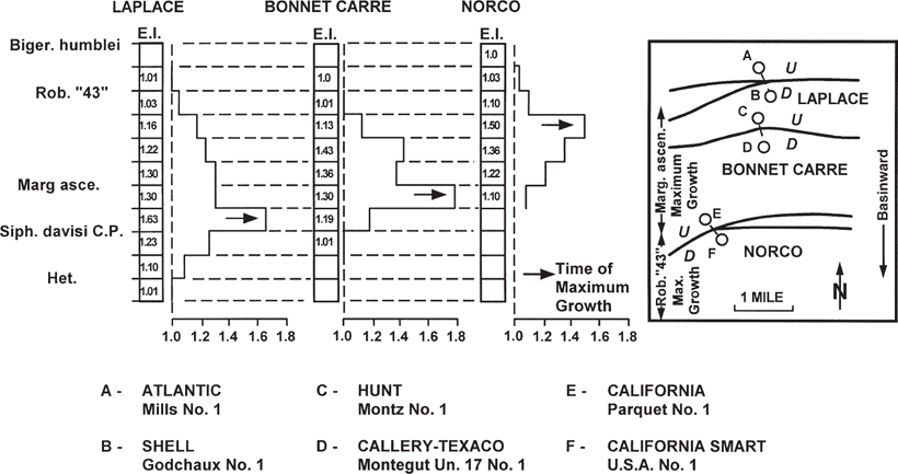
Figure 13-3 Expansion indices can be used to date growth faults with regard to their initial movement, time of maximum growth, and last movement. (From Thorsen 1963. Published by permission of the Gulf Coast Association of Geological Societies.)
The analysis of a growth fault, based on the pattern of its expansion indices, provides information important to the exploration for hydrocarbons. If time information is available, then at least eight benefits derive from analyzing the expansion index plot of a growth fault.
The plot shows the time of fault inception.
It indicates the time of maximum fault movement (maximum expansion).
It shows the time of cessation of fault movement.
It provides a complete history of fault movement.
Regionally, it can correlate stratigraphic units associated with maximum fault growth.
It can be used with structural growth indices to compare fault growth with structural growth of uplifted areas.
It can serve as a vertical correlation tool for seismic sections and well logs.
It serves as a lateral correlation tool for recognizing specific faults over long distances using well logs or separate seismic lines.
Some disadvantages to using the expansion index method are that, because it is a ratio, it has a low resolution and may contain mathematical ranges that can be significant (Bischke 1994b). In the next section, we describe the related, but high-resolution, Δd/d technique, also referred to as the Multiple Bischke Plot Analysis (MBPA). This technique minimizes mathematical ranges and errors, with maximum errors on the order of 0.1 percent (see Accuracy of Method section).
Multiple Bischke Plot Analysis and Δd/d Methods
Growth structures develop as sediments accumulate during tectonic events and sea level fluctuations, and they form coincident with faulting, subsidence, and diapirism. By analyzing the subsea depths of correlative horizons, we can glean information about sedimentary and tectonic history from the syntectonic sediments. Indeed, the geometry of a growth section contains the only records of the dynamic processes that are available to geoscientists. If we are to provide answers to tectonostratigraphic problems, then we must consult the growth section to decipher the details. In many areas, reliable correlation data exist to constrain interpretations, but the data may be ambiguous over problem intervals. These problem areas may result from facies changes, high bed dips, or rapidly thinning horizons. An analysis of the reliable portions of the growth section can help resolve practical problems that conventional methods, such as 3D seismic, cannot resolve.
In this section, we describe two methods for analyzing growth: the Δd/d method proposed by Bischke (1994b) and a related but more powerful method that Sanchez et al. (1997) and Chatellier and Porras (2001, 2004) call the Multiple Bischke Plot Analysis (MBPA). A single graphical plot of time-stratigraphic correlation markers forms the basis for the Δd/d method of growth analysis. Alternatively, MBPA is an enhanced graphical technique based on multiple Δd/d plots of correlation markers. Sanchez et al. (1997) show that comparing several Δd/d plots to each other often provides additional information for rapidly understanding the growth history or resolving problems related to growth.
These methods display, in graphical form, the growth history of a sedimentary section. Because the plots record changes in growth, the methods have a very high resolution, typically about one part in one thousand, when using well log correlations (Bischke 1994b). The technique appears capable on well log data of resolving subtle stratigraphic details that occur on sequence boundaries that have only several feet of missing section (see Accuracy of Method). On good-quality seismic profiles, the methods can identify disconformities having only 20 ft to 50 ft of missing section. The methods may help solve problems that result from changing sedimentary, eustatic, or tectonic conditions. These include (1) correlation problems in general and, specifically, on the flanks of salt bodies; (2) questions about fault timing and trapping of hydrocarbons; (3) locating subtle stratigraphic traps; and (4) identifying a variety of stratigraphic and structural problems not readily recognized by conventional interpretation techniques. The methods have application in all tectonic regimes, whether extensional, compressional, strike-slip, or diapiric. Geoscientists often encounter problems adjacent to salt diapirs if they cannot correlate well logs due to sands thinning dramatically toward or onto salt or to a thick multiple sand section, and they cannot correlate the seismic data because of poor imaging of high bed dips. In these situations, the MBPA method may be the only remaining avenue available to the solution of correlation problems. Furthermore, if correlation data is entered into a spreadsheet that contains a graphics program, then these methods can be very fast.
Growth can be recognized by a change in the true stratigraphic thickness of a unit within an area, and the Thorsen method calculates and compares thicknesses of a number of units. The MBPA method depicts growth by using a number of horizons and plotting the changes in depth of each horizon within an area. Unlike the Thorsen method, the interval thicknesses are not determined. Therefore, the MBPA method is easier to use, involves fewer measurement errors, and is more accurate. The method allows for the recognition of faults, unconformities, and incorrect correlations in the form of discontinuities, or anomalies, on the plots.
Method
In this section we describe the high-resolution Δd/d and MBPA methods and present a number of practical examples of these methods. The methods have application from the producing-field scale, with excellent well control, to the regional basin scale with minimal well control. We present several examples of salt-related problems that are not resolvable using conventional techniques, but are resolvable using growth plots. We first describe the Δd/d method, which is the foundation for MBPA.
To begin the method in an area of study, locate two wells in a general dip direction, so that one well is structurally higher than the other. Consider first a stable, or nongrowth, tectonic environment in which the correlative intervals between two wells have about the same thickness (Fig. 13-4a left). Correlative horizons are represented by correlative markers in the well logs. For simplicity in Figure 13-4a, the top correlative marker is at the same depth in both wells. The difference in depth of the lower marker reflects growth. Plot this depth difference (Δd) of each marker against its subsea true vertical depth (SSTVD) d in the structurally higher well (Fig. 13-4a right). In a stable tectonic environment, the slope on the Δd/d plot is approximately flat.
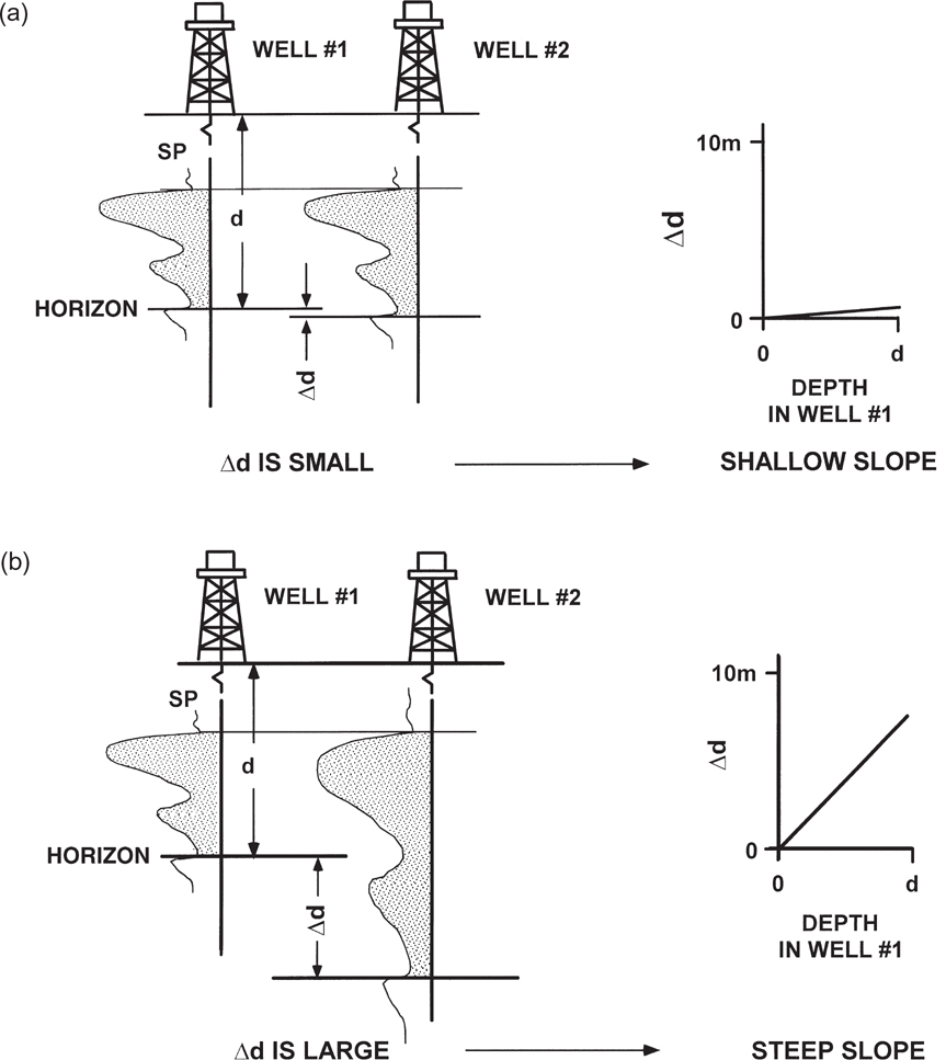
Figure 13-4 Sedimentary environments can be categorized into stable and unstable growth environments. (a) In a stable, nongrowth environment, the vertical distance between correlative markers is small. If the markers are plotted on Δd/d plots, then the curves will have a gentle slope. (b) In an unstable, growth environment, the vertical distance between correlative markers is large, and the resulting Δd/d curves are more steeply sloping. (Modified from Bischke 1994b, AAPG©1994. published by permission of the AAPG whose permission is required for further use.)
In an unstable, or growth, tectonic environment, differences in the thickness of correlative stratigraphic intervals are greater, and thus larger vertical distances (Δd) separate the horizons in the wells (Fig. 13-4b left). Typically, only two wells establish this relationship, although the wells need to be in the dip direction. The resulting Δd/d plot (Fig. 13-4b right) has a higher, or steeper, slope than the one for a stable environment.
Using a number of correlation markers generates more points for the Δd/d plot. The slope of the curve on the plot reflects the growth history of the interval plotted. In applying the technique, use many correlation markers that represent time-stratigraphic horizons. Such horizons include parasequence boundaries, which are valuable in MBPA. Determine the difference in depth of each marker in the pair of wells, and then generate a plot of the data. If you enter the subsea depths of the correlations in a spreadsheet, simply calculate the difference in depths of the correlations in the structurally higher well and those in the lower well to generate Δd values. Place the subsea depths of the markers in the higher well on the x-axis, and then plot the Δd value corresponding to each marker on the y-axis. This is best done in a spreadsheet program that contains a graphics package.
A pair of wells is always used in the analysis, but one of the wells can then be compared with a third well, a fourth well, and so on. This comparison forms the basis of the MBPA described in the next paragraph. A plot is generated for each pair of wells. To provide more analytical power to the method, when a given up-dip well is compared with a number of other wells, place all the plots generated on a single graph (Fig. 13-17b). This type of plot provides significant information on the overall area of study in terms of growth, faults, and unconformities. We provide several examples of the Δd/d analysis and MBPA later in this chapter.
When conducting an MBPA, compare a reference well to any number of adjacent wells by using a set of Δd/d plots of the reference well versus each of the other wells (Sanchez et al. 1997). The reference well on the cross plots could be a type well that has a complete stratigraphic section. Alternatively, the reference well can be any other well positioned on any structural level. Unlike the Δd/d method, plot the depths in the reference well on the x-axis, even though it may not be the structurally higher well. Thereby the reference well is present on all the plots.
The advent of 3D statistical programs enhances MBPA by allowing the comparison of a reference well to any number of other wells. The procedure rapidly generates Δd/d plots, printed on a single page. A visual comparison of these plots rapidly locates tectonostratigraphic anomalies. If the anomaly is present in the reference well, then the anomaly exists on all plots. However, if the anomaly is present in only one well, then the anomaly is in the well used for comparison, rather than in the reference well. This process allows interpreters to rapidly identify problem wells and to better understand the cause of the anomaly (Sanchez et al. 1997; Chatellier and Porras 2001).
Structural and stratigraphic analysis, based on comparison of Δd/d plots, can be enhanced if stratigraphic data are posted on the plots, as in Figures 13-14 and 13-17b. Then MBPA can be applied with respect to discrete stratigraphic intervals and thereby provide information directly relevant to the history of the study area.
Sanchez et al. (1997) describe their experience with previously correlated well logs. Should interpreters use pre-existing correlations, and perhaps be prejudiced by these correlations? Often this results in purely cosmetic changes to the correlations, adding little to the understanding of the field. A second, more time-consuming but more objective approach is to recorrelate the logs, ignoring the existing correlations. A third, less time-consuming approach is to subject the existing correlations to MBPA in order to rapidly identify correlation problem areas.
Consider the purchase of an older, producing field. The task at hand, besides producing the proven reserves, is to find any additional potential. How do we, as geoscientists and engineers, find additional potential in previously worked areas? New potential is found by disagreeing with, and changing, the previous correlations—in other words, finding error in the older work. We must remember that oil and gas reserves are not found by making maps. It is correlation work that identifies the potential, and then the mapping based on the correlations that graphically displays that potential.
If we take previous geoscience and engineering work, in the form of correlations of electric logs or correlations on seismic sections, and submit these correlations to a test of validity (MBPAs), we can rapidly identify problem correlations, previous correlation errors, faults and even unconformities. We can define the growth history of the area, providing us guidance as to the stratigraphic intervals that might hold the best potential for hydrocarbons. And most important, we can do this while reducing the cycle-time of the correlation and mapping process by as much as 50 percent (Bischke and Tearpock 1999).
This methodology should be applied to all correlation data sets during the initial stages of any project. Numerous field studies show that the MBPA method, when applied at the beginning of a study, results in a higher-quality product and can aid in the rapid identification of new hydrocarbon potential.
Common Extensional Growth Patterns
In extensional regimes, growth plots detect missing section due to normal faults or unconformities. The missing section occurs as discontinuities on the plots. In extensional regimes, three types of growth patterns commonly occur and can be used to interpret structural or stratigraphic history (Fig. 13-5).
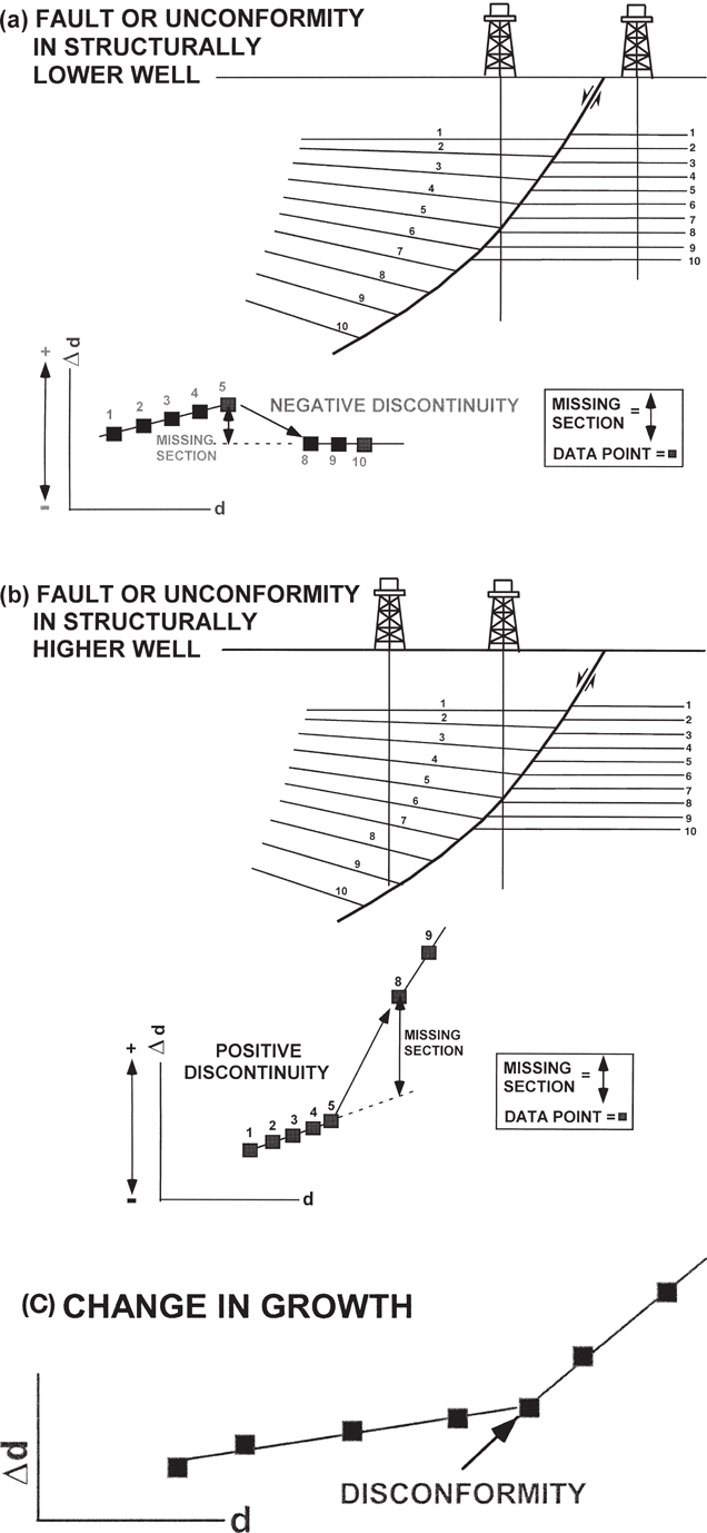
Figure 13-5 In extensional regimes, three patterns of discontinuities are observed on Δd/d plots. The discontinuities on the plots are caused by missing section that may be due to a fault or an unconformity. (a) If the missing section is in the structurally lower well, then the plot of Δd/d contains a negative, or downward, discontinuity. We use an example of a fault. (Published by permission of R. Bischke and D. Tearpock.) (b) If the missing section is in the structurally higher well, then the plot contains a positive, or upward discontinuity. We use an example of a fault. These patterns can help distinguish faults from unconformities in areas of high bed dip. (Published by permission of R. Bischke and D. Tearpock.) (c) A hiatus causes a change in slope on the plot. (From Bischke 1994b. AAPG©1994, published by permission of the AAPG whose permission is required for further use.)
Normal faulting typically results in missing section in correlated well logs. On the Δd/d plots, large faults produce large discontinuities, or offsets, in the plotted data, whereas small faults produce small offsets in the plots. If faulting is present, two types of patterns exist: a downward, or negative displacement pattern, in which Δd becomes smaller with increasing depth (Fig. 13-5a), and an upward, or positive displacement, in which Δd becomes larger with increasing depth (Fig. 13-5b). If a negative discontinuity is present, then the identified fault cuts the structurally lower well within the intervals being correlated (Fig. 13-5a). A positive displacement pattern means that the fault cuts the structurally higher well (Fig. 13-5b). Each of the faults in Figure 13-5a and b is interpreted as a growth fault because the growth rate is higher within the stratigraphic interval that is downthrown to the fault in the faulted well.
An unconformity is a surface of erosion and/or nondeposition caused by changing environmental conditions that affect growth. Erosion or downlap will create thickness changes within stratigraphic units. Unconformities, as do normal faults and sequence boundaries commonly, eliminate stratigraphic section and produce missing section in correlated logs, and so they generate discontinuity patterns on the growth plots. Thus, large unconformities resemble faults. As a rule, however, unconformities tend to remain at or near the same stratigraphic level over large areas and in many wells. Geologists recognize that normal faults usually dip at high angles of 40 deg to 60 deg (Ocamb 1961) and that a fault intersects different wells at different stratigraphic levels. An unconformity, however, if it covers a large area, appears at about the same stratigraphic level in the wells in the area and typically dips at a lower angle. For example, a so-called fault, interpreted to be the cause of the same stratigraphic section missing in many wells in a study area, actually would be an unconformity rather than a fault. The existence of missing section at the same stratigraphic level is obvious on a set of Δd/d plots. Accordingly, geoscientists employ the method to rapidly locate unconformities and to rapidly distinguish faults from unconformities in well log data. If many wells exist in an area of study, then the plots aid in keeping track of the missing section and its approximate value and stratigraphic level in each well (Fig. 13-17b). The plots represent a record of the missing section in the form of a visual display that is readily apparent. Refer to Figure 13-17b and review Fault J and the recognized unconformity.
Often a more difficult problem develops for geoscientists where structure was growing very slowly relative to changing sedimentation rates or where sedimentation rates were high relative to deformation rates. In these cases, it is difficult to detect disconformities in well log data, and downlap may not be obvious or present on seismic sections. If there were a hiatus in deposition (a condensed section), then when sedimentation resumes, the rate of deposition would likely change. Tobias (1990) stresses this point. Subtle unconformities, caused by gradual processes, occur as changes in slope of the Δd/d curves (Fig. 13-5c). Alternatively, if there is the slightest change in the sedimentation rate, regardless of its cause (e.g., sea level fluctuations), then changing environmental conditions are likely to produce changes in the slope of a Δd/d curve displayed on the plot. These plots are very sensitive to changes in the tectonically or eustatically controlled sedimentation rate, so disconformities and/or subtle sequence boundaries commonly occur as breaks in slope of the curves generated on the Δd/d plots (Fig. 13-5c).
Unconformity Patterns
Two unconformity growth patterns exist, one for onlap and the other for downlap. These patterns may help define systems tract boundaries.
If beds onlap an unconformity, then at the time of deposition the beds above the unconformity dip at a lower angle than the beds below the unconformity. Figure 13-6a shows the typical occurrence of onlap above an unconformity, with the missing section being greater in the well located at the structurally higher position at the time of deposition. Erosion typically removes more section in the up-dip direction than in the down-dip direction. The missing section caused by the unconformity occurs as a positive displacement on the Δd/d plot (Fig. 13-6a), even if strata were later structurally rotated. Thus, if a positive discontinuity is present on a Δd/d plot (Fig. 13-5b), the missing section results either from a fault in the structurally higher well or from erosion, with subsequent onlap of sediments above the unconformity.
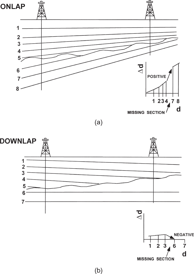
Figure 13-6 (a) Onlap produces a positive discontinuity on the Δd/d plot, whereas (b) downlap creates a negative discontinuity. (From Bischke 1994b; AAPG©1994. Published by permission of the AAPG whose permission is required for further use.)
If beds downlap an unconformity, then at the time of deposition, the beds above the unconformity dipped at a higher angle than the beds below the unconformity. Downlap causes a negative discontinuity on Δd/d plots (Fig. 13-6b), even if strata were structurally rotated. Again, more section is missing in the area that was up-structure at the time of deposition. Thus, if a negative discontinuity exists on a plot, then the missing section responsible for the discontinuity results either from a fault in the structurally lower well or from erosion, with subsequent downlap of sediments above the unconformity.
These patterns enable us to distinguish faults from unconformities on the steeply dipping flanks of salt structures, where bed dips are commonly too steep to image on seismic data. For example, on the flanks of salt diapirs the sedimentary units typically onlap, rather than downlap, an unconformity. Therefore, unconformities on the flanks of salt domes produce positive, rather than negative, discontinuity patterns (Fig. 13-6a). This concept can be used in comparing an up-dip well to one or more structurally lower wells. If missing section causes a negative displacement on the plots, as shown in Figure 13-5a, then the missing section in the structurally lower well must be due to a fault rather than to an unconformity.
The larger the missing section, the larger the discontinuity in the Δd/d plots. However, consider that an unconformity removes section in both of the wells used in a Δd/d plot (Fig. 13-6). Then the amount of missing section, estimated from that plot, is the difference between the amounts of the two missing sections, rather than the actual amount of section missing in one of the wells.
Accuracy of Method
Well log data has a higher resolution than 3D seismic data. At a depth of −15,000 ft, geologists can commonly determine the depths between two correlation markers to within a few feet (e.g., 5 ft). A Δd/d plot is a plot of change-in-depth versus total depth. Therefore, if we define error as the precision in correlation between two tops, divided by the subsea depths to the correlations, then the error in well log data at −15,000 ft is 5/15,000, or 1 part in 3,000 (0.03%). This is a very high degree of accuracy. Thus, Δd/d plots constructed from well log data typically have errors on the order of less than 0.1%.
Seismic data at a depth of −15,000 ft may have a velocity of about 10,000 ft/sec one-way time, and a frequency of 30 Hz. These data would have a wavelength of about 500 ft and a resolution of about 100 ft (Sheriff 1980). At a depth of −15,000 ft, seismic data has an error of 100/15,000, or about 1 part in 150, or about 0.7%. Well log data are at least one order of magnitude more precise than seismic data. The intent of this discussion is not to degrade seismic data that we use on a daily basis but rather to point out the accuracy of the methods when using well log versus seismic data.
The plots will contain errors in the slope of the growth curves if a well encounters changes in bed dips or changes in wellbore deviation angle (Chatellier and Porras 2001). This error affects only the slope of the growth curves, and the error increases as the tangent of the change in bed dip angle or wellbore deviation angle (Bischke 1994b). The plots of (1) vertical wells against the ramp portion of deviated wells or (2) two subparallel deviated wells, compared to each other, contain fewer errors than plots based on highly deviated wells and horizontal wells, and these latter types of plots should be avoided. Thus, during correlation work, if vertical wells, the ramp portion of deviated wells, or two subparallel deviated wells are available for study, then it is generally not necessary to correct the data. If, however, the intent of the study is to distinguish high-growth intervals from low-growth intervals, and the dipmeter data indicate rapidly changing bed dips, then the data can be corrected for changing bed dips by using the correction factors presented by Bischke (1994b). The errors present in uncorrected data accumulate as the tangent of the change in bed dip angle; for example, if the bed dip changes by 10 degrees, then the error introduced in the slope of the curves is 18%.
Examples of the Δd/d Method
Generic Example of a Delta
In order to understand the application of Δd/d plots and Multiple Bischke Plots, let’s review a generic example prior to discussing practical examples of the two methods. We use a generic delta that contains six parasequences to demonstrate how the technique works (Fig. 13-7). The stratigraphic intervals between horizons 3 and 6 are of constant thickness, so these units represent a nongrowth section. These units downwarp with the deposition of prograding units, between horizons 0 and 3, upon the older sequences. For this example, we study three wells advantageously positioned on the delta (Fig. 13-7).

Figure 13-7 Stratigraphic interpretation of a generic delta based on well control. Parasequence correlations define a nongrowth (pregrowth) section in the wells beneath a disconformity located at correlative horizon 3. Growth section above the disconformity contains an expanded section between Wells No. 1 and 2, and a condensed section between Wells No. 2 and 3. Expanded and condensed sections are characteristic of wells located across a delta, and thus the method may define sedimentary environments in areas that lack dense well control. A seismic line located between Wells No. 1 and 3 would not detect the hiatus. (From Bischke 1994b. AAPG©1994, published by permission of the AAPG whose permission is required for further use.)
From the correlation data obtained from the wells, we construct two Δd/d plots in the form of bar graphs. We generate the data by correlating the logs and noting depth differences for each correlation marker, as illustrated in Figure 13-7, by drawing a horizontal dashed line between the wells for each correlation marker. Horizontal lines are drawn between Wells No. 1 and 2 to illustrate the depth of correlation markers 1 through 6 in Well No. 1. Measure the vertical distance (difference in depth) for each of the correlative markers, 1 through 6, in each pair of wells. Plot these Δd values on the y-axis against the subsea depth of the correlations in the structurally higher well, plotted on the x-axis (Fig. 13-7). In practice, calculate the Δd measurements on a spreadsheet by entering the subsea depths as positive values and subtracting the depths in the structurally higher well from the depths in the structurally lower well. The plot for Wells No. 1 and 2 are shown in Figure 13-7. These data can be from anywhere in the world and from any tectonostratigraphic environment, yet the following interpretation will be correct.
The interval between correlations 1 to 3 is an expanded, growth interval, and the interval between correlations 3 through 6 is a nongrowth interval. We can see that the interval 1 to 3 has a positive slope on the plot, demonstrating expansion from Well No. 1 toward Well No. 2. The slope is flat between correlations 3 through 6, indicating no growth. As no onlap is present, the break in slope at correlation 3 is a possible disconformity that would not image on seismic profiles between Wells No. 1 and 2.
To continue the analysis, we conduct the same procedure between Wells No. 2 and 3. In this case, a sequence boundary, labeled 0, is present in the two wells (Fig. 13-7). Again, a Δd/d plot shows the growth history relative to the two wells. Well No. 2 is the structurally higher well, so it is plotted on the x-axis (Fig. 13-7).
A unique interpretation of the plot of Wells No. 2 and 3 is made. The interval between correlations 1 and 3 is a condensed section in Well No. 3, and the interval between correlations 3 through 6 is a nongrowth interval. The interval 1 to 3 has a negative slope, which means that the section thins from Well No. 2 toward Well No. 3, indicating a condensed section in Well No. 3. The slope is flat between markers 3 through 6, confirming the nongrowth interval. The break in slope at correlation 3 is probably a time-transgressive disconformity that exists in all three wells. We can now conclude that the growth section expands between Wells No. 1 and 2 and contracts between Wells No. 2 and 3, which is characteristic of only a few sedimentary environments, including a delta. When integrated with other geological information, the technique can identify or constrain the number of possible structural styles or sedimentary environments in the area of study, even where data are limited.
Applying the Δd/d Method to Seismic Data
We can construct Δd/d plots from either well logs or depth-converted seismic sections. As discussed previously, the seismic sections used must be depth-converted, since time distorts vertical distance on seismic sections. The entire section need not be depth-converted. As long as we have reasonable time–depth data, the correlation markers picked in time from the section can be converted to depth before input of the data into a Δd/d plot.
For this example, we use a seismic section (Fig. 13-8a) from the offshore Gulf of Mexico, across the area called the Brazos Ridge. The seismic profile illustrates a large, listric growth fault, which nearly flattens with depth. A faulted rollover anticline exists in the hanging wall block. The hanging wall anticline has one master synthetic fault, several downward-dying synthetic faults, and a number of downward-dying antithetic faults.

Figure 13-8 (a) Seismic section in the Brazos Ridge area, northern Gulf of Mexico. Inclined dashed lines are locations for correlation data in a Δd/d plot. (b) A Δd/d plot of data, derived from (a), reflects changes in growth history of the structure. The breaks in slope, at data points 8, 12, 18, and 22, mark major sequence boundaries. (Bischke 1994; AAPG©1994 reprinted by permission of the AAPG whose permission is required for further use.)
In this example, we use the correlated seismic data between the two major synthetic faults to look for unconformities or sequence boundaries and to help us understand the growth history of the area. The Δd/d plots, which record changes in the sedimentation rate, are very sensitive to changing structural and sedimentary conditions.
The two dashed lines between sp C and sp D define the area used to obtain the data for analysis. Since this area is free of any visible faults, the resulting plot will not be complicated with fault patterns. The two dashed lines can be considered for simplicity as two fictitious directionally drilled wells. These dashed lines are essentially parallel to each other and to the bounding faults. We can obtain correlation data on each event that has been correlated on the seismic section. The more events (markers) correlated, the better the results.
By observation of this single seismic section, can you see the sequence boundaries? Can you see an angular unconformity that might set up traps? Can you visualize the growth history of this area? Most likely, the answer to each question is no. However, once we subject the correlation data to Δd/d analysis, the questions should be easily answered.
Figure 13-8b is the Δd/d plot generated from the correlation data obtained from interpretations of the seismic section. More than 26 markers were correlated in the master synthetic fault block (Fig. 13-8a) and carried through the two dashed lines. Since the beds dip into the fault near sp C, the correlation data obtained from the dashed line near sp D is considered as the data that would be equivalent to that obtained from a higher structural well (it is in the higher structural position). The correlation data, which are in time, are first depth-converted using local time–depth information, and then plotted as shown in Figure 13-8b.
We see various changes in the growth history of the area and at least five distinctive changes in the slope of the plotted data. The plot illustrates at least four major breaks in the growth trends, from a condensed section between Δd/d points 22 to 26 to a nongrowth section above −1000 ft. The maximum growth occurred in this area between correlation points 12 and 18. And finally, the breaks at correlation points 8, 12, 18, and 22 appear to mark major sequence boundaries.
This one Δd/d plot, from one seismic section from a 3D seismic survey, provides significant information about the stratigraphic and growth history of this area of the Brazos Ridge. Plots from other seismic sections also exist. The combined use of multiple Δd/d plots, using seismic sections like the one shown in Figure 13-8a, provide significant information on the tectonostratigraphic history of an area and begin to define its hydrocarbons potential.
Resolving a Log Correlation Problem
We now turn to an example of the Δd/d method and consider how it aids in the resolution of difficult correlations. Such difficulties are common between on-structure and off-structure wells in complex tectonic settings, such as diapiric areas. The first example is from the northern Gulf of Mexico, offshore USA. Well No. 1 is on top of a salt dome, and it has a section that is difficult to correlate between 7000 ft and 9000 ft. 3D seismic data are incoherent in this area.
We begin by successfully correlating an off-structure type well (Well No. 5) with several surrounding wells, as well as with up-dip wells. Based on these correlations, the off-structure type log of Well No. 5 has a complete stratigraphic section. We then correlate Well No. 5 with the problem Well No. 1 on top of the salt diapir. A total of 31 parasequence boundaries are correlated between the two wells, resulting in the Δd/d plot shown in Figure 13-9a. Notice that the x-axis has an expanded scale relative to the y-axis, which is typical for Δd/d plots.

Figure 13-9 (a) Growth plot of the type Well No. 5 and the difficult-to-correlate Well No. 1 in the Eugene Island 208/215 field. Correlation marker No. 27 lies 230 ft off the general growth trend, suggesting that this anomaly is due to miscorrelation or to faults in the two wells. See text for explanation that marker No. 27 in Well No. 1 is miscorrelated to the type log by about 230 ft. (b) The 8600-ft sand in Well No. 5 was initially incorrectly correlated to the 7800-ft sand in Well No. 1. The Δd/d method, when integrated with other geological information, demonstrates that the 8600-ft sand in Well No. 5 correlates to the sand below 8000 ft in Well No. 1. (From Bischke et al. 1999. Published by permission of the Gulf Coast Association of Geological Societies.)
Although Wells No. 1 and 5 are not close to each other, the growth plot shows near-linear growth through the entire 9000-ft section. Notice on Figure 13-9a that parasequence boundary correlation No. 27, located in the difficult-to-correlate portion of Well No. 1, lies about 230 ft off the general linear trend. This data point is based on the initial correlation shown in Figure 13-9b.
Two possible interpretations of the data are (1) a miscorrelation exists in Well No. 1 as correlated with Well No. 5, and correlation marker No. 27 is about 230 ft too high; or (2) the anomalous correlation marker No. 27 is, by coincidence, faulted up in Well No. 1 by 230 ft relative to Well No. 5, and then faulted down in Well No. 5 by the same amount. By comparison to Figure 13-5a, the possible 230-ft fault, responsible for down-faulting correlation marker No. 27, must exist in the off-structure Well No. 5 (at about the 8600-ft level). However, correlation with wells adjacent to Well No. 5, together with the 3D seismic data, indicate that Well No. 5 does not penetrate a 230-ft fault near the 8600-ft level. Therefore, interpretation (2) cannot be correct. So a miscorrelation exists in Well No. 1.
Notice on Figure 13-9b that another possible correlation to the 8600-ft sand in Type Well No. 5 exists below the 8000-ft level in Well No. 1. This sand is about 230 ft deeper than the initial correlation at 7800 ft in Well No. 1. The Δd/d method, when integrated with the existing geological information, strongly suggests that the lower sand correlation, below 8000 ft, is the correct correlation. This change in correlation affects the interpretation, including the fault pattern, reservoir delineations, volumetrics, and additional potential production.
When used in conjunction with other geological information, the Δd/d method may “uniquely” resolve correlation problems. The method also determines whether correlations of horizons are either too high or too low, and it specifies the approximate vertical distance between the correct and incorrect correlation picks. In Figure 13-9, this vertical distance is 230 ft. The method is most useful in areas where reliable correlation data exists but nevertheless the data deteriorate within a problem interval. This commonly occurs around salt diapirs or on other structural features that exhibit steep bed dips, such as compressional structures. If a near-linear growth trend is identifiable on the plot, then the method directs the interpreter to an alternative correlation. The method uses a nonarbitrary process.
An Example of Stratigraphic Interpretation
The Δd/d method is capable of locating disconformities and hiatuses from well log data and on seismic profiles, along with associated sequence boundaries (Fig. 13-8). In this section, we show how the method can distinguish between lithostratigraphic units and genetically related stratigraphic units, which may aid in locating sequence boundaries.
The example is from a carbonate section in the Guadalupe Mountains, New Mexico, USA (Fig. 13-10). The Grayburg Formation formed in a shallow marine-to-supertidal environment within a sigmoidally shaped carbonate ramp that contains fifth-order parasequences that shallow upward (Lindsay 1991). The Grayburg Formation is subdivided into five stratigraphic units called zones. The overlying Queen Formation contains shallow marine sandstones, carbonates, and evaporites (Vanderhill 1991). Kerans and Nance (1991) interpret the Grayburg Formation to be in the high stand systems tract (HST) below a probable Type 1 sequence boundary. They conclude that the base of the Queen Formation reflects a rise in sea level.
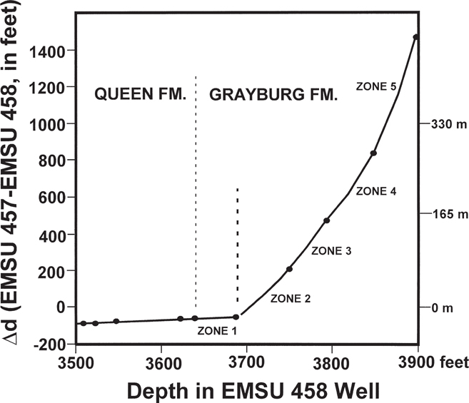
Figure 13-10 Growth plot illustrating carbonate ramp in Grayburg formation, Guadalupe Mountains, New Mexico, USA. The change in slope at the top of Zone 2 partitions the Grayburg Formation into high-growth and low-growth sequences, and indicates a probable tectonostratigraphic boundary. A genetic relationship exists between Zone 1 in the Grayburg Formation and the overlying Queen Formation. (Published by permission of R. Bischke.)
Using core and well log correlations from Lindsay (1991), we generate a growth plot from Wells No. EMSU 458 and 457 (Fig. 13-10). The data points include the tops of Lindsay’s Zones 1 to 5 within the Grayburg Formation and tops of several parasequences in the Queen Formation. Zone 1, at the top of the Grayburg Formation, is within a low-growth section (Fig. 13-10). This linear low-growth pattern continues into the Queen Formation, and thus Zone 1, in the Grayburg Formation, appears to be genetically related to the Queen Formation. Contrastingly, a high-growth section is seen in Zones 2 through 5. Growth rate was highest during deposition of Zone 5, then gradually declined through Zone 2. Zones 2 to 5 in the Grayburg Formation define the carbonate ramp.
A disconformity appears to exist at the top of Zone 2 within the Grayburg Formation (compare Figs. 13-5c and 13-10). We interpret this hiatus to result from a change in sea level. The growth plot, constructed from correlations based on well log and core data, is compatible with a genetically related boundary at, or very near, the top of Zone 2 in the Grayburg Formation. Zone 1 in the Grayburg is genetically related to the Queen Formation. A Δd/d plot of Wells EMSU 458 and 247, not shown in this book, yields similar results with the carbonate ramp represented beneath the top of Zone 2. If sedimentary sequences exist as genetically related units, regardless of the cause, then these units are likely to be related to sediment supply. Changes in sediment supply should occur at or near system tract boundaries, where changes in sea level affect growth. We conclude that changes in growth may occur at, or near, major sequence boundaries and may aid in locating the position of sequence boundaries (Tobias 1990; Sanchez et al. 1997). The method can help distinguish between lithostratigraphic and tectonostratigraphic boundaries.
Locating Sequence Boundaries in a Compressional Growth Structure
The Newport-Inglewood Trend, in the western Los Angeles Basin, California, USA (Harding 1973; Wright 1991), is a classic zone of compressive and strike-slip deformation that involves growth. Producing fields exist in folds within the trend, and the trend was mapped by the California Division of Oil and Gas beginning in the late 1920s. The Division geologists typically mapped the unconformities and were able to carry the upper and lower Pliocene and Miocene sequence boundaries from growth fold to growth fold.
Growth plots that we made support the ability to correlate sequence boundaries between fields. As an example, Figure 13-11 shows a Δd/d plot for the Huntington Beach Field Anticline, located in the southern part of the Newport-Inglewood Trend. The plot uses data from an off-structure well and a well located near the crest of structure, as presented by Harding (1973). The plot consists of near-linear increments of growth punctuated by discontinuities. Correlation to adjoining wells shows that the wells are not faulted, so these discontinuities represent missing section due to disconformities. These disconformities represent several tens of feet of missing section and are regional time-stratigraphic boundaries (Wright 1991; Blake 1991). The hiatus at point 1 is near the top of the Pliocene, and the Top Reppeto, at point 2, is a late Pliocene sequence boundary in the Huntington Beach Field Anticline. Points 4 and 5 are early Pliocene and Top Miocene sequence boundaries. The California Division of Oil and Gas mapped every disconformity except the anomaly at point 3, and were thus able to readily correlate between adjoining fields. The California Division of Oil and Gas recognized the value of sequence stratigraphy in the late 1920s.
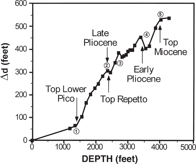
Figure 13-11 Growth plot for Huntington Beach Field Anticline, Newport-Inglewood Trend, California, USA. The compressional fold grew during the Pliocene. The highest growth interval is between the Top Repetto and Top Lower Pico section. Disconformities exist at discontinuities on the plot, indicated by the circled numbers. The California Division of Oil and Gas mapped these disconformities between fields in the Newport-Inglewood Trend.
The slopes on the plot indicate intervals of growth of the Huntington Beach Anticline, which may have implications concerning hydrocarbon generation and migration. This anticline grew during the Pliocene (Fig. 13-11). If hydrocarbon generation and migration occurred before the Pliocene, then there was no structure to trap the hydrocarbons. The low-growth interval, shallower than point 1 on the plot, represents the onlap of the Pleistocene Pico Formation across the crest of the anticline. These Pleistocene sediments are cut by the Inglewood Fault System and were not subject to folding (Harding 1973). The conclusion is that the migration of hydrocarbons into the Huntington Beach Anticline was post-Miocene.
Lastly, the plot helps to interpret the structural style. The Newport-Inglewood Trend is subject to several interpretations. Harding (1973) proposes that strike-slip displacements caused, and were coincident with, the compressional folding. Wright (1991) employs structural maps and well log data from fields along the trend to conclude that the folding and faulting exhibit a complex structural and stratigraphic history, not readily reconciled with a simple strike-slip origin. From a seismic study of the Los Angeles Basin, Shaw and Suppe (1996) conclude that the Los Angeles Basin is subject to large-scale, blind-thrust faulting, and that the folding is not coeval with recent strike-slip displacements on the Newport-Inglewood fault system. Thus different interpretations are possible for the structural formation of the local folds. Which is correct? Can the growth plot suggest the correct solution? The Δd/d plot seems to support the interpretation of Shaw and Suppe (1996). In the same Newport-Inglewood trend, a study of several growth plots and a restoration of the Signal Hill restraining bend, at the Long Beach Anticline, provide evidence that the strike-slip faulting postdates the compressional folding. The Signal Hill analysis is presented in Chapter 12.
A Δd/d plot of the correlations presented in Harding (1973), when integrated with the local geological data (Wright 1991), suggests that the Huntington Beach field is a growth anticline (Fig. 13-11). A growth compressional style may be new to many geoscientists and engineers alike. A lack of knowledge of growth compressional structures can cause misinterpretations that may affect regional interpretations, the interpretation of the local petroleum system, and ultimately the prospects generated. Any interpretation based on existing correlations must be consistent with the correlations, regardless of the structural style under study.
Analysis of the Timing of a Strike-Slip Growth Structure
The Δd/d method can be applied to strike-slip faults as well, whereby we can determine when a strike-slip fault was active. This information may provide support as to when the fault system provided a hydrocarbon conduit into associated structures. Many strike-slip faults cut through the sedimentary cover into basement (Harding 1990), and thus some strike-slip faults may tap deep source rocks. Motion on active strike-slip faults may create deep conduits for hydrocarbons, particularly at extensional, releasing bends (Chapter 12). Therefore, active strike-slip faults may have a greater potential for hydrocarbon accumulation in associated traps, than inactive faults. In addition, the trapping structures along strike-slip faults must exist prior to the migration of hydrocarbons along the nearly vertical fault surfaces.
The Δd/d plots have application for determining the growth history of strike-slip displacements. Contrary to intuition, the Δd/d method applies also to faults that exhibit predominantly horizontal displacements, for several reasons. First, prior to the movement along the fault, the area affected by the later strike-slip faulting may contain paleogeographic or paleobathymetric relief. Once the motion on the fault commences, the nonuniform topographic relief may lead to progressive juxtaposition of topographic highs against lows. Growth sediments deposited across the paleosurfaces are thinner across the highs and thicker across the lows.
Most strike-slip faults contain components of dip-slip displacements, and growth sedimentation may occur across the faults during fault activity. The Δd/d plots readily record the dip-slip component of growth in the same manner as recorded across growth normal faults. The assumption is that the dip-slip component of displacement correlates to the strike-slip component of displacement. However, a dip-slip component of motion need not accompany every strike-slip component of motion. The Δd/d method cannot distinguish between horizontal and dip-slip motions. Chapter 12 presents methods for recognizing horizontal displacements.
As an example of strike-slip fault analysis, we use the Zayante Fault, a large fault located about 5 km south of the surface trace of the San Andreas Fault in southern California (Clark and Reitman 1973). Deformed Pliocene and Quaternary sediments along the fault suggest recent activity on the Zayante Fault. We apply the Δd/d plot to wells separated by a splay of the Zayante Fault in order to determine when the fault was active (Shaw et al. 1994).
We select two wells for studying displacements on the Zayante Fault, and the two well locations are shown on the map in Chapter 12, Figure 12-17. The structurally higher Pierce Well is about 2 km to the south of the fault zone. The Light Well is the structurally lower well, and it is located northeast of the Pierce Well and on the opposite side of a splay off the main Zayante Fault (Shaw et al. 1994). The Light Well contains a thicker stratigraphic section than the Pierce Well, and the thicker section is shown to be a growth section by Δd/d analysis. Sixteen parasequence boundaries were correlated within the Pliocene and Pleistocene sections of the two wells. The Δd/d plot in Figure 13-12, generated from Pierce and Light well log data, shows that growth initiated in the section between the deposition of parasequence boundaries 5 and 6 (late Pliocene). The plot exhibits a pregrowth, or low-growth, interval below 200 m. Between parasequence boundaries 1 and 5, the stratigraphic interval continues to expand into the Pleistocene section. This linear expansion continues into the Recent, as evidenced by offset alluvial terraces (Fig. 13-12). Thus, displacements on the splay of the Zayante Fault began in the late Pliocene, between parasequence boundaries 5 and 6, and continued into the Recent, as evidenced by the offset terraces (Fig. 13-12). Other Δd/d plots from the area show similar growth histories on different splays of the Zayante Fault. Therefore, in some cases Δd/d plots can detect time of movement on strike-slip faults. If hydrocarbon migration occurred within the fault zones during periods of movement, the Δd/d analysis of fault timing provides valuable information regarding petroleum potential. The structures formed by movement on the fault(s) would necessarily predate hydrocarbon migration in order for accumulation to occur.

Figure 13-12 Growth plot for a splay of the Zayante Fault, California. Growth began between the deposition of parasequence boundary correlations 5 and 6 in the late Pliocene. Growth continues into the Recent, as evidenced by offset terraces. (From Shaw et al. 1994. Published by permission of the United States Geological Survey.)
The Multiple Bischke Plot Analysis
Sanchez et al. (1997) developed a significant enhancement to the Δd/d method. They use well log data from Venezuela to generate multiple cross-plots of correlation data, using the Δd/d method. They call this multiple well log correlation technique the Multiple Bischke Plot Analysis (MBPA).
The MBPA can be more powerful than that of a single Δd/d plot. First, the method compares many wells to each other, increasing the probability that an anomalous correlation marker in a problem well will not be overlooked. Second, a quick perusal of several Δd/d plots may rapidly direct geoscientists to the well that contains an anomalous correlation marker or problem. Additional well log correlation or seismic analysis can then be directed at the anomalous correlation to rapidly identify the cause of the anomaly. MBPA is versatile and does not require knowledge of which well is in the structurally higher position. The wells can be in any structural position and can even be along strike. Lastly, different types of plots can be constructed to emphasize or to demonstrate a concept or observation. Several Δd/d plots, all using the same reference well, can be grouped on a single plot to form a stacked Multiple Bischke Plot (Chatellier and Porras 2001). Stacked MBPs allow geoscientists to compare thickness changes between wells, or to locate an anomaly or missing section that exists in every well. As an example of a stacked MBP, see Fig 13-17b.
Another type of analysis is the inverted MBP (Chatellier and Porras 2001). For this analysis, the axes on the standard Δd plot are inverted, with Δd plotted on the x-axis and d plotted on the y-axis. Inverted MBPs contain properties similar to conventional stratigraphic cross sections, in that the y-axis values correspond to different depths in a reference well. These plots help to identify decollement levels and stratigraphic intervals that are partially faulted out of wells (Chatellier and Porras 2001, 2004).
In the format presented by Sanchez et al. (1997), MBPA is based on three or four Δd/d plots placed on a single page. Common to all these Δd/d plots is the same reference well. On the left side of each of the plots is the number of the reference well (top number), along with the number of the well used for comparison (bottom number), as in (Fig. 13-13). The Δd values are on the y-axis, but in this case, the depths in the reference well are on the x-axis, regardless of its structural position relative to the comparison well. Thus, the reference well is present on all the plots.

Figure 13-13 Definitions for a Multiple Bischke Plot. The comparison of a reference well (top number on left), with depths plotted on the x-axis, to a comparison well (bottom number on left), forms the basis for the Multiple Bischke Plots. Unlike the Δd/d method, the reference well can be on any structural level and need not be the structurally higher well.
MBPA to Recognize Correlation Problems
Using an example from eastern Venezuela, we employ MBPA to locate an interpretation anomaly that is due to a miscorrelation in a particular well. Figure 13-14 is Multiple Bischke Plot showing a stratigraphic miscorrelation from a producing field in eastern Venezuela (Sanchez et al. 1997, Chatellier and Porras, 2004). The correlation data points on the plots are flooding surfaces interpreted from the field data. The numbers C4 through C7 represent productive units within the field. The Multiple Bischke Plots compare Wells No. 485, 910, and 834 to reference Well No. 365. The vertical lines on the plots indicate known faults. Notice on all three plots that a correlation point for a flooding surface within the C6 unit lies about 70 ft below the straight-line portion of the curves (see arrows). As this anomaly exists on all three plots, the authors attribute the anomaly to a miscorrelation in reference Well No. 365.
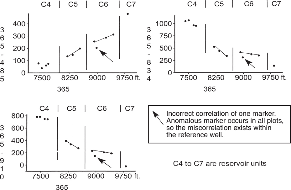
Figure 13-14 A Multiple Bischke Plot of flooding surfaces from a field in Venezuela. Anomalous point in the C6 unit, in all plots, suggests a possible stratigraphic miscorrelation in the reference well (From Sanchez et al. 1997. Published by permission of Latinoamericano de Sedimentologia, Sociedad Venezolana de Geologos.)
The next example is from a salt-cored structure and involves a well that bottoms in salt near the crest of the structure (Bischke et al. 1999). Steep bed dips caused the 3D seismic data to become incoherent, and a rapidly thinning stratigraphic section on the flanks of the dome caused reduced confidence in the well log correlations. The 3D seismic data were tied to off-structure wells. The initial mapping, based on a computer-mapping program, indicated that two horizons crossed each other in the up-dip direction, near the top of salt, which is impossible (Fig. 13-15). How do you resolve a mapping and correlation problem if you cannot correlate the 3D seismic data or the well logs with confidence?
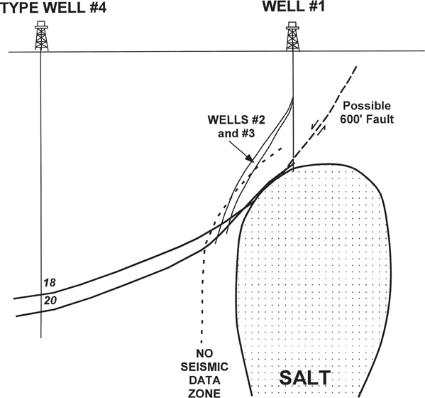
Figure 13-15 High bed dips on the flanks of diapirs may cause 3D seismic data to deteriorate, as in this example. Inability to correlate the well logs may result in incorrectly correlated horizons in the structurally higher wells. A projection, by a mapping program, of the 18 and 20 Horizons up-dip into the no-seismic-data zone caused the 18 and 20 Horizons to cross, which is impossible. MBPA provides the means to resolve the structural and stratigraphic problems.
The high bed dips and a rapidly thinning stratigraphic section along the flank of the diapir and near Wells No. 1, 2, and 3 made the seismic and well log correlations inconclusive (Fig. 13-15). A three-point problem, constructed from other wells that flank the diapir, results in an average bed dip of 42 deg. Higher bed dips are likely to be encountered up-dip, as the strata conform to the salt face. Best-guess correlations of the well log data resulted in an inaccurate pick for what is called the 20 Horizon in the up-dip Well No. 1. Seismic picks were tied to the well control and maps were generated. The computer-mapping program projected mapping horizons into the area of incoherent seismic data. The result was that the deeper 20 Horizon crosses the shallower 18 Horizon up-dip of Wells No. 2 and 3. This is impossible. There is a significant distance between where the seismic data deteriorate and where the log data for Wells No. 1, 2, and 3 are used to generate ties to the seismic data, which were used in the final interpretation and maps.
Recognizing the problem, a solution must be determined. There are three questions to answer: (1) Is the 20 Horizon correlated too high, or is the 18 Horizon correlated too low? (2) Could there be unrecognized faulting that is not imaged in the 3D data set? (3) What does one do when both the seismic and well log data cannot be correlated with confidence? When confronted with difficult problems of this kind, the MBPA may converge on a viable structural solution to the problem (Bischke et al. 1999). Given their associated correlation problems, we want to compare Well No. 1 with nearby Wells No. 2 and 3. These wells are down-dip of Well No. 1, have thicker stratigraphic sections, are close to each other, and are easier to correlate than Well No. 1.
When using MBPA, experience has shown that comparing wells that have correlation problems to a type well can help resolve those problems. Wells No. 1, 2, and 3 are compared to a reference Well No. 4, which is an off-structure well. Figure 13-16a and b are two Δd/d plots constructed for Wells No. 2 and 3, using Well No. 4 as the reference well. These two plots indicate that the growth rate gradually increases from the 1 Horizon down through the 20 Horizon in both Wells No. 2 and 3. Gradual (monotonic) changes in growth on Δd/d plots are a common pattern observed in different tectonic environments (Bischke 1994b).
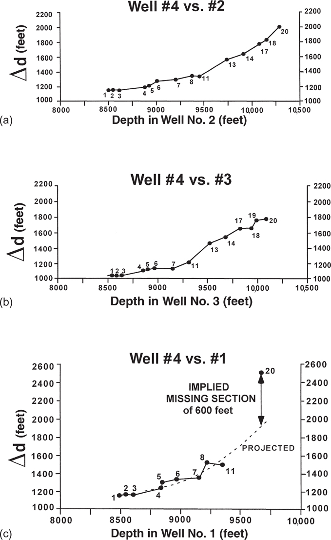
Figure 13-16 MBPA using Well No. 4 in Figure 13-15 as a reference well. (a) Growth plot using Well No. 2 for comparison. Growth increases monotonically between the 1 and 20 Horizons. (b) Growth plot using Well No. 3. Growth increases monotonically between the 1 and 20 Horizons. A comparison to Figure 13-5 shows no significant apparent missing section in either Well No. 2 or 3. (c) Growth plot for Well No. 1 located near the crest of the diapir. The plot suggests that about 600 ft of missing section exists at the level of the 20 Horizon. As 600 ft of section is not missing in Wells No. 2 and 3, or in other surrounding wells, the missing section in Well No. 1 is likely to result from a data miscorrelation, rather than a fault. (From Bischke et al. 1999. Published by permission of the Gulf Coast Association of Geological Societies.)
Figure 13-16c is a Δd/d plot for Wells No. 1 and 4, using the original correlations. Well log correlations are difficult below the 11 Horizon in Well No. 1. Notice where the correlation for the 20 Horizon appears in the Δd/d plot. The plot is subject to one of three possible interpretations:
The growth increases dramatically between the 11 and 20 Horizons around Well No. 1;
Based on the discontinuity in the plot, a normal fault or unconformity, with a missing section of about 600 ft, is present in Well No. 1 between the 11 and 20 Horizons; or
The 20 Horizon correlation in Well No. 1 is about 600 ft too high for a possible position of the 20 Horizon. We obtain the value of about 600 ft by projecting the growth curve, defined by the 1 to 11 data points, to beneath the 20 Horizon data point, and then determining the difference in depths.
Using the data obtained from the Multiple Bischke Plots and knowledge of the local geology, two of these interpretations can be eliminated and we can resolve the problem. We first consider the increased growth interpretation. Although dramatic increases in growth are possible, this increased growth is not observed in the nearby Wells No. 2 and 3 or in other nearby wells, thus making the high growth interpretation very unlikely.
The interpretation based on a 600-ft fault or unconformity can be rejected for the following reasons. A 600-ft unconformity should be observable on the down-dip portions of seismic profiles where bed dips are gentle or in growth plots constructed from other nearby, on-structure wells. Furthermore, Wells No. 1, 2, and 3 are drilled from the same platform, and Wells No. 2 and 3 are deviated more to the south than Well No. 1. If a large 600-ft fault cuts Well No. 1, then it could also cut Wells No. 2 and 3, or other nearby wells. Plots of the data shown in Figure 13-16a and b do not contain a large 600-ft discontinuity, nor do plots with other nearby wells. This means that the Δd/d plots do not indicate a large fault or unconformity below the 11 Horizon, making interpretation No. 2 also highly unlikely. Also, the seismic data over the structure is of reasonable quality. No large faults or unconformities are recognized on the seismic data near Well No. 1.
Reexamination of the well logs suggests that the correlation of the 20 Horizon, near the bottom of Well No. 1, is probably an incorrect correlation and that interpretation No. 3 is the likely solution. Additional correlation work indicates that the miscorrelated horizon, which is about 550 ft below the 11 Horizon in Well No. 1, is not the 20 Horizon, but rather it is most likely the 14 Horizon. This change in correlation results in a completely new interpretation from the 14 Horizon through the 20 Horizon. The changes affect the fault interpretation, structure maps, reservoir maps, and the upside prospect potential. The method results in a reasonable solution to a difficult problem in an area where well log correlation and 3D seismic data alone could not resolve the problem.
The Use of a Stacked Multiple Bischke Plot
This example, from the northern Gulf of Mexico, involves a salt-related structure. During the growth of salt diapirs, stratigraphic units onlap the flanks of the structures, creating large unconformities. Numerous faults associated with the growth sedimentation and developing structure may also be present, causing problems for a geoscientist who has to distinguish between missing section that results from faults and missing section that results from unconformities. Complicating the problem is the fact that the missing section caused by unconformities can exceed the missing section caused by growth faulting. Although this problem relates to salt, the general principles outlined in this section apply to locating unconformities in any tectonic setting.
Figure 13-17a shows well locations on the flank of a salt dome and the measured bed dips in the wells at a stratum called the Rob L Horizon. Figure 13-17b shows a Multiple Bischke Plot using the structurally higher Well No. 6 as a reference well. All the data from the off-structure wells can be plotted on the same diagram because each well is being compared to Well No. 6. This display, which emphasizes growth between the wells, is called a stacked plot (Chatellier and Porras 2001). Referenced along the x-axis are the Horizons B through Q in each well. Using the Multiple Bischke Plot, we can interpret the data. The structure experienced two growth phases, between the B and M Horizons and between the O and Q Horizons. The interval from the M to O Horizons exhibits little growth. Negative discontinuities are present in the plots of Wells No. 1 and 3. The discontinuities represent missing section, either due to a fault in the structurally lower well (compare to Fig. 13-5a) or due to downlap (compare to Fig. 13-6b). As downlap is rare on the flanks of salt diapirs, it is more likely that these discontinuities result from faulting in the structurally lower Wells No. 1 and 3. Correlation to other off-structure wells confirms that the missing sections in Wells No. 1 and 3 on the MBP are due to Fault J, which is noted on Figure 13-17b.
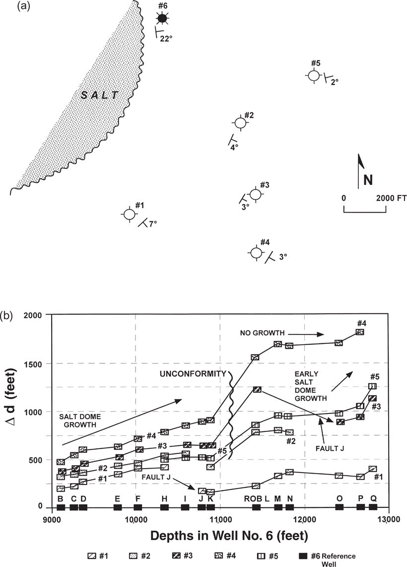
Figure 13-17 (a) Map showing strike and dip on the Rob L horizon at locations on the flank of a salt diapir in the northern Gulf of Mexico, USA. High bed dips on the flanks of salt structures cause stratigraphic thinning and deterioration of the seismic data. In this environment, geoscientists have difficulties attributing missing section to faults or to large unconformities. (b) The Multiple Bischke Plot for the structurally higher reference Well No. 6 versus the five off-structure comparison wells. The missing section above the Rob L sand in every well is interpreted to be due to a large unconformity. Fault J produces about 250 and 340 ft of missing section in Wells No. 1 and 3 respectively, based on the plot. (Published by permission of R. Bischke.)
On the flanks of salt diapirs, the amount of missing section typically increases up-dip as the horizontal distance between the on-structure and off-structure wells increases (Chapter 4, Fig. 4-44a). The Δd/d plots detect the amount of missing section caused by unconformities, as measured relative to the two wells used for a given plot. If both wells penetrate the same unconformity, then the amount of missing section determined from the plot will be the difference in the amounts of sections missing in the wells.
A positive discontinuity exists in every well plot in Figure 13-17b. Furthermore, this missing section occurs above the Rob L Horizon in every well plot. Thus, we attribute this missing section above the Rob L to represent an unconformity. The results of the MBPA guided additional correlation work and the interpretation when working with other structurally higher wells that flank the diapir.
Therefore, the MBPA, using six wells on this structure, provides quantitative graphical evidence for the following interpretation. The MBPA method (1) locates and defines the size (relative to certain wells) of the unconformity above the Rob L horizon, (2) defines the growth history of the structure, (3) provides initial evidence for Fault J, (4) aids in distinguishing faults from unconformities, and (5) helps keep the interpretation focused.
Vertical Separation Versus Depth Method
In Chapters 7 and 8, we discuss missing or repeated section resulting from normal or reverse faults as being equal to the fault component vertical separation (VS). The vertical separation can also be analyzed through the use of Multiple Bischke Plots. In the case of analyzing the vertical separation, the plots are now set up as VS/d rather than the normal Δd/d.
A plot of vertical separation versus depth can be used to analyze growth structures. In previous sections, we showed that information about tectonostratigraphic history is available by comparing two wells (Bischke 1994b). Outcrop, well log, depth-corrected seismic data, or well-constrained cross sections, provide the data required to construct the profiles. Now we apply vertical separation (VS) versus depth (d) plots to a variety of structural uses. The vertical separation data can be derived directly from seismic data or from missing or repeated section data obtained from correlation of well logs. These VS/d plots of data can be used to document fault growth and timing, and to determine structural style. If the structural style in an area is complex or ambiguous, then the profiles can help to determine the correct structural style. A number of generic and real examples presented in this section illustrate how to apply the method.
If geoscientists can correlate across a fault surface, then they can construct maps of faulted horizons. These maps contain information on the tectonostratigraphic history (Yeats and Beall 1991). The VS/d method records the vertical distance that correlative beds displace across fault surfaces. Geoscientists define this vertical distance between offset beds, on opposite sides of a fault, as vertical separation (Chapter 7). As opposed to other fault displacement components, geoscientists can always determine the vertical separation component of fault displacement. For example, slip measurements require a 3D understanding of fault displacements. One-dimensional well logs and two-dimensional seismic profiles do not contain 3D information, and they cannot independently provide slip measurements (Chapter 7). Fault throw may be obtainable only after the construction of 3D maps, or from seismic sections that are perpendicular to the strike of the fault surfaces (Chapter 8).
The VS/d plots measure the vertical component of fault displacement. We typically think of vertical separation for normal and reverse faults. However, strike-slip faults also commonly exhibit vertical displacements (Harding 1973; Wright 1991; Shaw et al. 1994), particularly at restraining and releasing bends (Crowell 1974a and b) (Chapter 12). Also, because paleotopographic surfaces are not planar and strike-slip faults exhibit vertical slip components, the method can apply to growth sedimentation associated with strike-slip faults (Shaw et al. 1994).
Where subsurface data are sparse, the construction of subsurface maps and cross sections typically involves the introduction of assumptions and interpretation. Fault slip components are rarely obtainable in outcrop data, making fault slip determinations questionable even where faults are subject to direct observation. However, VS is always obtainable directly from missing or repeated section in well logs or from a single seismic profile (Chapter 7). Thus, we present a method for studying fault displacements based on VS.
Method
Information on fault history and structural style is obtainable by plotting VS against the depth of the faulted horizons at the footwall cutoff (Fig. 13-18). Every displaced horizon has a value of VS (VS1, VS2, VS3, . . . VSn). For a VS/d plot, the VS is measured from the footwall horizon to the hanging wall horizon. For a normal fault, the footwall horizon is projected across the fault (Fig. 13-18). The measurement of VS in these cases is downward (increasing depth), and the amount of VS is taken to be a positive value for purposes of the VS/d plot (Fig. 13-18). For a reverse fault, the measurement of VS is upward (decreasing depth), and the amount of VS is taken to be a negative value (Fig. 13-19).
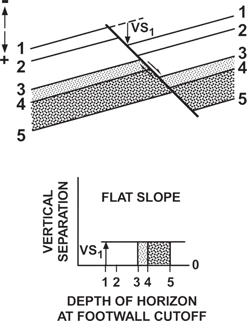
Figure 13-18 A generic example of a post-depositional normal fault and its VS/d plot. A post-depositional normal fault plots in the positive quadrant and has a flat slope. (Published by permission of R. Bischke.)
If the fault exhibits growth, then sediments deposited coeval with fault motion will change thickness across the fault surface, and the values of VS will change with depth. The slope of the VS/d plots can be used to define fault growth, with higher slopes indicating higher growth rates. A zero slope indicates a post-depositional (nongrowth) fault (Figs. 13-18 and 13-19). So, the method readily defines the timing of fault movements.

Figure 13-19 A generic example of a post-depositional reverse fault and its VS/d plot. A post-depositional reverse fault plots in the negative quadrant and has a flat slope. (Published by permission of R. Bischke.)
The plots of VS versus depth document vertical displacements. If age data are available, then it is possible to determine the displacement history within a time framework. However, the plots cannot independently detect large rotational motions (see Chapter 12). Where applicable with seismic data, use the workstation to convert the seismic data to depth before constructing the plots. Typically, interval velocities are adequate, although better velocity versus depth functions improve the results.
Generic and Real Examples of Analysis of VS/d Plots
Vertical separation data taken along fault surfaces provides information on fault displacement history and structural style. Thus, in this section we concentrate on fault surfaces. The data required are VS measurements and the depth to the footwall cutoff of each correlated horizon. We present a number of generic and real examples of several common, and some less known, structural styles. There are two basic types of faults, growth (expansion) faults and post-depositional (nongrowth) faults (Thorsen 1963). The plots of VS versus depth document growth faulting or post-depositional faulting. Our discussion starts with simple examples, followed by more complex ones.
Post-Depositional (Nongrowth) Faults.
Correlative stratigraphic intervals on opposite sides of post-depositional faults do not exhibit significant thickness changes across fault surfaces. As VS does not change with increasing depth, post-depositional faults exhibit zero (flat) slopes on VS/d plots (Figs. 13-18 and 13-19). As a matter of convention, we define normal faults to contain positive displacements. Thus, post-depositional normal faults plot above zero VS and in the positive quadrant (Fig. 13-18). The reason for distinguishing between positive and negative quadrants will become clear in the Complex Growth Structures section.
In contrast to the normal fault, the sign of VS along a post-depositional reverse fault is negative, and thus reverse faults plot in the negative quadrant (Fig. 13-19). So, on VS/d plots, reverse and normal faults plot in different quadrants. Post-depositional reverse faults exhibit flat slopes on VS/d plots, as do the post-depositional normal faults (compare Figs. 13-18 and 13-19).
Growth Normal Faults.
Sedimentary units change thickness across faults when the sedimentation is concurrent with faults that have dip-slip components of displacement. Growth associated with faulting is common in areas that have rapid sedimentation rates (Suppe et al. 1992; Shaw et al. 1994), and thus normal, reverse, and strike-slip faults may exhibit growth. One can distinguish growth faults from post-depositional faults in that the growth faults have nonzero slopes on the VS/d plots. The VS/d method has a high resolution and can detect growth where growth is not obvious in surface or subsurface data. The expansion faults common to deltas exhibit positive slopes on the VS versus depth plots, and the data are in the positive quadrant (Fig. 13-20).

Figure 13-20 A generic example of a growth normal fault and its VS/d plot. A growth normal fault plots in the positive quadrant and has a positive slope. (Published by permission of R. Bischke.)
Figure 13-21 is a VS/d plot for a growth fault in the northern Gulf of Mexico. Growth Faults tend to seal through an interval of rapid growth, and any faults with large displacement tend to seal. The larger the fault, the greater the probability that the fault will seal. Large displacements on a fault can create a clay smear or barrier in the fault zone or can juxtapose permeable rocks against shale (Brenneke 1995). In the United States, strata are typically dated by index fossil taxa, such as Cibicides optima (abbreviated CIB.OP.). A review of Figure 13-21 shows that the earliest growth on the fault occurred just prior to CIB.OP.-10 time, with the older faulted interval being pre-growth strata. The fault grew rapidly from CIB.OP.-10 time to about Bigenerina (3)-1 [BIG.(3)-1] time, and then became inactive. Just before Textularia (W)-2 [TEX.(W)-2] time, the fault became active again and continued growing, at a decreasing rate, until Bigenerina (A)-1 [BIG.(A)-1] time. As the fault exhibits 400 ft to 900 ft of vertical separation and was growing rapidly during CIB.OP.-10 time to BIG.(3)-1 time, the fault has a high probability of sealing below the 11,000-ft level.
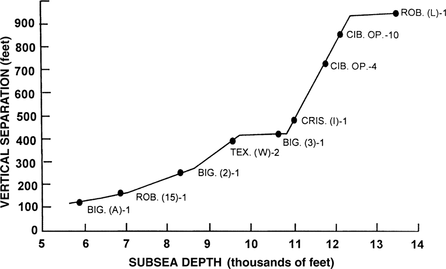
Figure 13-21 VS/d plot illustrating fault timing on a normal fault from the northern Gulf of Mexico, offshore USA. Rapid growth on the fault, between 11,000 ft and 12,400 ft, enhances its trapping capabilities within that depth range. (Published by permission of R. Bischke.)
Growth Reverse Fault.
Most geoscientists know that growth faulting is common to extensional environments. Less well known is the case where deposition is concurrent with folding and/or reverse faulting, and compressional growth structures form (Suppe et al. 1992; Tearpock et al. 1994; Chapter 10 of this book). If, during compressional folding, the sediments flood across and over the rising structure, then a compressional growth structure forms (Fig. 13-22). Plots of VS versus depth for growth reverse faults are distinguished from those of growth normal faults in that they exhibit negative slopes and plot in the negative quadrant (Fig. 13-22).
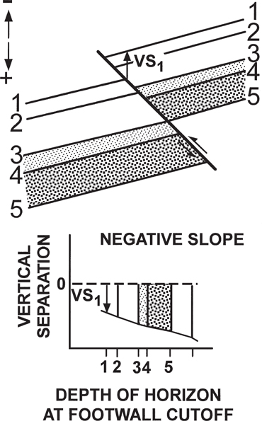
Figure 13-22 A generic example of a growth reverse fault and its VS/d plot. A growth reverse fault plots in the negative quadrant, with a negative slope. (Published by permission of R. Bischke.)
Complex Growth Structures.
Complex growth structures exist where more than one fault, or slip surface, is present, or where there was more than one period of deformation. Complex structures occur in all tectonic environments. The hybrid inversion structures that occur in Brunei (James 1984), the North Sea (Mitra 1993), Venezuela (Link et al. 1996), and elsewhere are readily recognizable on the VS/d plots. Inversion structures originate as normal fault structures that are later subject to reverse fault displacements. Growth across the faults may be noticeable during both the extensional and compressional phases. On growth plots, the VS data initially plot in the negative and then in the positive quadrant (Fig. 13-23). As these structures plot in different quadrants and have positive slopes, inversion structures are distinct and easily recognized from other fault styles.

Figure 13-23 A generic example of an extensional, growth inversion fault and its VS/d plot. An extensional growth inversion fault plots in both the positive and negative quadrants, with a positive slope. (Published by permission of R. Bischke.)
Inversion structural styles have been easily confused with strike-slip fault structural styles. In Chapter 12, we discuss methods and procedures for documenting horizontal displacements, which are critical in determining strike-slip faulting. Plots of VS versus depth aid in recognizing inversion structures. In the hanging wall portions of inversion structures, the shallow stratigraphy is thin relative to its correlative footwall units, whereas the deeper stratigraphy is thick relative to its correlative footwall units (Fig. 13-24 and Mitra 1993). Before the recognition of inversion structures, and on older seismic data that poorly imaged the listric normal fault, geoscientists commonly interpreted well log and seismic data incorrectly. We use a depiction of an inversion structure in Venezuela as an example. First, at the shallow structural level of the stratigraphic unit, geoscientists recognized that the thin, shallow-water environment, footwall stratigraphy correlated to the thicker, deep-water environment strata in the hanging wall block (Fig. 13-24b). Second, the thickness of the sediments and the environmental conditions reverse at the shallower structural level, with the footwall section being thicker relative to the hanging wall section. The deeper, and once downthrown, units were subsequently thrust back up, along the pre-existing normal faults. This reverse motion thrusts the deeper water units to a structurally higher level than the correlative thin shallow water units (Fig. 13-24b). Before the recognition of inverse structures, these complex and confusing relationships were interpreted to result from large strike-slip displacements. Only strike-slip displacements were considered capable of creating this confusing geometric style. Thus, inversion structures may be misidentified as “flower” structures. To help distinguish inversion structures from flower structures, examine the correlation markers on VS/d plots. If the markers plot in both the negative and positive quadrants and have positive slopes, then the structure is most likely an inversion structure.
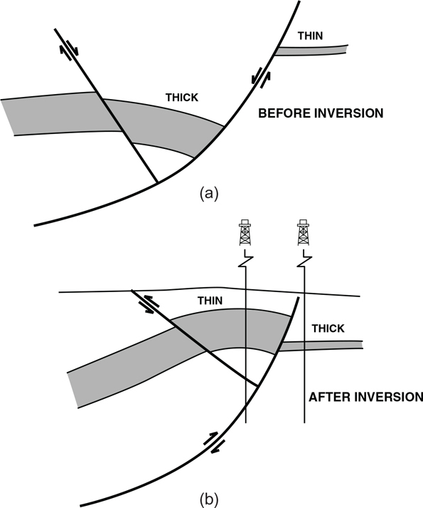
Figure 13-24 Schematic example of inversion. As the displacements reverse on an inversion structure, the thick, originally downthrown section is subsequently thrust back over a thin correlative section located in the footwall. Geoscientists often interpreted these confusing stratigraphic and structural relationships to result from strike-slip faulting. (Published by permission of R. Bischke.)
We can distinguish between an inversion structure and another structural style. Compressional inversion structures are present where the displacements on reverse faults invert and become normal. The positive and negative data points, combined with negative slopes, indicate inversion on a VS/d plot (Fig. 13-25).

Figure 13-25 A generic example of a compressional, growth inversion fault and its VS/d plot. On a compressional, growth inversion structure, the thin upthrown section is later downthrown, juxtaposing thin sections in the hanging wall against thicker sedimentary sections in the footwall. A compressional inversion fault plots in both the positive and negative quadrants and has a negative slope. (Published by permission of R. Bischke.)
Downward-Dying Growth Faults.
Another important but problematic structure is the downward-dying growth fault, which commonly forms in the extensional environment (Bischke and Suppe 1990b; Tearpock and Bischke 1991). Some geoscientists err in being unaware that a normal fault may die downward. An extension of a fault with depth is unreasonable if supporting data does not exist. However, this fault style can be recognized because it plots on a VS/d diagram in the positive quadrant and exhibits positive slopes at shallow depths and negative slopes at greater depths (Fig. 13-26).

Figure 13-26 A generic example of a downward-dying, growth normal fault and its VS/d plot. The displacements on downward-dying faults decrease with increasing depths. A downward-dying growth fault plots in the positive quadrant. It has a positive slope at shallower depths and a negative slope at greater depths. (Published by permission of R. Bischke.)
Some faults in deltaic areas may decrease in displacement in all directions away from a central point. If the vertical separations on these faults surfaces are contoured into a map of fault displacements, then these faults exhibit a more or less elliptical displacement pattern (Barnett et al. 1987; Bergen and Shaw 2010). The maximum displacements occur at the center of the ellipse and the fault dies out in every direction, upward, downward, and laterally. In Chapter 11, we present a model to explain these unusual relationships in a syntectonic depositional environment.
Figure 13-27 shows a map of a downward-dying growth fault, with accompanying seismic section, and a VS/d plot (Rabbit Island, coastal Gulf of Mexico, USA). The Rabbit Island fault exhibits 450 ft of missing section in a well at the 5500-ft level and about 70 ft of missing section in a well at about the 11,000-ft level. The structural question is, what happens to the fault below 11,000 ft? In order to determine the downward extent of the fault, based only on well control, there must be wells that go deeper than 11,000 ft in the area where the fault could reach this depth. With seismic data, one must approach the interpretation with caution. At times, interpreters do not pay attention to the displacements when picking faults, but rather they concentrate on interpreting the fault location on the seismic sections. If an interpreter does not realize that he or she is dealing with a downward-dying fault, an interpretation can be generated of a throughgoing fault extending to depth. This apparent throughgoing fault may set up prospects or perhaps divide producing reservoirs. If the fault in our example is absent beneath the 11,000-ft level, then no fault exists to trap hydrocarbons beneath that level. Or, if a reservoir exists just beneath 11,000 ft, then the partitioning of the reservoir is incorrect. In either case the interpretation is wrong and can have serious implications to any exploration or development activities. Geoscientists can construct VS/d plots to predict fault displacement and to evaluate whether they are dealing with a downward-dying fault, and to determine at which level the downward-dying fault loses its displacement (Tearpock et al. 1994). The Rabbit Island fault apparently dies out near the 11,000-ft level, as shown on the seismic line in Figure 13-27c, and it cannot trap hydrocarbons beneath that depth.
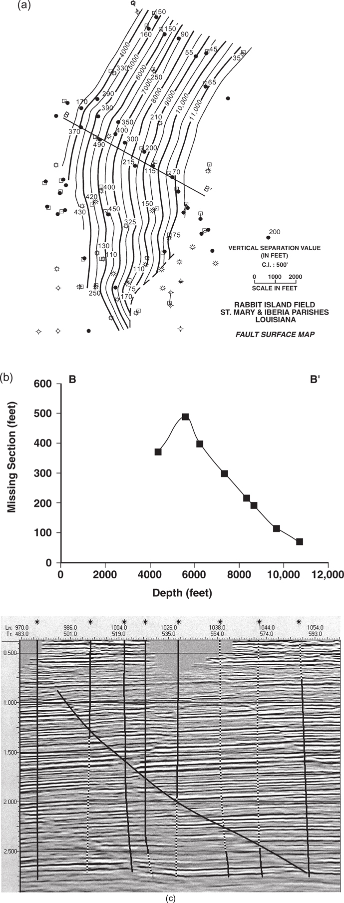
Figure 13-27 (a) Map, (b) VS/d plot, and (c) seismic line showing a downward-dying growth fault in Rabbit Island Field, coastal Gulf of Mexico, USA. Vertical separation decreases with increasing depth. The trapping capabilities along the fault surface diminish at about the 11,000-ft level. Figures 13-27a and b interpreted by D. Tearpock. (Maps and seismic line published by permission of Texaco, Inc.; VS/d plot published by permission of R. Bischke.)
Downward-dying growth faults are common in many areas, and seismic displays of them from the northern Gulf of Mexico and Brunei are in Chapter 11. In other areas, some faults may extend to depth, whereas other faults die downward. When dealing with potential hydrocarbon traps on downward-dying faults, care must be exercised to be sure that the potentially trapping fault will offset the objective horizon (Tearpock et al. 1994). The VS/d method or MBPA can aid in the recognition and documentation of the trapping capability of downward-dying growth faults.
Conclusions
Reliable correlation data are obtainable in many areas, but the data may deteriorate in key areas. The Δd/d, MBPA, or VS/d methods, when integrated with geological and geophysical data, can resolve difficult structural and stratigraphic problems where 3D seismic and well log correlation data are ambiguous (Sanchez et al. 1997). The methods are easy to use, require little additional effort, and can eliminate the guesswork that could lead to incorrect structural interpretations and maps that could result in dry holes. Where correlation problems result from complicated structural features, the Multiple Bischke Plot Analysis can resolve these problems during the initial stages of a project, prior to constructing subsurface maps and generating prospects. This can help eliminate the need to remap the structure and/or reinterpret the seismic and well log data at a later stage in a project.
Additionally, as the methods are easy to use and rapid to apply, they serve as excellent checks on any interpretation involving structures or correlations. Often, after finishing a project, interpreters assume that their interpretations and maps are correct and do not subject their interpretations to consistency checks (Tearpock et al. 1994). This can result in interpretations that are inconsistent with the interpreter’s own correlation data, maps, or cross sections. Growth techniques are an excellent consistency check and introduce a relative age factor into interpretations. Managers may find these techniques useful during prospect reviews and when analyzing prospects and the petroleum system.
The Δd/d and MBPA methods have a resolution of about one part in a thousand when using well log data, so the methods can often identify disconformities, subtle systems tract boundaries, or small growth faults (Bischke 1994b). The techniques can distinguish faults from unconformities where bed dips are high and where the seismic data is incoherent. If a well log correlation is the probable cause of the problem, then the method can direct geoscientists to the correct correlation, thus eliminating guesswork. Analysis of growth history often leads to viable structural solutions to complex problems.
Syntectonic sedimentation can occur in any tectonostratigraphic regime, not solely in the extensional, normal fault regime. In areas where the sedimentation rates keep pace with the tectonic uplift rates, structures formed by compressional and strike-slip faults can exhibit growth (Suppe et al. 1992; Shaw et al. 1994). These growth environments allow for the determination of fault timing that influences migration and petroleum system studies. Lastly, in areas where structure is complex or ambiguous, growth plots provide the results to determine structural style and resolve interpretation problems. Any interpretation of a stratigraphic sequence or structure must be consistent with the correlations.