Chapter 8. Structure Maps*
* For all figures in this chapter (in the printed book only), see the preface for information about registering your copy on the InformIT site for access to the electronic versions in color.
Introduction
The subsurface structure map is one of the primary vehicles used by geoscientists to find and produce hydrocarbons from the initial stage of exploration through the complete development of a field. Each subsurface structure map is a geological or geophysical interpretation based on limited data, technical proficiency, creative imagination, 3D visualization, and experience. We consider the construction of a structure map to be an interpretive and creative process. No two geoscientists will construct a map exactly the same, even with the same data, because each uses the factors just mentioned in addition to educational background and field experience to develop his or her interpretation. However, the interpretation must incorporate sound geological principles, correct and accurate mapping techniques, and be valid in three dimensions.
The importance and reliability of subsurface structure mapping increase with advancing stages of field development and depletion. Many management decisions are based on the interpretations presented on subsurface structure maps. These decisions involve investment capital to purchase leases, permit and drill wells, and to work over or recomplete wells, to name a few examples. A geoscientist must employ the best and most accurate methods to find and develop hydrocarbons at the lowest cost per net equivalent barrel.
Since faulted structures play such a significant role in the trapping of hydrocarbons, we devote a considerable portion of this chapter to the correct and accurate subsurface mapping techniques required to integrate fault surface map interpretations into the structural interpretation to construct completed structure maps. A reasonable structural interpretation, in most faulted areas, begins with an accurate fault picture developed from the interpretation of faults and the construction of fault surface maps using fault data from well logs and seismic sections (Chapter 7), followed by the integration of these fault surface maps into the structural interpretation.
Many petroleum provinces involve multiple faults that result in extremely complicated structural relationships. The attempted reconstruction of a complex structure with isolated fault data from well logs or seismic sections can result in erroneous geological interpretations. Too often, subsurface interpretations and the accompanying structure maps are prepared without giving much consideration to the 3D geometric validity of the interpretation. The most accurate and sound structural interpretation in a faulted area requires (1) the interpretation and construction of fault surface maps for all important structure-forming and trapping faults, (2) the integration of the fault surface maps with the structural horizon maps, and (3) mapping of multiple horizons at various depths (shallow, intermediate, and deep) to justify and support the integrity of any structural interpretation (Tearpock and Harris 1987).
The exploration for and exploitation of hydrocarbons is interpretive and creative work. Most of the time, a geoscientist is dealing with geological structures that are not visible on the surface. The formidable challenge of interpreting these unseen structures can be accomplished only with a clear understanding of basic geological principles, familiarity with the geometry of structural and fault surface relationships, analysis of all available data, use of all technical capabilities, application of technical knowledge and skills, and imagination.
In this chapter, we concentrate on the technical knowledge and skills necessary to develop a geologically reasonable structural interpretation. Technical knowledge and skills fall into two categories: (1) a good understanding of the tectonic setting being worked, and (2) understanding and application of correct interpretation and mapping techniques. The primary focus of this chapter is on the broad range of important structural mapping techniques; however, since the application of many techniques depends on the tectonic style (type of structure and trap), we discuss and illustrate techniques as they apply to different tectonic settings and review a number of real-world examples.
Subsurface structure maps usually are constructed for specific stratigraphic horizons to show, in plan view, the geometric shapes of these horizons. These maps are constructed using correlation data from well logs, interpretations of seismic sections, and in some cases, outcrop data. Remember that accurate correlations are paramount for reliable subsurface interpretation and mapping. Subsurface structure maps are no more reliable than the correlations used in their construction. Incorrect correlations will find their way, at some point, into the final interpretation. They may be incorporated into the fault, structure, isochore, or isopach maps and result in serious mapping problems. Therefore, it is essential that utmost care be taken in correlating logs and interpreting seismic sections.
Not every horizon within a stratigraphic sequence is suitable for structure mapping. A horizon that is not correlatable over a large area or one that is limited in areal extent may not be suitable. Maps on stratigraphic horizons of limited extent, if important, can be prepared after the overall structural interpretation has been developed from fieldwide or regional correlations and structure maps.
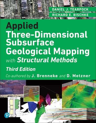
A structure map is a form of contour map. As discussed in Chapter 4, marine shales exhibit distinctive characteristics over large areas. Therefore, they serve as good correlatable horizons for fieldwide or regional structure mapping. A structure contour map presents a 2D interpretation of the 3D shape of a specific stratigraphic horizon. Each contour connects points of equal elevation above or below sea level for a given stratigraphic horizon. A good structural interpretation requires 3D thinking, as illustrated in the simplified block diagram in Figure 8-1.
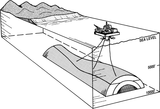
Figure 8-1 A 3D view of an anticlinal structure 7000 ft below sea level.
Broadly interrelated assemblages of geological structures constitute the fundamental structural styles of petroleum provinces. These assemblages generally are repeated in regions of similar deformation, and the associated types of hydrocarbon traps can be anticipated (Harding and Lowell 1979). There are a number of petroleum-related tectonic habitats around the world; each results, to varying degrees, in different kinds of hydrocarbon traps that may require modified or different mapping techniques. In the first part of this chapter, we discuss numerous subsurface structure mapping techniques. These techniques are then reviewed as they apply to the following tectonic habitats and their associated hydrocarbon traps.
Extensional terranes, including normal faulting and detached listric growth fault systems.
Compressional terranes, including reverse faulting and fold and thrust belts.
Diapiric salt terranes.
Strike-slip fault terranes.
Guidelines to Contouring
Review the five basic rules of contouring presented in Chapter 2. In addition to these basic rules, the following guidelines to contouring make a map easier to construct, read, and understand; they also help to ensure the technical accuracy and correctness of the completed map. Some guidelines covered in Chapter 2 are repeated here; many have been expanded, and additional guidelines are presented.
All contour maps must have a chosen reference to which the contour values are compared. A structure contour map usually uses sea level as the chosen reference. Therefore, the elevations on the map can be referenced above or below mean sea level. A negative sign in front of a depth value indicates that the elevation is below sea level.
The contour interval on a map should be constant. The use of a constant contour interval makes a map easier to read and visualize in 3D because the distance between successive contour lines has a direct relationship to the steepness of slope. Steep dips are represented by closely spaced contours, gentler dips by contours with a wider spacing. Figure 8-2 illustrates the confusion and difficulty involved in trying to visualize a contoured surface in 3D where the contour interval is not constant over the mapped area. From fault block to fault block, the contour interval changes from 100-ft to 50-ft contours with no consistency. Notice upthrown to Fault A that the contour interval is 50 ft, and downthrown it is 100 ft, yet the contour spacing is about the same. This indicates that the area downthrown to Fault A has a much steeper dip than the area upthrown. However, when we look at this area of the map, the contour spacing gives the illusion that the dip rate in both fault blocks is about the same. The contour interval changes even within the fault block northeast of Fault A.

Figure 8-2 This structure map has an inconsistent contour interval randomly changing from a 50-ft to 100-ft contour interval from fault block to fault block. Such inconsistency in the contour interval makes a map difficult to visualize in three dimensions. Observe the change in contour interval upthrown and downthrown to Fault A, and even in the fault block upthrown to Fault A. (From Tearpock and Harris 1987. Published by permission of Tenneco Oil Company.)
The choice of a contour interval is an important decision. Factors to be considered include the density of data, the practical limits of data accuracy, the steepness of dip, the scale, and the purpose of the map.
Contour spacing depends on the dip of the structure being mapped. For any given structure, the spacing of contours will vary at different locations unless the equal spacing method of contouring is used. Several graphs are designed for convenient use to compute contour spacing when the dip is known; likewise, the dip on a completed map can be determined by measuring the contour spacing [see Eq. (2-2)]. Figure 8-3 is a graph that relates the dip of beds to the horizontal distance between 100-ft contours. It can be used for determining dip or contour spacing for fault maps as well as structure maps.
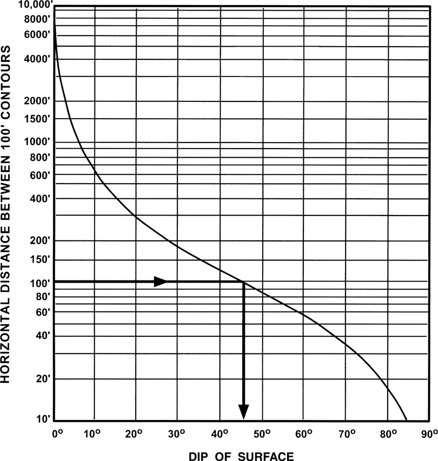
Figure 8-3 Graph of dip versus horizontal distance (in feet) between 100-ft contours. This graph is derived from Equation 2-2, bed dip = arctan (contour interval/contour spacing), also described as bed dip = arctan (rise/run).
All maps should include an X-Y graphic scale (Fig. 8-4). A graphic scale gives the viewer an idea of the areal extent of the map and the magnitude of the features shown. Maps are commonly reduced or enlarged for various reasons; without a graphic scale, the values shown on the map become meaningless. This is especially true for maps that might be displayed as slides during meetings. The ability of computers to cut, paste, stretch, and squeeze maps requires the use of X-Y scales.
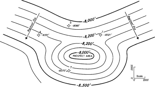
Figure 8-4 An example of a localized structural high indicated by a change in regional dip.
Every fifth contour is an index contour. It should be bolder or thicker than the other contours and labeled with its value (Fig. 8-4).
Hachured lines should be used to indicate a closed depression (Fig. 8-5).
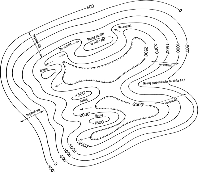
Figure 8-5 A diagrammatic structure contour map of a basin illustrating several important contouring guidelines. (From Bishop 1960. Published by permission of author.)
Contouring should be started in areas with the maximum number of control points (Chapter 2, Fig. 2-8). The area or areas of maximum control commonly occur around structural highs or lows.
Construct contours in groups of several lines rather than one single contour at a time (Fig. 2-8). This method provides better visualization of the surface being contoured and results in more consistent contouring.
Initially, choose the simplest contour solution that honors the control and provides a realistic interpretation. The simplest solution may be the best (Occam’s razor), and it is usually easy to test. If problems arise with this solution, a more complex interpretation can be prepared.
Use a smooth rather than undulating style of contouring unless the data indicate otherwise. Some geoscientists argue that a smoothly contoured structure is not likely to occur in nature (Chapter 2, Fig. 2-9). This may be true; however, it is better to keep the structure simple with smooth contours until the data indicate otherwise. It is possible to present a significant misinterpretation by placing unjustified wiggles in contours (Silver 1982).
Initially, a hand-contoured map should be contoured in pencil with lines lightly drawn so that they can be erased as the map requires revision.
Establish regional dip whenever possible. Regional dip is the general direction of dip for any given area. Regional dip may not be constant over a large area, but changes should be gradual. In areas of regional dip, contour lines have a certain degree of parallelism along regional strike. Any change in the dip rate may be an indication of local structures. In areas of minor or localized structures, contours extend away from regional dip. Such indications are important because in many petroleum provinces minor anomalous highs that break regional dip commonly are productive of hydrocarbons (Fig. 8-4).
If regional dip is interrupted by a localized structural high, reentrants occur on each side of the minor uplift (Fig. 8-4 or 8-5). If the axis of the localized uplift parallels regional strike, the magnitude of the reentrants may be small compared to reentrants adjacent to a high that is perpendicular to regional strike (Fig. 8-5).
Any flattening or reversal of normal dip is a possible clue to local structures. Therefore, changes of this kind are extremely important. Local uplifts may have their axes perpendicular or parallel to the regional strike. When the axis of a local fold is perpendicular to strike, contours flare outward in a down-dip direction and the distance between contour lines increases as the rate of dip decreases. A nosing or U-shaped projection results in the bottom of the U pointing basinward (Fig. 8-5). Nosings are flanked by reentrants, the axes of which may be perpendicular or oblique to the regional strike. The reentrants begin where the contours start to widen out and are less pronounced down-dip until eventually they disappear.
If the axis of a structurally high area is parallel to regional strike, reentrants are also parallel to strike. As the direction of regional dip reverses at the axis of the reentrants, a high area results down-dip, as shown in Figure 8-5 (Bishop 1960).
Contouring can be optimistic or pessimistic depending on your experience, corporate guidelines, and exploration philosophy. All contouring, however, must be governed by sound geological principles and the general tectonic style, and optimism must be kept within geologically reasonable limits. Pessimistic contouring can condemn potentially prospective areas to the point that no exploratory drilling is undertaken. A good mapping philosophy to follow is to map neither optimistically nor pessimistically, but instead use all of your technical expertise to map realistically. Structure maps used to determine reserves (Chapter 14) should generally be contoured conservatively.
In areas of either limited subsurface control or vertical faults, it is important to contour the limited data to reflect as simple a geological interpretation as possible, rather than just to connect points of equal elevation. Therefore, any radical change that occurs in the strike of the contours may suggest faulting even though no fault has been recognized by well control. Figure 8-6a depicts such a situation. In these cases, all available data need to be reviewed, including production and pressure data to help resolve the geological problem. In the example shown in Figure 8-6, notice a significant change in contour strike in the area marked as a possible fault, although no fault is recognized in the wells. An interpretation that fits all the geological and hydrocarbon data includes a vertical fault not intersected by the wells (Fig. 8-6b).
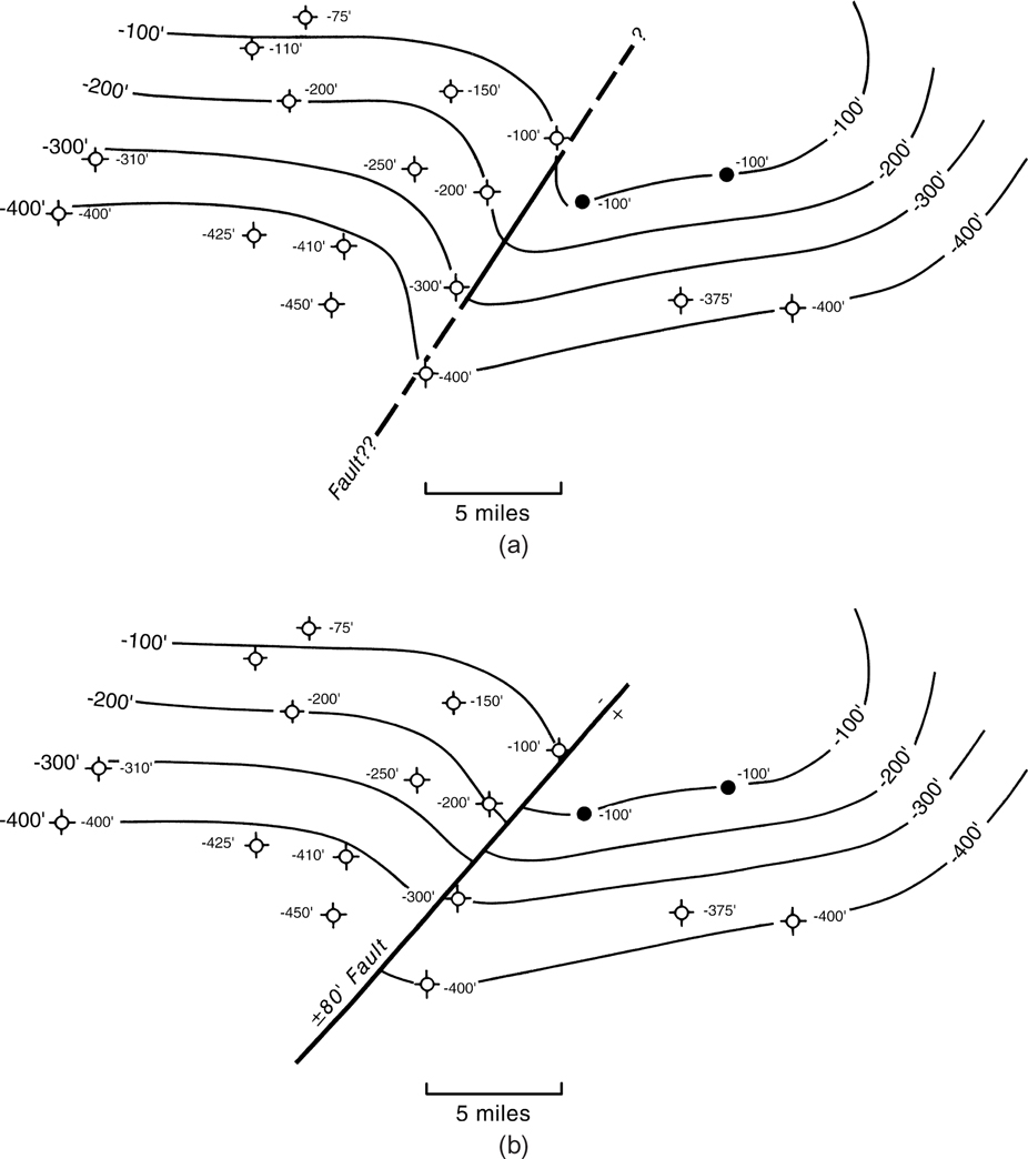
Figure 8-6 (a) An abrupt change in the strike direction of contours suggests the possibility of faulting. (b) Another interpretation of the data in Figure 8-6a that fits the geological and hydrocarbon data includes a vertical fault not intersected by the wells. (Modified after Bishop 1960. Published by permission of author.)
An abrupt increase in the rate of dip is a good indication of faulting. An increase in the rate of dip accompanied by an abrupt change in strike is very strong evidence of faulting (Bishop 1960). Increased dip might, alternatively, result from folding, but in most cases the increase is more abrupt where faulting is responsible.
A change or reversal in the direction of dip suggests the crossing of a fold axis (Fig. 8-5 or 8-7). Reversal of dip may occur over the crest of an anticline or the trough of a syncline. The amount of dip reversal is often a guide to whether the reversal is due to a regional change or local structure. An excessively steep dip may indicate the presence of a fault or steep fold, while a dip that flattens may be indicative of the crest of a fold or the bottom of a syncline.
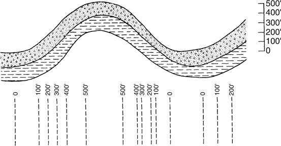
Figure 8-7 Structural highs and lows can sometimes be recognized by their effect on contour spacing. (From Bishop 1960. Published by permission of author.)
Structures may or may not have structural attitude compatibility (contour compatibility) across a fault. The compatibility of structural attitude on opposite sides of a fault depends primarily on the size and type of fault. For example, within many, if not most, structures, structural compatibility exists across normal and reverse nongrowth faults (Fig. 8-8a). In contrast, many large listric normal faults (such as growth faults) and thrust faults, with significant displacements, result in structures that are not compatible across the large fault (Fig. 8-8b). Large listric normal faults and large thrust faults create structures such as rollover anticlines, fault bend folds, and fault propagation folds. If the fault creates the structure, you should not expect contour compatibility across the fault, although there may be compatibility across smaller faults within the created structure. The method of structure contouring across a fault depends on whether there is a compatibility of structural attitude on both sides of the fault.
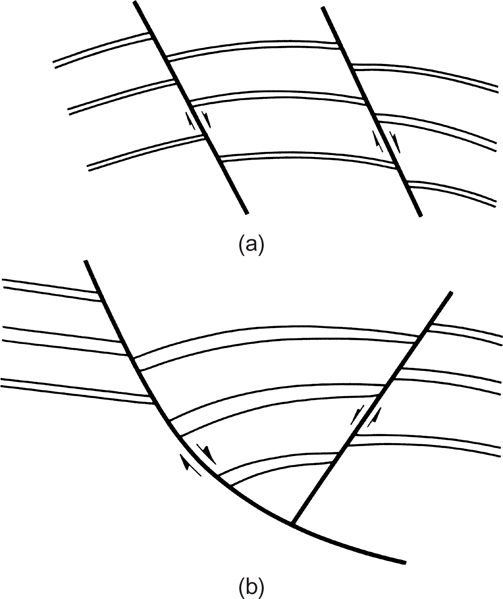
Figure 8-8 (a) Cross section shows structural compatibility across faults. (b) Cross section shows no structural compatibility across major growth fault, but structural compatibility across the smaller antithetic fault.
Structural highs, regardless of origin, usually tend to flatten across the axis with gentle dips across the top of the structure (Fig. 8-7). Exceptions do occur, such as the structure in the inner core of a fault propagation fold (Chapter 10). Contour line spacing widens across the crest of the structure compared to spacing on the flanks. Synclines, like anticlines, also tend to flatten across their axes. The widening of contours is often even more pronounced in a syncline. If the data indicate a continuously steep slope up to the crestal high with little if any flattening of dip, this may indicate that the surface is one that has been affected by erosion (the presence of an unconformity).
Closed structural lows are not common. If possible, avoid closing lows with contours unless the data require it. The presence of closed lows often suggests an eroded surface or the presence of faulting. If the closed low is elongated, faulting is likely, and the greater the size of the closed low, the greater the probability of faulting.
Contour license refers to the geologist’s right to contour a structure in a way that best fits the geological, geophysical, and engineering data, and that best represents the types of structures present in the tectonic setting. The interpretive method of contouring as defined by Bishop (1960) best corresponds to what we call contour license. The use of geological license requires a solid educational background and extensive experience. Contour license does not allow a geologist or geophysicist to ignore or misrepresent valid data.
Specific structural highs may be in the form of domes, anticlines, and noses. Domal structures are usually the result of local positive features, such as diapirs, that provide relative uplift. On the flanks of domes, the direction of dip is away from the central high and the dip rates are commonly constant along strike, at least within each major fault block around the structure. Therefore, the contour spacing is commonly uniform along strike. In the dip direction, the structurally highest areas on the flank typically have the steeper dips, with a gradual decrease in dip away from the uplift. Contour spacing is close high on the flank of the structure, but widens with distance down-dip.
Anticlinal structures generally appear as elongated domes. Their origin can be the result of compressional forces (e.g., fault-propagation folds associated with reverse faults), extensional forces (e.g., rollover anticlines associated with growth normal faults), or strike-slip forces. In general, the direction of dip is away from the crestal area in two opposing directions. Since anticlines are commonly asymmetric, with inclined axial surfaces, the dip rate and resulting contour spacing may vary around the anticline.
Structural noses that trend off local structures show dip away from the crest in three directions. Contour lines widen, indicating flatter dips in the area of a nose or an associated reentrant. Contours become closer together immediately down-dip of the local high until regional dip is attained again.
The best test of the 3D geometric validity of any structure contour map is its predictability. How well does the interpretation hold together with additional data from the drilling of new wells or the shooting of new seismic lines? If the interpretation and maps require major revision each time new data are obtained, there should be serious concern regarding the validity of the interpretation and accompanying maps. On the other hand, if only minor adjustments are required and hydrocarbon traps predicted by the mapping are successfully found, the interpretation may be considered reasonable. Remember, we always work with a limited amount of subsurface data to be interpreted. Each geoscientist must have imagination, an understanding of local structures, the ability to visualize in three dimensions, a sound geological education, field experience, and technical knowledge and skills to evaluate any number of possible (alternative) interpretations. Finally, a geoscientist must decide which interpretation, in his or her judgment, is the most reasonable. The 20 guidelines presented in this section should help you construct more accurate and reasonable structure contour maps.
Summary of the Methods of Contouring by Hand
As discussed in Chapter 2, four distinct methods of contouring by hand or combinations of methods are commonly used in the preparation of structure contour maps. These are (1) mechanical, (2) equal spaced, (3) parallel, and (4) interpretive (see Rettger 1929; Bishop 1960; Dennison 1968).
Mechanical Contouring. In using this method of contouring, the assumption is made that the slope or angle of dip of the surface being contoured is uniform between points of control and that any change occurs at the control points. With this approach, the spacing of the contours is mathematically (mechanically) proportioned between adjacent control points. Mechanical contouring allows for little, if any, geological interpretation. Even though the map is mechanically correct, the result may be a map that is geologically unreasonable, especially in areas of sparse control (Fig. 8-9a).
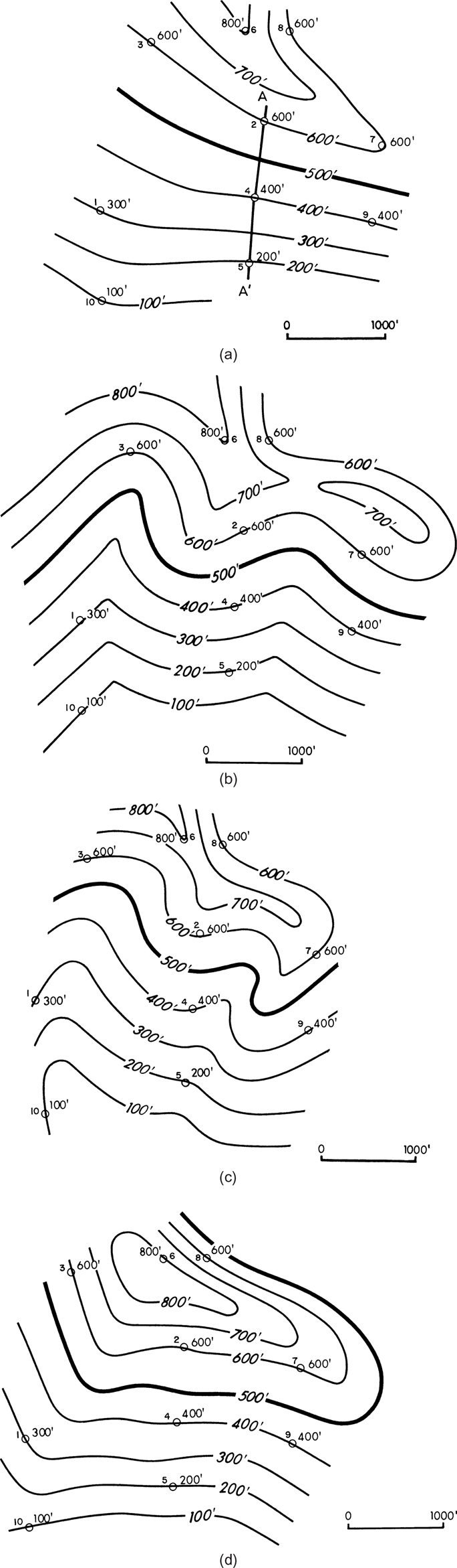
Figure 8-9 (a) Mechanical contouring method. (b) Equal-spaced contouring method. (c) Parallel contouring method. (d) Interpretive contouring method. (Modified after Bishop 1960. Published by permission of author.)
Parallel Contouring. With this method, the contour lines are drawn parallel or nearly parallel to each other. This method does not assume uniformity of slope or angle of dip; therefore, the contour spacing can vary. Like the previous method, if honored exactly, parallel contouring yields an unrealistic geological picture. It allows for some geological license to draw a map a little closer to the real world as there is no assumption of uniform dip (Fig. 8-9b).
Equal-Spaced Contouring. This method assumes uniform slope or angle of dip over an entire area or at least over an individual flank of a structure. Sometimes this method is referred to as a special version of parallel contouring. The advantage to this method, in the early stages of mapping, is that it can indicate the maximum number of structural highs and lows expected in an area of study (Fig. 8-9c).
Interpretive Contouring. With this method, the geoscientist has extreme geological license to prepare a map to reflect the best interpretation of the area of study, while honoring the available control. No assumptions, such as constant bed dip or parallelism of contours, are made. Therefore, the geoscientist can use his or her experience, imagination, ability to think in three dimensions, and an understanding and knowledge of the structural and stratigraphic styles of the geological region to develop an accurate and realistic interpretation. This method is the most acceptable and the most commonly used method of contouring (Fig. 8-9d).
The specific method or combination of methods chosen for hand-contouring may be dictated by such factors as the number of control points, the areal extent of these points, and the purpose of the map. No individual can develop an exact interpretation of the subsurface with the same accuracy as that displayed on a topographic map. What is important is to develop the most reasonable and realistic interpretation of the subsurface with the available data.
Contouring Faulted Surfaces
The contouring of faulted surfaces adds complications in the contouring of both structural horizons and faults. A completed structure contour map on one or more horizons is usually the main objective in any mapping project. In order to construct a completed structure map, however, the faults themselves must be contoured and the fault surface maps integrated with the structure maps. This integration is required to support a reasonable geological interpretation and to prepare accurate maps. In terms of map accuracy, this integration does the following (see Fig. 8-10):
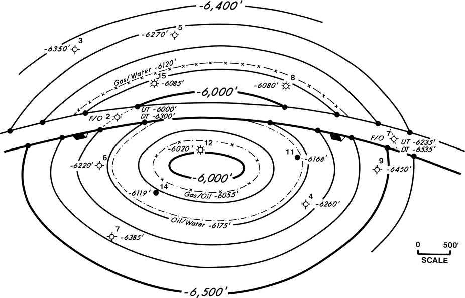
Figure 8-10 Integrated fault and structure map for the 6000-ft Horizon. The darkened circles delineate the intersection of each structure contour with the fault contour of the same elevation.
Delineates the position of the footwall (upthrown) and hanging wall (downthrown) cutoffs or traces of the fault in map view
Provides for the proper contouring of the mapped horizon across the fault
Depicts the vertical separation of the fault for any particular mapped horizon
Defines the limits of fault-bounded reservoirs
Fault surface mapping is covered in detail in Chapter 7. In this section, we present the proper techniques for integrating a fault surface map with a structure contour map. Included in this section are (1) techniques for positioning the upthrown and downthrown traces of a fault on a structure map; (2) construction of the fault gap or overlap; (3) the mapping of vertical separation versus throw; (4) the use of restored tops in structure mapping; (5) the application of contour compatibility across faults; and (6) the exceptions to contour compatibility.
Techniques for Contouring across Normal Faults
A fault trace is a line that represents the intersection of a fault surface and a structural horizon; it is sometimes referred to as a fault cutoff. Two fault traces (lines) are normally required to delineate a fault on a structure map. One line represents the footwall cutoff, or upthrown trace, and the other line represents the hanging wall cutoff or downthrown trace of the fault. Two conventions have been designed to indicate the direction of fault dip: (1) some type of symbol, like a “tent” or triangle, on the hanging wall cutoff (downthrown trace), and (2) the downthrown trace is heavier or thicker than the upthrown trace. The structure map in Figure 8-11a shows a fault displacing a contoured surface, using the conventional symbols described. It is important that all mappers at a given company use the same convention and use it consistently. This will aid managers in quickly reviewing maps from different individuals and subsurface teams. This issue is especially important when mapping on a computer, as computer software does not generally distinguish between the footwall and hanging wall traces.

Figure 8-11 (a) Faulted structure map on the 8000-ft Horizon. The structure is cut by a 400-ft fault. The correct method for contouring vertical separation (missing section) is illustrated by the dashed contour lines. (b) Fault surface map for Fault 1, which strikes east-west and dips at 50 deg to the south. (Published by permission of D. Tearpock.)
The techniques presented in this section demonstrate the correct method for projecting established contours from one fault block across a fault into another fault block. Using the available data (Fig. 8-11a), contours are first established for the block with the best control, which in this case is the upthrown block with four wells. These contours are extended to the upthrown trace of Fault 1. To contour across the fault, project the contours from the upthrown block through the fault into the downthrown block. This is shown in Figure 8-11a by a set of dashed contour lines continued across the fault gap indicating what the structural attitude of the horizon would be if the fault were not there. In other words, where would the contours be drawn if the fault were not there? Once the contours are projected through the fault gap to the downthrown fault trace, they are adjusted relative to the upthrown contour values by using the amount of vertical separation, which in this case is 400 ft. The downthrown block is then contoured. For example, the −8400-ft contour in the upthrown block, when projected into the downthrown block, becomes the −8800-ft contour.
Contours may be projected for some distance within the fault gap. Notice how the −8300-ft contour is projected from the upthrown trace of the fault for some distance through the fault gap before it intersects the downthrown trace and enters the downthrown block as an −8700-ft contour. The mechanics of projecting contours, such as the −8300-ft contour, through the fault, as shown in this figure, is the correct technique for contouring across a normal fault, using the vertical separation as obtained from well log correlation (missing section) or seismic sections where there is contour compatibility across the fault. The application of this technique leads to correctly delineating the position of the upthrown and downthrown traces of the fault, thus establishing the fault gap. It also assures that the correct displacement has been mapped across the fault (Tearpock and Harris 1987; Tearpock and Bischke 1990).
Some of you may still be asking yourselves why throw was not contoured across the fault. One reason is that no throw data are available for mapping, and throw is not the correct vertical displacement we want to map across the fault (refer again to Chapter 7). However, if we want to know the fault throw and heave, their values can be determined by simple measurements once the structure contour map has been prepared, as shown in Figure 8-11a or by use of Eq. (7-1a).
Throw is the difference in the vertical depth between where the fault intersects a specific horizon in the upthrown block and where it intersects that same datum in the downthrown block, measured perpendicular to the strike of the fault surface (not perpendicular to the strike of the fault trace). Therefore, a fault surface contour map must be available in order to calculate the throw from a completed structure contour map, as shown in Figure 8-11a. The fault shown in Figure 8-11b strikes east-west; therefore, the throw is determined in a north-south direction (see arrows in fault gap through Well No. 7). Using the points A and B on the map (Fig. 8-11a), the upthrown depth at point A is −8465 ft and the downthrown depth at point B is −8940 ft. The throw of the fault at this location is the difference between these two depths, or 475 ft.
We can calculate the throw mathematically by applying Eq. (7-1a), and knowing that the missing section in Well No 7 is 400 ft, the apparent bed dip, that is, the bed dip perpendicular to the strike of the fault, is about 10 deg at point A, and the fault dip is 50 deg. Equation (7-1a) yields a ratio of vertical separation (AE) to throw (AC) of 0.85, the absolute value of [(tan10 deg/tan50 deg) − 1]. The throw is thus (400 ft/0.85), or 470 ft. Considering the accuracy of graphical measurements on a contoured map, these two estimates for throw are in excellent agreement. We can see for this particular example that the throw is about 70 ft greater than the vertical separation.
Heave, which is the horizontal distance across the fault gap from the upthrown to downthrown traces, measured perpendicular to the strike of the fault surface (not perpendicular to the fault trace), is 390 ft. Therefore, a fault surface map must be available to determine heave as well.
For subsurface petroleum-related structure mapping, the measurements of throw or heave are usually measured for academic purposes and have little application in the actual contouring of a structure map. However, the throw and heave can be used to check a completed structure map using the graphical and mathematical methods described in this chapter and in Chapter 7. If the estimates for throw or heave determined by both methods (graphical and mathematical) are reasonably close, you can conclude that the map construction is reasonable. We point out here that the mapping of throw and heave are important in subsurface mining, the mapping of subsurface mineral deposits and outcrop mapping.
To further illustrate the proper construction of contours across a fault, we review Figure 8-12, using the same data given in Figure 8-11, with one exception. In this case, we map a horizon about 2000 ft shallower, and at this level the fault trace falls on the northern flank of the structure. Here the fault is dipping in the opposite direction as the horizon. The horizon, dipping generally to the north, is displaced by the south-dipping fault. The fault has a vertical separation of 400 ft. From the data points available, the structure contours were first established in the upthrown block and extended to the upthrown trace of Fault 1. As shown in the figure, to contour across the fault it is necessary to project the contours from the upthrown block through the fault gap to the downthrown trace of the fault, and then into the downthrown block. Ask yourself where the contour would be drawn had the structure not been faulted. The construction from one block to the other is shown by a series of dashed contour lines placed from the upthrown trace, through the gap, to the downthrown trace. Once the contours have been projected into the downthrown fault block, they are adjusted in depth from the upthrown contour values by the amount of vertical separation, which in this case is 400 ft. As an example, the −6000-ft contour in the upthrown block projected into the downthrown block becomes a −6400-ft contour. As in Figure 8-11, the same technique is followed for construction of all structure contour lines.
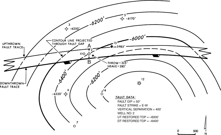
Figure 8-12 Portion of the structure map for the 6000-ft Horizon, showing the method for contouring vertical separation across a fault. (Published by permission of D. Tearpock.)
Now that the structure contours have been established in both blocks, the fault throw and heave can be calculated and measured. We graphically determine the throw of the fault by estimating the upthrown and downthrown structural depths using points A and B on the map. Notice that the values for throw and heave are different than those estimated in Figure 8-11a. The value for throw is now 325 ft, as compared with 475 ft in Figure 8-11a. The value for heave is 280 ft, as compared with 390 ft in Figure 8-11a. It is important to note that although the vertical separation does not change, there is a difference in the values for throw and heave. The missing section due to the fault has not changed, as it is equal to vertical separation and not throw. Remember, throw and heave are dependent fault slip variables that change with variation in the apparent attitude of the fault or horizon. In this case (Fig. 8-12), the fault intersects the horizon where the horizon dip is generally in the opposite direction to that of the fault. At the map level shown in Figure 8-11a, the fault and horizon are dipping in the same general direction. It is this change in relative dip direction (fault strike is unchanged) that causes the different values for throw and heave shown in the two figures, even though the vertical separation has not changed. Using Eq. (7-1a) and the data on the map near Well No. 2 (average bed dip is 14.5 deg), estimate the throw across the fault at points A and B and compare this estimate with that obtained graphically from the map.
Mapping Throw across a Fault.
Previously, we mentioned that missing section and repeated section due to a fault are equal to vertical separation. Let us assume for a moment, however, that a geoscientist incorrectly considers the fault data as throw and contours across the fault as if the missing section were throw. In Figure 8-13, the fault and structural data are exactly the same as that in Figure 8-11; therefore, we can compare the results of this (throw-contoured) map with the map in Figure 8-11a.
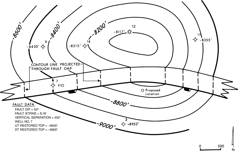
Figure 8-13 Fault and structure data are the same as shown in Figure 8-11a. For this interpretation, the missing section is contoured across the fault incorrectly as if it were throw. Compare the downthrown fault block with that shown in Figure 8-11a. (Published by permission of D. Tearpock.)
Using the available data, the contours are first established in the upthrown fault block and extended to the upthrown trace of Fault F-1. When contouring throw across a fault, the strike direction of a contour changes at this point and becomes perpendicular to the strike of the fault surface (Fig. 8-13). The contour is then projected through the fault gap to the downthrown trace of the fault. The strike direction of the contour is again changed to conform to its trend in the upthrown block.
Follow the −8500-ft contour through its construction in order to gain a good understanding of the technique. The strike direction of the −8500-ft contour in the upthrown block is established by the surrounding well control. At the intersection with the upthrown trace of the fault, the strike direction of the contour line changes abruptly to a strike direction that is perpendicular to the strike of the fault surface. In this example, as in the one in Figure 8-11a, the strike direction of the fault surface is east-west. Therefore, treating the vertical separation as if it were throw, the contour is projected through the fault gap in a north-south direction, perpendicular to the strike of the fault surface. At the intersection of the contour and the downthrown trace of the fault, the contour strike direction changes again to conform to the strike direction in the upthrown fault block. Once the contour is projected into the downthrown fault block, its depth is adjusted from the upthrown contour value by the amount of missing section (or in this case, assumed throw) of the fault (400 ft), so it becomes a 8900-ft contour.
A proposed well location is in the downthrown fault block in Figs. 8-11a and 8-13. Considering the correctly contoured map (Fig. 8-11a), the depth at which the proposed well is estimated to penetrate this horizon is −8720 ft, whereas at the same location on the incorrectly contoured map (Fig. 8-13), the well is estimated to penetrate the horizon at −8640 ft. The depth to the horizon is mapped 80 ft shallower on the incorrect map. Contoured depth differences of 80 ft can make the difference between a successful well and a dry hole, or result in a well that is not drilled in the optimum position on the structure.
Based on the nature of this erroneous contouring technique (mapping vertical separation incorrectly as throw), the magnitude of error becomes greater near or on the crest of a structure, as well as becoming larger with increasing structural dip. This is very critical since hydrocarbons are often trapped near the crest of structures and we commonly map these areas.
Over the years, we have reviewed hundreds of maps that have been contoured incorrectly as shown here. This is a common error based on a misconception of the meaning of throw. This error has caused petroleum companies hundreds of millions of dollars in dry holes or poorly positioned wells. The information presented here should provide you the basic knowledge needed to avoid similar or costly errors (Tearpock et al. 1994). Furthermore, good field training in which maps are made on faulted structures using outcrop and well log data can provide the 3D understanding of these various fault components, their important differences, and the impact of mapping vertical separation incorrectly as if it were throw.
Error Analysis—Procedure for Checking Structure Maps.
The best way to check whether a map has incorrectly used vertical separation as throw is to determine the vertical separation on the map by projecting the contours through the fault gap, as illustrated in Figure 8-11a and comparing it with the missing section in nearby wells. The missing section in Well No. 7 in Figure 8-11a is 400 ft. This matches the vertical separation shown by the map in Figure 8-11a. The missing section in Well No. 7 in Figure 8-13 is still 400 ft, but the vertical separation determined from the map in Figure 8-13 by projecting the upthrown −8500-ft contour through the fault gap to line up with the downthrown −8800-ft contour is 300 ft (Fig. 8-13). The lack of agreement between the missing section in the well and the vertical separation determined from the map demonstrates that the map in Figure 8-13 is incorrect. Without knowledge of the missing section in a well or the vertical separation measured from a seismic line, there is no way to know whether the map in Figure 8-11a was correct or the map in Figure 8-13 was correct.
The values for the vertical separation, fault dip, and bed dip can be determined from normal mapping parameters. With these data, Eq. (7-2) can be used to calculate the throw at any point along a fault. If the calculated value for throw agrees fairly well with the value determined graphically from the map, we can conclude that the interpretation is reasonable. If the missing or repeated section were mapped as throw instead of vertical separation, the value for throw determined mathematically will not compare favorably with that determined graphically, indicating that the map is in error.
The graph presented in Figure 8-14, which is derived from Eq. (7-1a), can be used during daily operations to check the consistency of structure contour maps and to ensure that a structure map has been contoured correctly across any existing faults. Equation (7-1a) is accurate for the situation in which the bed dip direction is more or less perpendicular to the strike of the fault surface (regardless of whether the beds dip toward the fault or in the same direction as the fault). So the graph in Figure 8-14, and also the graph in Figure 8-16, should be applied to that structural condition. That relationship is common in prospective closures against faults, and prospects are where you most want to check the accuracy of structure maps. For structural configurations where true bed dip is not perpendicular to the strike of the fault, use apparent bed dip measured perpendicular to the strike of the fault.
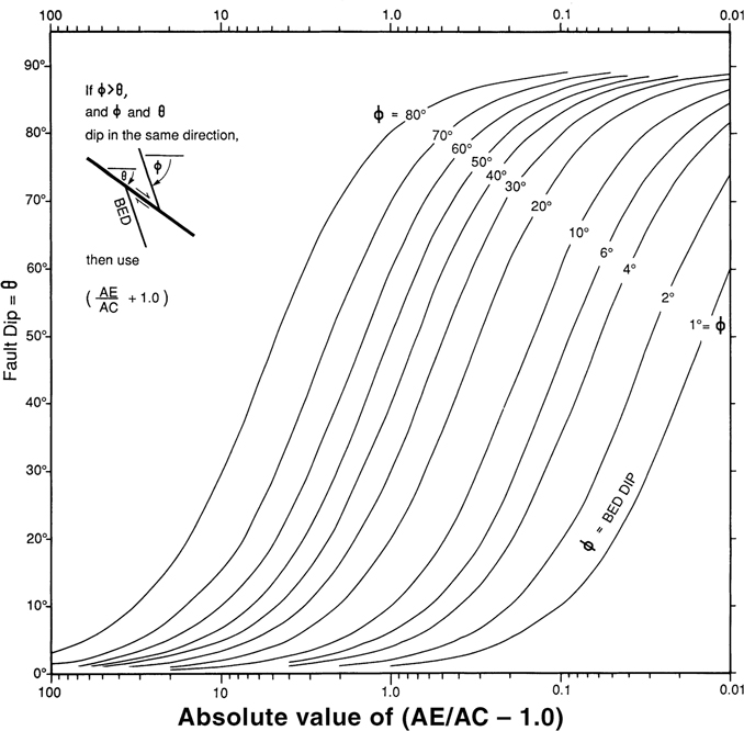
Figure 8-14 Graph used to check contouring across a fault. See text for explanation. (Published by permission of D. Tearpock and R. Bischke.)
In Figure 8-14, the fault and bed dips are taken to be clockwise. If the beds and fault dip in the same direction, the ratio AE/AC (vertical separation/throw) must be added to 1.0 in the figure. This is the case of a repeated section due to a normal fault.
As a practice exercise, use the data in Figure 8-11a, near the proposed location, and the graph (Fig. 8-14) to verify the dip of Fault 1 shown in Figure 8-11b.
An example of how to use Figure 8-14, for steeply dipping beds encountered around a salt dome, is as follows. On Figure 8-14 the fault dip θ is on the y-axis, the bed dip ϕ are the dipping lines in the central portion of the graph, and the absolute value of (AE/AC − 1.0) is plotted on the x-axis. Assume a fault has a dip of 50 deg. If the vertical separation AE is 400 ft and the throw AC is 200 ft, then the ratio of AE/AC = 2.0. The absolute value of (AE/AC − 1.0) = 1.0. Next, construct a vertical line from the abscissa of Figure 8-14 at the value of 1.0 and a horizontal line, across the graph from the ordinate, for a fault that dips at θ = 50 deg. The two lines cross the steeply dipping bed-dip curves at about ϕ = 50 deg. Thus, a correctly contoured map is consistent with a bed that dips at 50 deg into a fault that also dips at 50 deg (in opposite directions), for a vertical separation of 400 ft and a throw of 200 ft.
The relationship shown in Figure 8-15 is used to conduct error analyses on incorrectly contoured maps (i.e., how much error is introduced into a map that assumes the missing or repeated section in a well is throw). By this time it should be readily apparent that if vertical separation is mapped as if it were throw, the errors involved could result in a well that totally misses its target. The graph in Figure 8-16, derived from the relationship in Figure 8-15, can be used to analyze the magnitude of error (Tearpock and Bischke 1990). Figure 8-15 illustrates a faulted horizon for which the footwall position is determined incorrectly by mapping vertical separation as throw. From Figure 8-15:
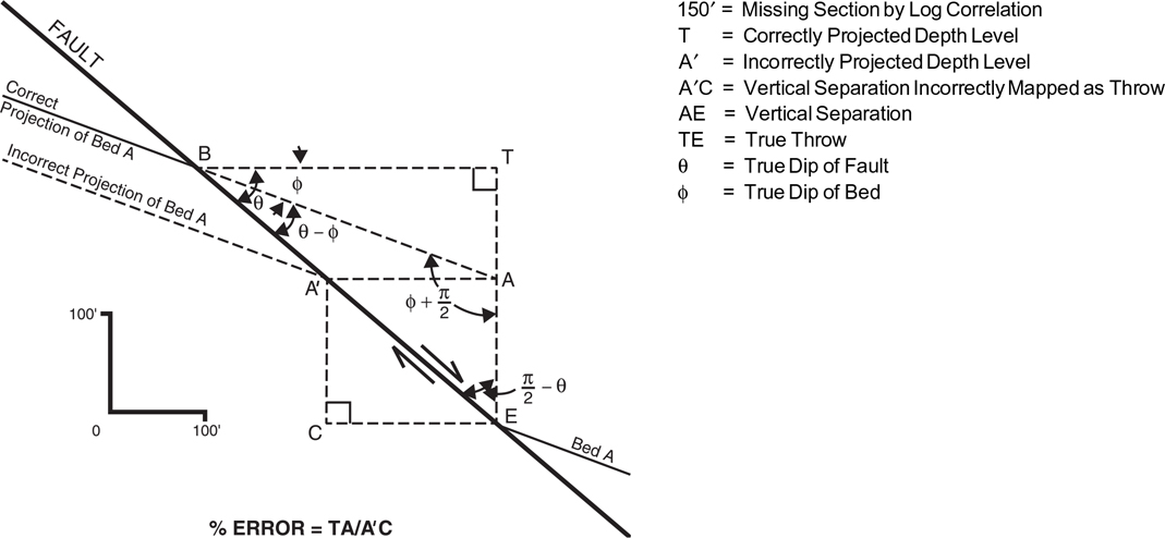
Figure 8-15 The relationship shown here can be used to conduct error analysis on incorrectly contoured structure maps. Based on the bed dip and intersection of Bed A and the fault in the downthrown block (hanging wall), observe the difference between the correct versus incorrect depth of intersection of Bed A and the fault in the upthrown block (footwall). Bed dip and fault dip are virtually in the same direction. (Published by permission of Tearpock and Bischke.)
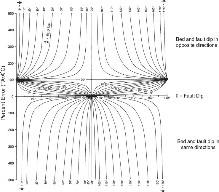
Figure 8-16 Graph used to measure the percent error on an incorrectly contoured structure map. Fault and bed dips are taken to be clockwise from 0 deg to 180 deg. (Published by permission of Tearpock and Bischke.)
Therefore, from the law of sines,
As

The distance TA is the error in depth between the correct (B) and incorrect (A′) points for the horizon projected onto the footwall. The ratio TA/A′C provides a percent error relative to the vertical separation value AE, which was incorrectly used as throw. Thus, Figure 8-16 can be used to measure the error that is introduced by improper contouring techniques.
On Figure 8-16 the percent error TA/A′C is plotted on the y-axis against the fault dip q on the x-axis. The bed dips f plot across the body of the graph as the gently to steeply dipping curved lines. The plot is symmetric across a horizontal line at which percent error = 0, to distinguish between beds that dip in the same direction of the fault (plotted on lower half of Fig. 8-16) from beds that dip in the opposite direction of the fault (upper half of plot). On the plot the errors range from 0% to 500%.
An examination of Figure 8-16 shows that unacceptably large errors of greater than 50% are introduced for faults dipping at angles of less than 30 deg (or greater than 150 deg) and for beds dipping at less than 5 deg (or greater than 175 deg, recognizing that 180 deg is a lower dip than 175 deg). For faults dipping at 45 deg, bed dips of 10 deg or more can introduce unacceptable errors. Notice that if the beds are dipping in the same direction as the fault, then the errors encountered are correspondingly larger (see lower half of the graph) than a situation in which the beds are dipping in the direction opposite to the fault. If the bed dip is about equal to the fault dip, as is often the case along the flanks of salt domes, then the errors involved in mapping vertical separation as throw can readily exceed several hundred percent.
In Figure 8-16, the error is relative to the depth of an incorrectly contoured horizon or a horizon mapped as throw. To calculate the error encountered when mapping vertical separation as throw, consider a bed dipping at 135 deg (or 45 deg to the west) into a fault that dips at 45 deg to the east. On the plot, a 45-deg fault dipping to the east is located along the 0% error line at 45 deg. From this value, project a vertical line from the x-axis into the upper portion of the plot. This portion of the plot defines beds that dip in the direction opposite to the fault. A bed dipping at 135 deg is located between the gently sloping 130-deg to 140-deg dipping lines (see X on plot). The percent error in incorrectly mapping a vertical separation as throw can now be determined by projecting the bed and fault dip intersection at X over to the y-axis.
Thus, a bed that dips at 135 deg (or 45 deg to the west) into a fault dipping at 45 deg (to the east) will have an error of 50%, which means that the correct depth to the bed under consideration is 50%, or one-half the vertical distance away from the incorrect level. Thus, relative to the correctly contoured bed, the error relative to the depth that should have been correctly contoured as vertical separation, is
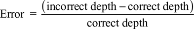
or

From this discussion, we can conclude that the errors involved in substituting throw for vertical separation are larger than most interpreters may realize or be willing to accept. Equations (7-1) and (8-1) and the graphs in Figures 8-14 and 8-16 are powerful tools that can be used on a daily basis to help generate correctly contoured maps and to evaluate the maps of others. Such analysis can be routinely conducted when evaluating prospect maps. Use Figure 8-16 to analyze the magnitude of error in the incorrectly contoured map in Figure 8-13, in the area of the proposed location.
The Legitimate Contouring of Throw.
The contouring of throw is a legitimate technique. Where all fault data are in terms of throw, such as in mining or outcrop geology, the construction of contours across the fault by mapping throw is an accepted technique. With regard to petroleum subsurface mapping, however, the technique is not valid, for most cases. First, well log fault data are not throw. Second, most seismic fault data given as throw are actually apparent throw. Third, if throw is measured from a seismic section, it cannot be tied to fault data from well logs for mapping, since measurements of fault displacement, using logs, are of vertical separation. Finally, throw often varies significantly along the strike of a fault; therefore, if throw is to be mapped, an almost infinite number of fault throw values are required to integrate a fault with a structure contour map.
When throw is the desired fault component to map, as in mining or outcrop mapping, the technique is sometimes incorrectly used. We shall look at one of the main errors made in mapping throw. Remember from previous discussions that true throw is measured perpendicular to the strike of the fault surface and not necessarily perpendicular to a fault trace shown on a structure map. Therefore, to project the structure contours through a fault gap, the fault surface map must be available to determine the strike of the fault. Since the strike of a fault can change across the mapped area, it is good practice when mapping throw to place the fault surface map under the structure map to obtain the strike direction of the fault so that all the contours can be projected through the fault gap perpendicular to the strike of the fault surface at any location along the fault.
At times, contours are projected through a fault perpendicular to the fault trace rather than the strike of the actual fault surface. This can result in serious mapping errors. If the strike directions of the fault itself and the fault trace are extremely close, the trace may be used to project contours with minimal error. But this is not always the case. The line of intersection between two inclined planes with different strikes (such as a horizon and fault) is not parallel to the strike of the horizon or the fault. Therefore, fault traces are normally not parallel to the strike of either the horizon or fault. Figure 8-17 shows such an example. The map in Figure 8-17 is contoured incorrectly by projecting the structure contours from the upthrown fault block through the fault gap perpendicular to the trace of the fault. In Figure 8-18, the contours are projected correctly through the fault gap perpendicular to the strike of the fault surface (see line indicating fault strike). Notice that the contour value of the point labeled X in the downthrown fault block is mapped 95 ft deeper using the incorrect technique. Depending on the amount of vertical separation and the difference in attitudes between the fault surface and horizon, the magnitude of contour errors on completed maps can vary from being insignificant to being very significant. When mapping throw, take the time to use the technique correctly.
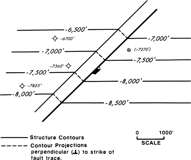
Figure 8-17 Structure contours illustrate the incorrect method for mapping throw perpendicular to the strike of the fault trace (see dashed contours in fault gap).
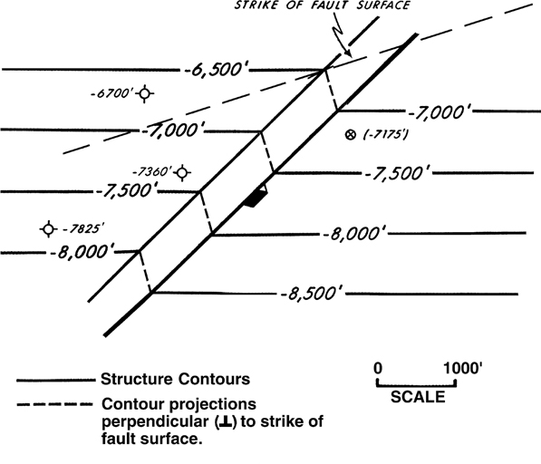
Figure 8-18 Structure contours illustrate the correct method for mapping throw perpendicular to the strike of the fault trace (see dashed contours in fault gap).
For petroleum geology mapping, you might consider this discussion on the correct technique for mapping throw as more of an academic exercise than one having some practical importance. But remember that in mining geology and outcrop mapping, where the actual fault surface can be touched and throw values physically measured, this mapping technique is valid. You should, however, consider one important point. If the fault data consist of both actual throw measurements from a mine or an outcrop, and well log fault data, they cannot be used together in structure mapping because the well log fault data represent vertical separation. Equation (7-1), however, can be used to convert the throw data to vertical separation, or vice versa, which can then be used for mapping.
Only if the dip of the horizon being mapped is zero or nearly so, or if the fault is vertical, are the values for vertical separation and throw essentially the same. In these cases, they can be used together in fault and integrated structure mapping.
Later in this chapter, we examine a petroleum-related generic case study, which further illustrates the importance of mapping the missing section correctly as vertical separation rather than as throw in petroleum subsurface mapping. It can make the difference between drilling a successful well and a dry hole.
Technique for Contouring across Reverse Faults
The technique presented for contouring across a normal fault is also applicable for contouring across a reverse fault. Reverse faults and overthrusts, however, produce a fault overlap rather than a fault gap. Figure 8-19 shows the technique for contouring across a reverse fault. The 4500-ft Horizon, which dips generally to the west-northwest, is displaced by a southwest-dipping reverse fault. The vertical separation or repeated section determined from well log correlation is 450 ft.
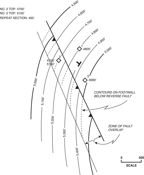
Figure 8-19 The correct method for contouring repeated section (vertical separation) across a reverse fault is illustrated by the solid and dashed contours in the fault overlap. This reverse fault has 450 ft of vertical separation (repeated section) as evidenced by the repeated tops in Well 2 that are 450 ft apart.
The technique for contouring across a reverse fault is usually easier than that for a normal fault because there is no projection of contours through a fault gap. With a reverse fault, the hanging wall is thrust up and over the footwall, resulting in an overlap of structural horizons. Therefore, the hanging wall is contoured right up to the hanging wall cutoff at the upthrown fault trace. Likewise, the footwall is contoured up to the footwall cutoff at the downthrown trace of the fault. Since the fault blocks overlap, the strike direction of the contours established in the block that is contoured first (the block with the most control) serves as a guide to the contouring of the other fault block. As with the normal fault example, to guide the strike direction of the contours, consider how the structure would be contoured if the fault were not there. Wells positioned in the fault overlap serve as a guide to the contouring of both fault blocks.
Referring back to Figure 7-29 in Chapter 7, the thickness of the repeated section or vertical separation resulting from a reverse fault can be calculated by measuring the vertical distance from the top of the mapped horizon in the hanging wall to the top of the same horizon in the footwall. Notice that Well No. 2 in Figure 8-19, in the fault overlap, has penetrated the top of this horizon twice: the first time at 4700 ft and the second time at 5150 ft. The vertical difference between these two tops is equivalent to the repeated section or vertical separation, which is equal to 450 ft. The vertical separation can therefore be seen directly in the fault overlap.
There is one problem with the construction of a reverse fault overlap; it results in significant clutter, which can be confusing. Some confusion is eliminated by dashing the contours on the footwall beneath the fault, within the zone of fault overlap, as illustrated in Figure 8-19. Another method of eliminating clutter is to pull the fault blocks apart and present each fault block separately. This is a good way to construct a structure map with a reverse fault, especially if hydrocarbons are present and isochore maps are required. The method is shown later in this chapter.
There is an additional complication in using a workstation to map structures cut by reverse faults. Consider Well No. 2 in Figure 8-19. This well contains two tops for the same horizon as it penetrated both the hanging wall block and the footwall block. Most computer software packages do not handle repeated section very well, neither repeated tops in a well nor repeated horizons on a seismic line. With most computer software packages, it may be necessary to map the hanging wall block separately from the footwall block. Digital control points can be added to the map if needed to ensure contour compatibility across the fault.
Manual Integration of Fault and Structure Maps
In this section, we present the technique for manually integrating a fault surface map with a structural horizon map. The correct application of this technique is essential for accurate structure mapping in faulted areas. The technique provides the following important contributions to the structure contour map interpretation.
An accurate delineation of the fault location for any mapped horizon;
The precise construction of the upthrown and downthrown traces of the fault;
The correct width of the fault gap or overlap; and
The proper projection of structure contours across the fault based on fault data (vertical separation) from well logs or seismic sections.
Normal Faults
The step-by-step method of integrating a fault surface map of a normal fault with a structural horizon map is illustrated in Figures 8-20 and 8-21. Figure 8-20 is a fault surface map constructed from fault data from the wells shown on the figure. The fault strikes generally north-south, is slightly convex to the east with a dip of 45 deg, and has a vertical separation of 400 ft. The stratum being contoured is called the 7000-ft Horizon. The subsea tops for this horizon in each well are shown on the partly completed structure map in Figure 8-21a. In Well No. 3, for example, the top of the 7000-ft Horizon is at a depth of −7045 ft.

Figure 8-20 Fault surface map for Fault A constructed from well log fault data from seven wells. The fault map has a 1000-ft contour interval.

Figure 8-21 (a) Partially completed structure map on the 7000-ft Horizon. (b) Integration of the fault and structure maps to identify the intersection of the fault surface with the upthrown fault block of the 7000-ft Horizon. (c) Structure map shows the delineation of the upthrown trace of Fault A and the projection of form contours into the downthrown fault block. (d) Integration of the fault and structure maps to identify the intersection of the fault surface with the downthrown fault block of the 7000-ft Horizon. (e) The final, integrated structure map for the 7000-ft Horizon.
The 7000-ft Horizon is cut by Fault A. A review of the depth of the fault picks and the structure tops for each well indicates that five of the seven wells are in the upthrown block and that only Wells No. 4 and 5 are in the downthrown fault block. For a structure cut by a normal fault, wells in which the fault cut is above the structure top are in the upthrown (footwall) block and wells in which the structure top is above the fault cut are in the downthrown (hanging wall) block, unless the well drills the fault “backwards” and penetrates the fault from the upthrown (footwall) into the downthrown (hanging wall). Employing the general contouring guideline of beginning the structure contouring in the area or fault block with the most control, the contouring of the 7000-ft Horizon originates in the upthrown fault block. The initial contouring indicates an anticlinal structure with a slightly elongated east-west axis (Fig. 8-21a). The contours are not continued across the entire map area because at some point the contours in this upthrown fault block intersect Fault A and terminate at the upthrown fault trace. By underlaying the fault surface map beneath the structure map, the approximate location of this intersection can be determined and the contouring stopped in the vicinity of this intersection.
When doing this method by hand, the next step is to overlay the structure map (Fig. 8-21a) onto the fault map (Fig. 8-20), as shown in Figure 8-21b, to determine the upthrown trace of the fault. The upthrown trace occurs where structure contours in the upthrown block intersect fault contours of the same elevation. These intersections are highlighted on the map by a small mark placed at the end of each contour line, as shown in the figure. Because the fault surface map has a contour interval of 1000 ft and the structure contour map has a 200-ft contour interval, the precise position of the intersections for each contour line should be located by interpolation, using 10-point proportional dividers or a scale. Dividers or a scale allow subdivision of the 1000-ft fault contours into 200-ft intervals anywhere on the map without the clutter of actually drawing the extra contours (see Fig. 2-11). For a small portion of the fault map, 200-ft contours are shown between the −7000-ft and −8000-ft depths. These contours serve two purposes: (1) to illustrate the accuracy of the intersection of the fault and structure contours for the −7000-ft, −7200 ft, −7400-ft, −600-ft, −7800-ft, and −8000-ft elevations; and (2) to show that the construction of 200-ft fault contours over the entire map would result in unnecessary clutter. Two-hundred-foot (200-ft) contours can, however, be placed as marks in localized areas, as shown in the figure, to determine the intersections precisely. Once used for this purpose, the additional contours are then erased. After all the intersections have been identified, the upthrown trace of the fault is accurately constructed simply by connecting all the marks with a smooth line, as shown in Figure 8-21c.
The next step is to project the structure contours through the upthrown trace of the fault into the downthrown fault block. There are two points of control in the downthrown fault block that must be honored: the horizon elevation in Well No. 4 is −8420 ft, and in Well No. 5 it is −8130 ft. Earlier in this chapter, we presented the technique for projecting contours from one fault block across a fault into the adjacent fault block. This technique is used to complete the construction of the anticline in the downthrown fault block and delineate the downthrown trace of the fault. An easy way to remember the technique to guide your contouring through the fault is to consider how the structure would be contoured if the fault were not there. One method is to restore the faulted block to an unfaulted condition and relabel the depth values in the wells to account for the restoration. The unfaulted structure can then be mapped. Once completed, the map can be refaulted or restored again to its faulted condition. The structure contours must be adjusted again in consideration of the vertical separation. This is a time-consuming task when done by hand, whereas computers are more capable of using such methodology. For simplicity, often it is best to project the contours into the opposing fault block as form contours (contours without values) in order to complete the structural picture, as shown in Figure 8-21c.
Once contours are projected through the fault into the downthrown block, their values are adjusted from those in the upthrown block by the amount of vertical separation, which in this case is 400 ft. Thus, the projection of the −7400-ft contour from the upthrown block becomes a −7800-ft contour in the downthrown block. Continue this procedure for all contours projected through the fault. In Figure 8-21d, the downthrown contours have been assigned structural elevation values and now the downthrown trace of the fault can be determined. Again, the fault surface map is placed under the structure map and the intersections of the structure contours in the downthrown block with the fault contours of the same elevation are identified and indicated by small marks.
Finally, connect all the marks with a heavy smooth line to accurately delineate the downthrown trace of the fault. Place a symbol on the downthrown trace to show the direction of fault dip, erase the contours in the fault gap, and the integrated structure contour map for the faulted anticlinal structure is complete (Fig. 8-21e). By correctly integrating the fault and structure maps, we have (1) accurately delineated the position of the fault trace on the structure for a particular horizon; (2) precisely constructed the upthrown and downthrown traces of the fault; (3) established the actual width of the fault gap; and (4) projected the structure contours correctly across the fault. An understanding of this technique is paramount to the correct and precise integration of a fault map and a structure map; therefore, take the time to review and master this process.
For the example shown in Figure 8-21, the process was relatively easy because the structural pattern is a simple anticline cut by only one fault. But the procedure is basically the same for a more complex structure and pattern of faults. Figure 8-22 shows the complexly faulted anticlinal structure of an oil and gas field. A fault surface map was prepared for each of the 13 individual normal faults, and the integration technique was used to prepare the completed structure map. With a complex structure such as the one shown here, the logistics are more involved and it takes more time to prepare the fault maps and integrated structural interpretation, but the methodology is basically the same.

Figure 8-22 An integrated structure map of a very complexly faulted anticlinal structure. Each fault was integrated with the structural interpretation as shown in Figure 8-21.
Some software packages allow a geoscientist to create a surface from a horizon in a fault block and a surface from a fault interpretation. These software packages allow the horizon surface to be projected to or clipped at the fault surface. The intersection of these two surfaces forms a fault trace.
If the software package you are using does not allow you to create an intersection of the horizon surface and the fault surface, you can use the same procedure used for mapping a faulted structure by hand. First, create a polygon on your horizon map that roughly corresponds to the fault gap. Second, contour both the horizon and the fault. Third, display both the horizon contours and the fault surface contours on the screen at the same time. Fourth, adjust the polygon to match the intersection of the horizon contours in the fault block where you have the best data with the fault surface contours. As you are likely to use different contour intervals for the horizon and the fault surface, you will have to interpolate between fault contours, just as you would if contouring by hand. Fifth, adjust the horizon contours in the other fault block to reflect contour compatibility and the vertical separation of the fault, if necessary. Finally, display both the horizon and fault surface contours again and adjust the polygon so that it ties the intersection of the horizon and fault surface contours.
The details of how to accomplish these methods of integration with the various workstation programs are beyond the scope of this book. Chapter 9 on 3D seismic interpretation provides some additional guidance for this method in a general sense. Each geoscientist must learn the individual mapping program being used and determine the best method for combining the use of applications within each package in order to achieve this type of subsurface integration accuracy.
Restored Tops—An Aid to Structural Integration.
In Chapter 4 we mention that in dealing with normal faults, a given horizon or marker being mapped may be faulted out of one or more wells in the area of study. It is often possible, however, to estimate an upthrown and downthrown restored top for any horizon missing from the faulted well(s). A restored top is an estimated elevation for a specific marker or horizon that is faulted out of a well. In other words, a restored top is an estimate of the depth of a marker or horizon in a given fault block were it not faulted out of the well. The procedures for estimating restored tops for both straight and deviated wells were discussed in detail in Chapter 4. In Chapter 7, we also showed the importance of restored tops in estimating the amount of vertical separation for a growth fault.
In this section, we discuss how these restored tops are used to provide additional control points for fault and horizon map integration. Referring again to Figure 8-10, notice that the horizon is faulted out in Wells No. 2 and 7 and that estimated restored tops are indicated next to each well. For Well No. 2, the upthrown restored top (UT) is −6000 ft, and the downthrown restored top (DT) is −6300 ft; for Well No. 7, the UT is −6235 ft and the DT is −6535 ft. The vertical difference between DT and UT restored tops should be equal or nearly equal to the section missing in the wells due to the fault. In this case, the difference is 300 ft, which is equal to the missing section determined by log correlation; consequently, the restored tops appear consistent with the available data.
Procedures for projecting contours through a fault and the integration of a fault map with a structure map have been discussed, so we can review the structure map in Figure 8-10 and determine the amount of missing section. A darkened circle marks the intersection of each structure contour with the fault surface contour at the same elevation. By connecting these marks, the upthrown and downthrown fault traces are delineated as shown on the map. Any contour may be taken from its intersection with the upthrown fault trace and projected through the fault to the downthrown trace to estimate the vertical separation for the fault at this horizon. For example, the −6100-ft contour in the upthrown block projected through the fault gap intersects the −6400-ft contour in the downthrown block, indicating the fault displacement (vertical separation) of 300 ft, which was based on the restored tops and used in the mapping. The restored tops in Wells No. 2 and 7 provide important control points for contouring the structure map.
Restored tops are located in a vertical well itself (Fig. 4-42), or vertically above and below the fault pick in a deviated well (Fig. 4-43). They are not placed at the upthrown and downthrown traces of a fault. Using Figure 8-10 as an example, the restored tops for Wells No. 2 and 7 are placed right at the well locations. The dashed lines through each of the two wells illustrate the honoring of the restored tops in the wellbores. In Well No. 7, an interpolated contour of −6235 ft projects from the upthrown fault block into the well, and an interpolated contour of −6535 ft projects from the downthrown fault block into the well. Similarly for Well No. 2, the −6000-ft contour in the upthrown block and the −6300-ft contour in the downthrown block project into the well.
How are these restored tops used as an aid in structure mapping? Depths for restored tops are honored in the same way as any other well control point during structure mapping. For example, the UT restored top for Well No. 2 is −6000 ft; therefore, the −6000-ft structure contour in the upthrown block honors this control point at Well No. 2. Likewise, the −6300-ft contour in the downthrown fault block is projected through the fault gap to intersect with Well No. 2, whose DT restored top is −6300 ft. Each UT and DT restored top provides two additional points of control to aid in structure contouring in and around a fault. The contouring of the structure map in Figure 8-10 confirms that the four restored tops were used as control points in the construction of the final structure map.
In areas of limited well control, restored tops in faulted wells provide significant structural information which is often necessary for the preparation of a realistic and accurate structure map. Considering the well control in Figure 8-23a, how would you contour these data points? The data can be contoured in a number of ways. Figure 8-23b shows one interpretation which appears to be reasonable. The map does honor all the established well control and was used to propose the two drilling locations shown on the map. The first location is upthrown to Fault C in Reservoir C-3. An oil show in Well No. 14 establishes the down-dip limit of oil at −9245 ft. The proposed well is designed to penetrate the reservoir in the optimum position for maximizing the well’s drainage efficiency. Based on this interpretation, the volume of anticipated recoverable oil up-dip of the oil/water contact is 6480 acre-feet. Considering a reasonable recovery factor for this area of 450 barrels per acre-foot, this prospect represents 2,916,000 barrels of potentially recoverable oil. Downthrown to Fault C, a development location is proposed to maximize the drainage efficiency for the east-west elongated Reservoir C-5. Based on this structural interpretation, the volume of estimated reserves is 1,107,000 barrels of recoverable oil.
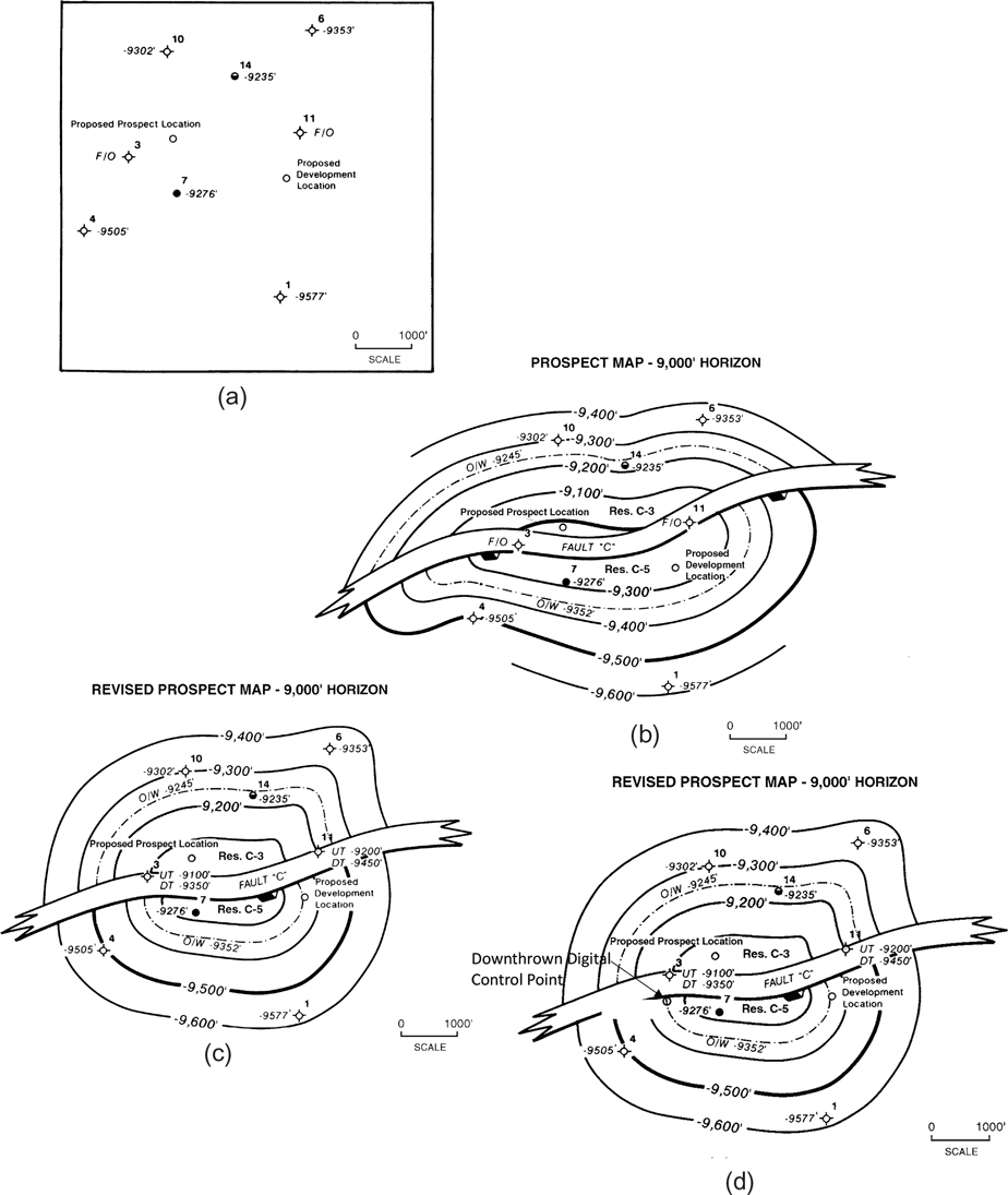
Figure 8-23 (a) Basemap with posted data for the 9000-ft Horizon. How would you contour the data? (b) Structural interpretation of the 9000-ft Horizon using all the well data except for the restored tops in Wells No. 3 and 11. Two development wells are proposed based on this interpretation. (c) Revised structural interpretation of the 9000-ft Horizon using all the available well data including the restored tops for Wells No. 3 and 11. Compare this interpretation with that shown in Figure 8-23b. (d) Revised structural interpretation with the DT restored top from Well No. 3 plotted just outside the fault gap as a digital control point for contouring on a computer. This figure illustrates only a single digital control point. When contouring on the computer, digital control points for both upthrown and downthrown restored tops would be used for both Well No. 3 and Well No. 11. Digital control points could also be used to project contours across the fault gap and constrain contouring of the downthrown fault block. (Figure 23d published by permission of J. Brenneke.)
The interpretation appears reasonable except for the two wells within the fault gap in which the 9000-ft Horizon has been faulted out. For whatever reason, no restored tops were estimated for these wells to incorporate into the structural interpretation. Figure 8-23c is a structure contour map for the same two reservoirs using the UT and DT restored tops for the 9000-ft Horizon in Wells No. 3 and 11 in the interpretation. It is obvious that the four restored tops are very important data needed to develop a more accurate interpretation of this structure. The addition of the restored top data has a significant impact on the interpretation of the overall geometry of the structure and the proposed well locations. For the upthrown Reservoir C-3, the volume of recoverable hydrocarbons has been reduced to 3480 acre-feet or 1,566,000 barrels of recoverable oil, a reduction in volume of 46%. The map for Reservoir C-5 in the downthrown block, using the restored tops, indicates that the volume of Reservoir C-5 is smaller by 41% compared to the map in Figure 8-23b. Potentially recoverable hydrocarbons decrease from 1,107,000 barrels to 648,000 barrels. More important, the proposed development location for Reservoir C-5 is actually down-dip of the oil/water contact, and if drilled, the well would result in a dry hole.
Information provided by the UT and DT restored tops was critical in this example. The tops are valuable mapping data that should not be ignored, particularly in areas of limited well control. These extra data points guide the structure contours into and through the fault gap. Figure 8-23 makes this point very clear. Upthrown and downthrown restored tops improve the accuracy of a structure contour map, and in this case reduced the size of the two prospective reservoirs.
Restored tops are also helpful in generating prospects where none previously existed. Figure 8-24a shows a portion of a structure contour map showing a potential oil reservoir. Notice Well No. 22 in the western portion of the map, upthrown to Fault A, has an oil show with an oil/water contact at 6458 ft TVD (true vertical depth). Well No. 25 to the east is wet and the mapping horizon is faulted out in Well No. 65 by Fault A. Based on the structural interpretation shown in this figure, the volume of potentially recoverable oil is insufficient to justify the drilling of an up-dip development well into Reservoir A-1. The structural closure is too small, and the target area between the oil/water contact and the upthrown trace of the fault too small to risk the drilling of a well. During the preparation of this structure map, the trace of Fault A was constructed based on isolated fault data without the use of a fault surface map and without estimated restored tops for the faulted out Well No. 65.

Figure 8-24 (a) Structure map on the 6450-ft Horizon shows Reservoir A-1 of insufficient size to justify a development well. This map was constructed without the integration of a fault map, and the restored tops for Well No. 65 were not used. (b) Revised structure map on the 6450-ft Horizon, Reservoir A-1. The revised interpretation was prepared using the restored top data from Well No. 65 and the integration of the fault surface map for Fault A with the structural interpretation. Also, shallower and deeper structure maps were used to guide the structure contouring. Reservoir A-1 is now of sufficient size to propose a development well location.
The structure map in Figure 8-24b was constructed using a fault surface map for Fault A to integrate with the structure and to contour across the fault. The UT and DT restored tops for this horizon in Well No. 65 were calculated and used, and maps on shallower and deeper horizons, in which the tops in Well No. 65 were present, were also made. These additional mapping data change both the configuration of Reservoir A-1 and the volume of potentially recoverable hydrocarbons. This accurately integrated structure contour map delineates a reservoir of sufficient size (569,000 barrels of oil) and closure to be reevaluated as a potential development location. The UT and DT restored tops are used in Figure 8-24b to guide the strike direction of the contours into the fault and to honor the vertical separation, thus changing the structural configuration of the reservoir.
We cannot overemphasize the importance of using all available data when preparing subsurface maps of any type. Geoscientists always work with limited data, so to ignore or not use valuable data, for any reason, is unthinkable. Our job is to develop the most reasonable and accurate interpretation possible from available data. The use of upthrown and downthrown restored tops is a necessary part of preparing a structure contour map. The time required to estimate these tops and incorporate them into the integrated structural picture is minimal, but it can have a significant impact on the final interpretation, as shown in the examples presented.
It is relatively simple to use restored tops when contouring by hand, but it is more difficult to use them when contouring on a workstation. This difficulty is for three reasons. First, restored tops need to be named differently than tops that are actually seen in a well. If the top of the J Sand is being mapped, tops actually seen in a well may be labeled J_t, whereas an upthrown restored top might be labeled J_t_ut. We recommend that tops be named with the shortest reasonably descriptive name because top names can obscure features on a computer screen. The shorter the name, the less information is obscured. This issue can be solved fairly simply in most computer systems by telling the system that J_t_ut is an alias of J_t, so the software will treat the two tops as equivalent. Shorter names also slightly minimize the issue of multiple names for the same top. To a computer, the J Sand, J sand, J-Sand, and J_Sand are four unique tops.
This solution runs into the second difficulty in using restored tops on a workstation. Most software programs struggle if there are two tops of the same stratigraphic marker in the same well. A third problem arises because restored tops occur in the fault gap, which is usually represented on a workstation by a polygon within which data is excluded. Finally, some computer systems expect tops to be in a stratigraphic order. Restored tops can violate this order. These last three issues can be finessed by placing digital control points representing the restored tops just outside the exclusion polygon (Fig. 8-23d). These digital control points are placed by estimating where they would project outside the exclusion polygon to match contours projected into the exclusion polygon to tie the restored tops. It may be necessary to move these digital control points to make sure the contours project through the faulted out well and reflect contour compatibility across the fault.
Restored tops in deviated wells are a special challenge when mapping with a computer. As discussed in Chapter 4, restored tops are placed directly above and below the fault cut in a deviated well (Fig. 4-43). They are not placed at their subsea depth along the deviated well path. We are not familiar with any computer mapping system that plots restored tops correctly on deviated well paths, although there may well be such systems available. Go back and review Figure 4-43. If the upthrown restored top for Sand B is plotted on the directional path of Well No. 3, it will plot out of stratigraphic sequence as it will be above the upper marker. It will also plot outside of the fault gap in the downthrown fault block. This issue may be resolved by initially entering restored tops as digital control points at the X-Y position of the fault cut and later moving the digital control points outside the fault exclusion polygon once the form of the contours takes shape. We emphasize that placing restored tops as digital control points is an iterative process where their precise location is dependent on the final location of the structural contours and the integrated location of the fault traces.
Reverse Faults
The method of manually integrating a reverse fault surface map with a structure contour map is illustrated in Figures 8-25 and 8-26. We do not describe the procedure in as much detail as we did for the integration of normal faults, since the procedure is basically the same. There are seven wells from which fault and horizon data were obtained. Figure 8-25 shows the reverse fault surface map constructed using the data from the seven wells. The fault strikes generally north-south with a dip of 35 deg to the west and has a displacement (vertical separation) of 300 ft, as shown by the values of repeated section in the well data.

Figure 8-25 Fault surface map for reverse Fault 1 based on well control from seven wells. Depth values are positive, indicating they are above sea level.
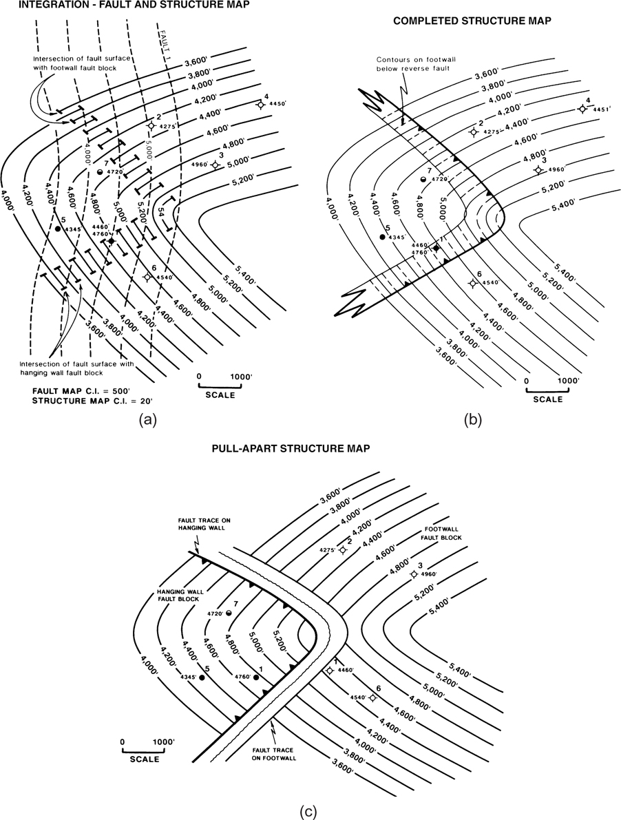
Figure 8-26 (a) The fault map is placed under the structural interpretation to obtain the intersection of the fault surface with both the footwall and hanging wall fault blocks. (b) Final integrated structure map for the 5000-ft Horizon. (c) A pull-apart map of the final integrated structural interpretation. This type map separates the footwall and hanging wall fault blocks to show them individually, without the clutter of overlapping contours.
The technique for integrating a reverse fault surface map with a horizon map is often easier than that for a normal fault because there is no projection of contours through a fault gap. In the case of a reverse fault, the hanging wall is thrust up and over the footwall, resulting in an overlap of structural horizons. Therefore, the hanging wall is contoured up to the hanging wall cutoff at the upthrown trace of the fault, and the footwall is contoured up to the footwall cutoff at the downthrown trace of the fault. Since the fault blocks overlap, the strike direction of the contours established in one fault block can often be used to guide the direction of the contours in the opposing block.
The faulted structure for this example (Fig. 8-26) is the nose of a plunging anticline that is penetrated by seven wells. Wells No. 2, 3, and 6 penetrated the footwall, Wells No. 5 and 7 penetrated the hanging wall, and Well No. 1 is in the fault overlap, thereby penetrating the horizon twice: first at 4760 ft in the hanging wall, and second at 4460 ft in the footwall. Notice that the contour values are positive, indicating this structure is above sea level.
We begin contouring this structure in the hanging wall fault block. Place the fault surface map under the structure map as shown in Figure 8-26a. The fault trace on the hanging wall occurs where the structure contours in the hanging wall intersect fault surface contours of the same elevation. These intersections are highlighted on the map as small marks placed at the end of each contour. Likewise, as we contour the footwall horizon, the fault trace is located where the structure contours in the footwall intersect fault contours of the same value. Again, these intersections are highlighted by small marks placed at the end of each contour (Fig. 8-26a). For accuracy, 10-point dividers or a scale may be used to locate the exact points of intersection between structure and fault contours.
The difference in elevation between contours in the footwall and those in the hanging wall equals 300 ft, which is the value of the vertical separation or repeated section determined from well log correlation. For example, the 4000-ft contour in the footwall within the zone of overlap is positioned directly under the 4300-ft contour in the hanging wall. This same 300-ft difference in contour elevation is maintained for each of the structure contours in the mapped area.
Finally, connect all the marks representing the intersections of the fault surface with the footwall and hanging wall structure contours with smooth lines to accurately delineate the fault traces (Fig. 8-26b). Place a symbol on the hanging wall fault trace to show the direction of fault dip and dash the structure contours in the footwall, under the fault overlap for clarity. Having completed these various steps, the integrated structure contour map for the faulted plunging anticlinal nose is complete.
By correctly integrating the fault and structure maps, the following is accomplished: (1) the position of the fault on the mapped horizon is accurately delineated; (2) the traces for the fault are precisely constructed; (3) the actual width of the fault overlap is established; and (4) the contours are carried correctly in the fault overlap. Although the actual fault surface map is striking north-south, the trace of the fault on this horizon strikes northwest-southeast on the northern flank of the structure and southwest-northeast on the southern flank of the structure. The curved shape and position of the trace for Fault 1 on this structure map could not be intuitively constructed without the integration of the fault and structure maps.
We mentioned earlier that a structure map with a reverse fault overlap is cluttered and can be confusing because of the double set of contours in the overlap. One way to minimize the clutter and confusion when contouring by hand is to dash the contours in the footwall in the zone of overlap (Fig. 8-26b). Another solution to the clutter and confusion is to prepare a pull-apart map, as shown in Figure 8-26c. With this map, the two separate fault blocks are pulled apart or mapped separately to show each block separately without any overlap. Such a map should be constructed only after the fault and structural integration is complete in order to eliminate any possibility of contouring errors. In this example, the hanging wall is productive of hydrocarbons. Eventually, net sand and net oil isochore maps will be constructed for the hanging wall reservoir. These maps can be prepared more easily if the fault blocks are separated as shown in Figure 8-26c.
There is an additional complication in using a workstation to map structures cut by reverse faults. Consider Well No. 1 in Figure 8-26. This well contains two tops for the same horizon, as it penetrated both the hanging wall block and the footwall block. Most computer software packages do not handle repeated section well, either with repeated tops in a well or with repeated horizons on a seismic line. With most computer software packages, it may be necessary to map the hanging wall block separately from the footwall block. Digital control points can be added to the map to insure contour compatibility across the fault.
Fault Traces and Gaps—Shortcuts and Pitfalls
The following discussion refers primarily to fault traces and gaps formed by normal faults; however, the geometric relations are also applicable to fault overlaps formed by reverse faults. Fault traces are the two lines on a structure contour map representing the intersection of a fault surface with the structure-contoured horizon in the upthrown and downthrown fault blocks. Together, the fault traces form the overall trace for a fault on any particular mapped horizon. Both fault gap and fault overlap are each defined as the horizontal distance between the upthrown and downthrown fault traces measured perpendicular to the fault traces, as depicted on a completed structure contour map. When the integration technique is used, the fault gap or overlap is automatically constructed, since it is the horizontal distance between upthrown and downthrown traces.
With regard to the trace of a fault and the resultant gap or overlap, there are some common misunderstandings that we intend to clarify. Also, we present some shortcuts for delineating fault traces and gaps, and the pitfalls associated with these shortcuts.
There is widespread belief that the horizontal width of a fault gap equals the amount of vertical separation, as obtained from well logs or seismic data. It is thought that the fault gap may therefore be scaled off, using the horizontal reference scale on the map. Thus, for a fault with 500 ft of vertical separation, the width of the fault gap could be mechanically constructed by scaling off a 500-ft Horizontal gap between the upthrown and downthrown traces of the fault, using an engineer’s scale or dividers. This technique is often incorrect and should be employed only under special conditions. The technique assumes that the positions of the upthrown and downthrown traces of the fault are known. However, fault trace positions are very difficult to define without the use of the fault/structure map integration technique. The width of a fault gap is also a function of the strike and dip of the fault, as well as the strike and dip of the horizon. Therefore, on a single structure contour map, variations in the attitude of either a fault or the horizon may result in changes in the width of the fault gap from place to place, although the vertical separation for the fault itself has not changed.
There is a general rule that should be kept in mind regarding fault gap. A fault dipping in the opposite direction of bed dip will have a narrower fault gap than a fault (with the same displacement) dipping in the same direction as the bed dip. Look again at Figures 8-11a and 8-12 to see the application of this general rule. In Figure 8-11a, the fault is dipping in the same general direction as the mapped horizon, so the fault gap is wider than that shown in Figure 8-12, in which the fault is dipping in the opposite direction to the dip of the mapped horizon. In Figure 8-27, we see the same effect. The fault cuts this horizon north of the crest and is dipping in the opposite direction to the mapped horizon; therefore, the fault gap is thinner in this area than on the flank of the structure. On the flanks, where the fault cuts this horizon south of the structural axis, the fault is dipping at almost a right angle to the mapped horizon, resulting in a wider fault gap. If a deeper horizon were mapped, one in which the fault were entirely to the south of the crest of the structure, the width of the fault gap near the crest would be greater. As a simple exercise, project the well control to a horizon 1000 ft deeper (e.g., change the depth in Well No. 3 from −5300 ft to −6300 ft). Using the contours in Figure 8-27 as a guide, contour that deeper horizon on tracing paper and then integrate the fault map with that horizon map. What observations can you make about the change in width of the fault gap and direction of the fault trace?
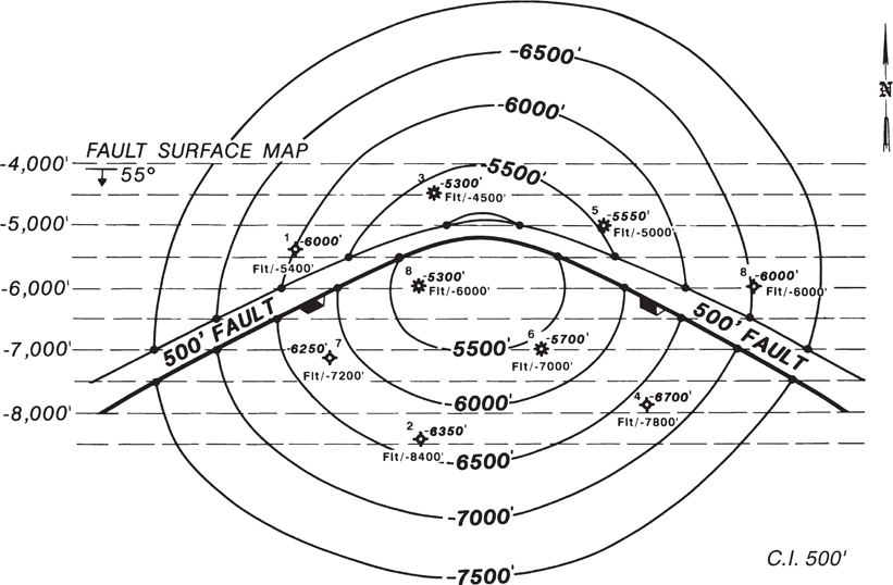
Figure 8-27 A fault surface map superimposed on a completed structure map to show that the fault traces have been determined by the integration of the fault and structure maps. Observe the change in the width of the fault gap across the structure. The change gives the appearance that the fault is smaller near the crest of the structure. (Prepared by J. Bollick. Published by permission of Tenneco Oil Company.)
In Figure 8-10, the curvature of the fault trace and width of the fault gap change across the structure. The gap changes from 350 ft on the flanks to 250 ft near the crest, whereas the fault has a constant vertical separation of 300 ft. Figures 8-11a and 8-12 show a significant difference in the width of the fault gap, which ranges from an average 420 ft in Figure 8-11a to 290 ft in Figure 8-12, despite that the fault on each map is the same fault, with a vertical separation of 400 ft. Finally, examine Figure 8-27, which shows a map of a fault surface, striking east-west and dipping to the south at 55 deg, superimposed on the structure map of the 5500-ft Horizon. The upthrown and downthrown fault traces, and therefore the fault gap, were constructed using the integration technique. Notice how the fault gap thins near the crest of the structure, causing the vertical separation of the fault to appear smaller on the crest than on the flanks. The vertical separation of the fault only appears to change across the structure because the width of the fault gap changes.
The width of a fault gap depends on the amount of vertical separation and the angles and directions of the fault dip and the horizon dip. Therefore, the width of a fault gap for any given fault on a structure map cannot be intuitively determined. It is extremely difficult at best, regardless of vertical separation and our ability to see in three dimensions, to predict the position of fault traces and the width of a fault gap by looking at fault data, or even at a fault surface map and a structure map independently. Examine Figure 8-27 again and ask yourself whether you could have predicted the curvature of the overall fault trace and the variation in width of the fault gap on this final structure map simply by reviewing the fault surface map and structure map data separately without integration. Most likely, your answer is no. We emphasize that if the construction of the upthrown and downthrown fault traces is done properly by integrating the fault and structure maps, the width of the fault gap is automatically constructed without any need for guesses or estimations (Tearpock and Harris 1987).
Rule of 45
Figure 8-28 shows a special condition in which the fault traces can be delineated with reasonable accuracy, without integrating a fault and structure map, and where the fault gap is equal in width to the amount of missing section in the well. The technique used for this situation is known as the rule of 45. If a fault is inclined at 45 deg and the beds are approximately horizontal (zero degree dip), the position of the traces can be identified with reasonable accuracy without integration. The width of the fault gap is equal to the amount of vertical separation for the fault, measured off using the map scale as reference (see map insert in Fig. 8-28).
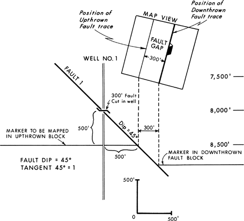
Figure 8-28 The rule of 45. On any given mapped horizon, the horizontal distance from a well to the nearest fault trace is equal to the vertical difference in depth between the fault and the horizon in the well, if the fault is dipping at 45 deg and the mapped horizon is horizontal. In these specific circumstances, the width of the fault gap will be equal to the missing section in the well, which is equal to the vertical separation of the fault.
Consider Figure 8-29a. It is a prospect map illustrating a hydrocarbon trap upthrown to a fault and limited down-dip by a water contact in Well No. 3. The interpretation is based on both well log and seismic data. The completed structure map shows the horizon tops, fault data from the wells, and the subsea depths of the fault at various shotpoints on the seismic lines. The prospect map with a proposed location looks very attractive at first glance.

Figure 8-29 (a) Prospect map based on well log and seismic data. Position of the fault trace based on the rule of 45 relative to the well locations and on the fault position as interpreted on the seismic profiles. (b) Reinterpretation of prospect map in (a), based on integration of the fault surface map with the horizon map. Fault trace moves about 900 ft north. (c) Fault surface map. (Published by permission of D. Tearpock.)
Without detailed knowledge of how the interpretation was generated, management might approve the drilling of such a location. However, upon detailed investigation, it is learned that the completed trace for Fault B was prepared using the position of the fault on the horizon from the two seismic lines and the rule of 45 to position the trace relative to the well locations. Does the application of this method provide a reasonable interpretation in this example? The answer is no. One major structural feature not considered in using the rule of 45 was the structural dip: the horizon is far from flat. As we have shown, bed dip is one of the structural features that affects the position of a fault on a completed structure map.
The structure map shown in Figure 8-29b was prepared using the same structural and fault data. In this case, however, a fault surface map was first constructed (Fig. 8-29c) and then integrated (cross-contoured) with the structure map to arrive at the correct positioning of the upthrown and downthrown fault traces.
The correct integration illustrates that the original prospect map has an enormous error regarding the position of the fault and the prospect potential. This error would result in the proposed well being drilled downthrown to Fault B, missing the oil reservoir entirely. How often can a petroleum company afford such mistakes? A number of prospect maps reviewed worldwide have shown similar mistakes resulting in costly dry holes. And in one particular case, one company drilled two such dry holes in one year. The company’s CEO stated that no additional prospects would be drilled without constructing fault surface maps and integrating the fault with the structural interpretation.
Tangent or Circle Method
Another technique, referred to as the tangent or circle method (Lyle 1951; Bishop 1960), can be used to quickly delineate the approximate position of the fault traces in areas where the beds are nearly horizontal. Lyle introduced this technique in 1951 for mapping faults in southwest Texas and Bishop (1960) diagrammatically illustrated its use.
Figure 8-30a is a base map showing the depth of a normal fault and the depth to the top of a key horizon in each well. More than one fault is represented. The tangent or circle method is used here to quickly prepare a structure map including the fault traces. This technique is good for rapidly checking a completed structure map for accuracy of the positioning of the fault traces. The use of this method requires a low to flat bed dip and knowledge of the dip angle of each fault.
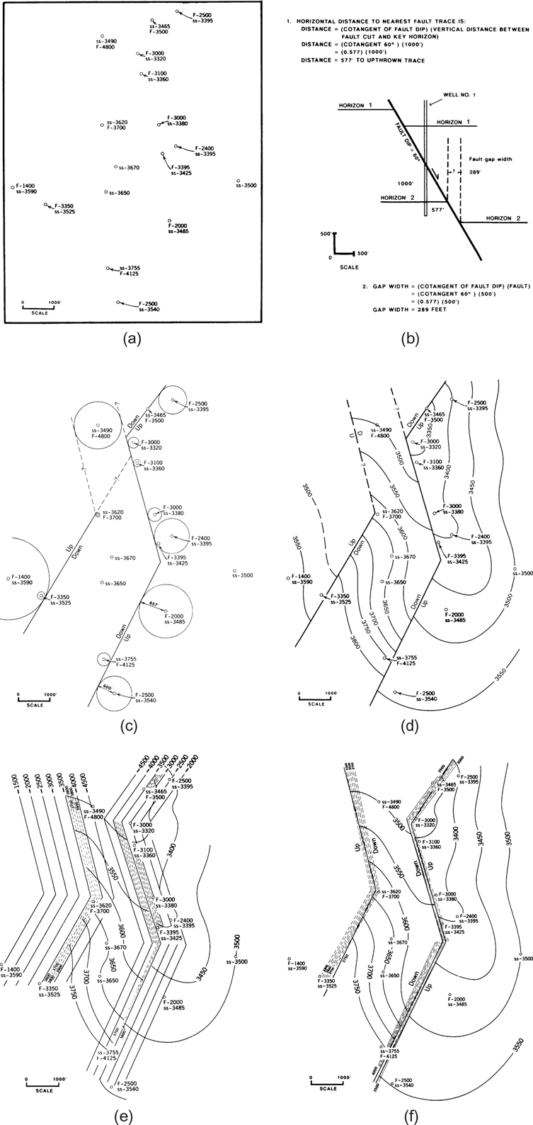
Figure 8-30 (a) Basemap with the depth to fault picks (F−3100 ft) and sand tops (ss -3320 ft) posted. (Modified after Bishop 1960. Published by permission of author.) (b) Determination of the horizontal distance from a well to the nearest fault trace using the cotangent rule and the width of the fault gap. (c) Assumed angle of fault = 60 deg. The position of the fault trace is determined by the circle method. (Modified after Bishop 1960. Published by permission of author.) (d) Structure contour map. Position of the fault determined by the circle method. (e) Integration of mapped horizon and fault surface maps to determine the position and width of the fault gaps. (f) Final integrated structure map. Compare position of fault traces with those shown in Figure 8-30d. (From Bishop 1960. Published by permission of author.)
The horizontal distance between the well and the fault trace on the horizon equals the cotangent of the dip angle of the fault multiplied by the vertical distance between the fault pick and the horizon in the well (Fig. 8-30b).
The well serves as the center point of a circle, the radius of which equals the distance between the fault and the well as determined in step 1 (Fig. 8-30c).
A tangent common to two or more circles determines a fault trace. The exterior tangent is the fault trace for wells on the same side of the fault; the interior tangent is the fault trace for wells on the opposite sides of the fault (Fig. 8-30c). Refer again to Chapter 7, Figure 7-9, and the accompanying text for determining in which fault block a well is located for any mapped horizon.
Finally, contour the horizon tops assuming continuity of structural attitude across the faults (Fig. 8-30d).
If the beds are horizontal, the fault gap width can be determined as shown in Figure 8-30b. Then the fault gap can be drawn on the structure map rather than representing the fault as one line, as shown in Figure 8-30d. This method of estimating the fault trace is useful if the dip of the fault surface can be determined or at least assumed with some degree of certainty and if the horizon being mapped is approximately horizontal. Compare the mapping results in Figure 8-30d with those shown in Figure 8-30e and f. Figure 8-30e is a fault map for the two faults, and Figure 8-30f shows the fault traces constructed by the integration of the fault and structure maps. The position of the fault in Figure 8-30d compares very favorably with the position of the fault in Figure 8-30f, showing that in an area of relatively flat beds, the tangent method can provide a good approximation for positioning the fault on a structure map. However, we caution that this technique does not work in areas of dipping beds.
In Figure 8-30c and d, the fault traces are constructed as straight-line segments with sharp angular changes in strike direction. In order to prepare a more accurate map, the change in strike direction can be smoothed to best fit the overall pattern of the faults and the data in the area being mapped. The fault surface map for Figure 8-30e and the integrated structure map in Figure 8-30f were also constructed as straight-line segments to make the results comparable with those in Figure 8-30d.
The tangent method is not accurate if the horizon being mapped has significant dip (more than 5 deg) because the wellbore is then not perpendicular to the bedding. The correct construction of the fault traces and fault gap for faults on a dipping structure is especially critical because the fault position has a significant impact on any proposed location for an exploration or development well. Figure 8-31a shows a portion of a structure map on the flank of a piercement salt dome. The depth to the mapped horizon and the missing section and depth of the faults are shown next to each well. Since the fault is a perfect plane with a dip of 45°, the structure map in Figure 8-31a was prepared (incorrectly) using the rule of 45 to determine the position of the fault traces and the width of the fault gap. As an example, look at Well No. 6 shown in the figure insert. The fault cuts the well at −9510 ft and the top of the horizon intersects the well at −9395 ft. From the figure insert, we see that Fault A crosses the well 115 ft below the mapped horizon. Therefore, based on the 45-degree trigonometric relationship of 1 to 1, the downthrown trace of the fault was located 115 ft west of the location of Well No. 6, as the horizon in the well is in the downthrown block. Also, since the fault has a dip of 45 deg, the width of the fault gap was scaled to equal the missing section of the fault (400 ft). Using this method, the fault cut in Well No. 3 does not fit as part of the same fault identified in Wells No. 2, 5, 6, and 10; therefore, a second fault, Fault B, was postulated as shown on the figure, resulting in an untested fault trap up-dip of Well No. 5.
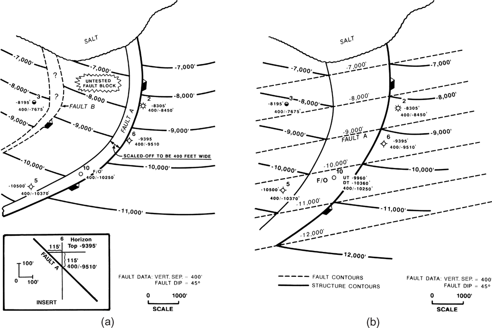
Figure 8-31 (a) Portion of a structure map on a steeply dipping horizon on the flank of a piercement salt dome. The map was incorrectly prepared using the rule of 45 to position the fault traces. Although the fault is dipping at 45 deg, the rule of 45 is not applicable because the beds are not horizontal. (b) Correctly contoured structure map based on the integration of the structural interpretation with the fault surface map. Compare this map to that shown in Figure 8-30a.
The fault in this example has a constant dip of 45 deg and, in this respect, the above methods were appropriate. However, the beds are not horizontal; they dip quite steeply (about 40 deg in the up-structure position). Therefore, neither the rule of 45 nor the tangent method is appropriate for the preparation of the structure contour map in Figure 8-31a. Figure 8-31b shows the fault surface map and the correctly contoured structure map for this horizon. The fault is a peripheral fault paralleling the face of the salt; the beds are dipping at about 40 deg at −7000 ft and flatten to about 32 deg between −11,000 ft and −12,000 ft. Since the beds are steeply dipping, the fault map was required for integration of the fault and structure maps to delineate accurately the fault traces on the structure map. The upthrown and downthrown traces of the fault, and therefore the resulting fault gap, were constructed using the integration technique discussed earlier in the chapter.
Observe that although the fault has a constant vertical separation of 400 ft (as determined from well log correlation), and the fault is a perfect plane dipping at 45 deg, the trace of the fault is curved and nowhere along its trace is the gap 400 ft wide. Measuring across the fault gap at the location where the −8000-ft structure contour in the upthrown block intersects the upthrown trace of the fault, the width of the fault gap is approximately 1700 ft. At the intersection of the −10,000-ft structure contour and the upthrown trace of the fault, the width of the fault gap has decreased to 1200 ft. If a well were drilled, on the basis of the map in Figure 8-31a, in the “untested fault block,” then the mapped horizon would probably be faulted out of that well (as shown by the correct map in Figure 8-31b). Study this figure very carefully, for it shows how important it is to integrate the fault and structure maps on steeply dipping structures to accurately position the fault traces and delineate the fault gap.
As a general rule of thumb, we consider any structure with a dip greater than 5 deg as steeply dipping for purposes of fault and structure map integration. However, to prepare a structure map as accurately as possible regardless of the structural dip, the integration technique should always be used to delineate the position of the fault traces and the width of the fault gap.
Figure 8-32 shows three different sets of integrated fault and structure contour maps that result in significantly different fault traces and gaps. For example, the set on the left side of the figure consists of completed structure maps A(1), B(1), and C(1), all of which use the same oblique down-dip fault with 100 ft of vertical separation to integrate with the structure. A(1) shows a horizon with a dip that is constant, B(1) shows a steeply dipping horizon which increases in dip in the upstructure direction, and C(1) is similar to B(1) except that the horizon dip is less. Despite the constant fault surface in all three cases, each integrated structure map results in a strikingly different fault trace pattern and fault gap width. Take a few minutes to review the different fault traces and gaps for sets 2 and 3 in Figure 8-32.
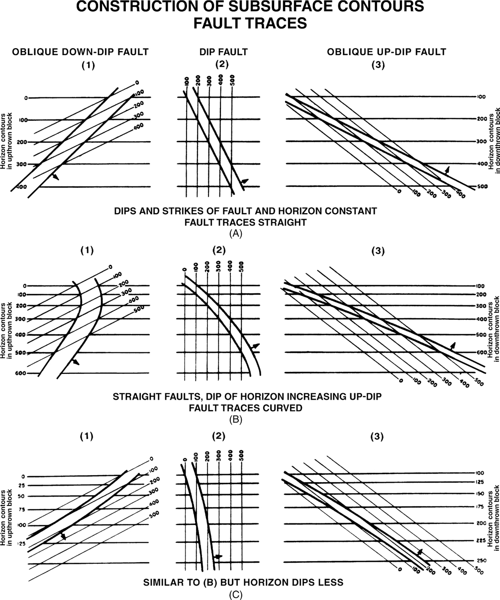
Figure 8-32 Three different sets of integrated fault and structure maps illustrating significantly different fault traces. (Published by permission of Tenneco Oil Company.)
The nine separate patterns shown in Figure 8-32 and those in Figures 8-10, 8-26, 8-27, and 8-31 reinforce our statements that the final fault traces and fault gap for any particular set of fault and structural conditions are not intuitively predictable and, in fact, are often impossible to predict without actually integrating the two surfaces. The precise positioning of the fault traces and delineation of the width of the gap or overlap (in the case of a reverse fault) can mean the difference between generating and not generating a prospect, the difference between drilling a successful well versus a dry hole, or the difference between a reservoir whose calculated volume matches its performance versus a reservoir that appears to either have overproduced or underproduced the volumetric estimate of reserves. Taking shortcuts to identify the positions of fault traces and to determine the widths of fault gaps is a risky business unless the beds are relatively flat-lying and the fault dips are very close to 45 deg.
New Circle Method
We have emphasized the importance of integrating a fault and structure map in areas of dipping beds to accurately delineate a fault trace. We have also developed a mathematical relationship that can be used in areas of dipping beds to estimate the approximate position of the fault traces, if there is sufficient well control. These equations can be used as a quick check when reviewing structure maps.
Two equations are required for this method. The first equation estimates the distance from a well (radius of a circle) to the nearest fault trace, and the second estimates the heave of the fault, which is used to locate the position of the other trace of the same fault. The strike direction of the fault must be known in order to determine the direction in which to measure heave. The equations are shown here and illustrated in Figures 8-33 and 8-34.
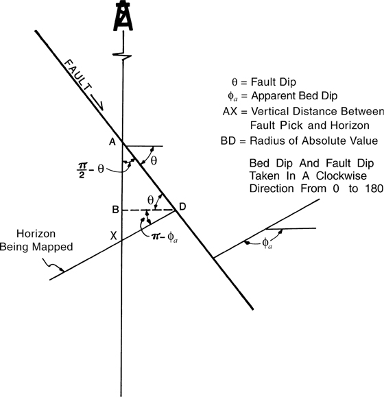
Figure 8-33 Diagrammatic illustration of the fault and formation parameters used to derive Eq. (8-2). View is perpendicular to strike of fault surface.
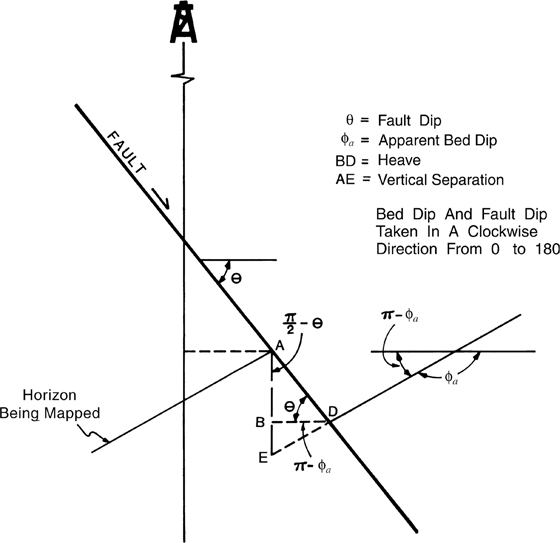
Figure 8-34 Diagrammatic illustration of the fault and formation parameters used to derive Eq. (8-3). View is perpendicular to strike of fault surface.
Equation to Determine Radius of Circle
From the law of sines and Figure 8-33,
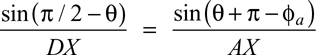
and
Therefore,
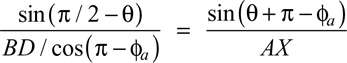
or
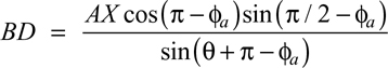
Therefore,
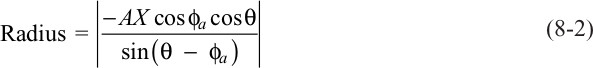
where
If ϕa = π, then Eq. (8-2) becomes
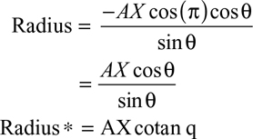
Equation to Determine Heave
Utilizing the law of sines and Figure 8-34,
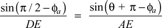
and
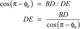
Therefore,

which is the same form as the radius Eq. (8-2). For example,
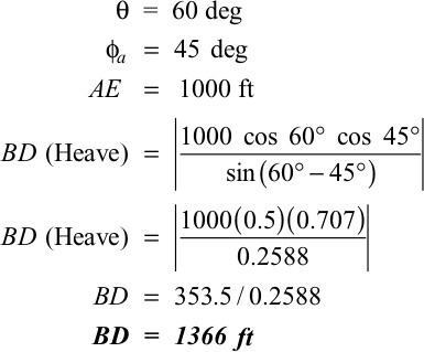
In order to use these equations, the strike direction of the fault surface must be known. These equations should be used only as a quick look or check; they do not take the place of the fault/structure integration technique.
Fault Gap Versus Fault Heave
Before leaving the subject of fault gap, we briefly discuss the fault component heave, which is often misused or mistaken for fault gap. Fault gap is the horizontal distance between the upthrown trace and downthrown trace of a fault measured perpendicular to the strike of the fault traces. Fault heave is the horizontal distance between the upthrown and downthrown traces of a fault measured perpendicular to the strike of the fault surface itself. The width of a fault gap is equal to fault heave only where the beds are horizontal, or nearly so, and the strike of the fault is parallel to the strike of the formation. Considering most other situations, the width of the fault gap and the fault heave are not the same. Therefore, the term fault gap (or overlap in the case of a reverse fault) is not synonymous with fault heave.
The completed structure map in Figure 8-31b clearly illustrates the difference between fault gap and fault heave. Using the completed structure map, measure the heave for Fault A at the location where the −9000-ft contour in the upthrown block intersects the upthrown trace of the fault. First, draw a reference line perpendicular to the strike of the fault surface at the intersection of the −9000-ft structure contour with the −9000-ft fault contour. This line intersects the downthrown trace of the fault at some point. Using the horizontal reference scale on the map, measure the length of this reference line, which is the measurement of fault heave at this location along the fault. The fault heave is equal to about 1825 ft. Now the distance across the gap at the same −9000-ft point, measured perpendicular to the upthrown trace, is equal to 1425 ft. Therefore, we can see that the heave is not equal to gap and they are measured in two completely different directions.
Now, take a minute to determine the throw of the fault, using the same reference line. If done correctly, the line intersects the downthrown trace of the fault at a depth of about −10,825 ft so the fault throw is 1825 ft (10,825 ft − 9000 ft = 1825 ft). Since the fault has a dip of 45 deg, the throw of the fault must equal the heave, or 1825 ft. We can easily check the measured result for fault throw by using Eq. (7-1). To use the equation, the bed dip must be averaged for the interval between the −9000-ft contour in the upthrown block to the −10,825-ft contour in the downthrown block because the gap is too wide and bed dip changes rapidly in this area. For the equation, use 38 deg as an average bed dip. Also, use Eq. (8-3) to estimate the fault heave mathematically and compare the results with the measurement shown in Figure 8-34.
These measurements are shown in Figure 8-35. Notice for this example that there is a significant difference between the strike direction of the fault gap and that for the fault heave. Fault heave and fault gap are different fault components that cannot be referred to interchangeably. As another exercise, measure the fault overlap and heave at some point on the reverse fault shown in Figure 8-26b and compare the results.
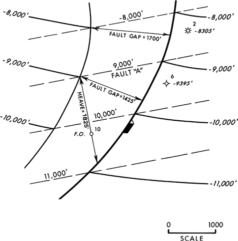
Figure 8-35 A part of Figure 8-31b illustrating the measurements of fault gap and fault heave.
Subsurface geoscientists should, as a general rule, avoid using the terms throw and heave and should always refer to measurements derived from log correlations and map construction as vertical separation and fault gap width (Tearpock and Harris 1987).
Structure Map—Generic Case Study
In the section Techniques for Contouring across Normal Faults, we present the technique for projecting established contours from one fault block across a fault into the opposing fault block to contour correctly the displacement resulting from a fault. The displacement to which we refer is vertical separation, as determined from well log correlations or seismic data. In the same section, the incorrect technique of contouring displacement as throw is also presented. Now we look at a generic case study that illustrates the impact of preparing a map with the incorrect, as opposed to correct, contouring technique.
This field example shows an anticline cut by a large 600-ft down-to-the-south normal Fault A and a smaller 100-ft antithetic (compensating) normal Fault B (Fig. 8-36). The structure map in Figure 8-37a was prepared with the incorrect assumption that the missing section in the wellbores is equal to throw (note the dashed contours in the fault gap drawn perpendicular to the strike of the fault). Based on this interpretation, two development wells are proposed. Location X, upthrown to Fault A in Reservoir A, is estimated to penetrate the reservoir up-dip and to the east of Well No. 12 at a depth of −4960 ft. The purpose of the well is to improve the drainage efficiency of this reservoir. Location Y, upthrown to Fault B, is estimated to penetrate Reservoir B at a depth of −5360 ft and is designed to be drilled in the optimum structural position to drain the attic reserves in this reservoir.
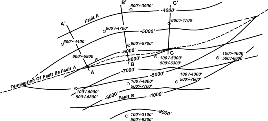
Figure 8-36 Fault surface map (Faults A and B) for the generic case study. (Published by permission of Tenneco Oil Company.)
The structure map in Figure 8-37b was constructed correctly, using the missing section in the wellbores as vertical separation. Observe the dashed contours in the fault gap showing the trend projection of the contours from one fault block to the next. This correct interpretation shows a different structural picture. First, Well X is estimated to penetrate the formation at a subsea depth of −5030 ft, which is the depth of the oil/water contact in Reservoir A. Therefore, Well X, if drilled, would probably be a dry hole. The penetration point for Well Y, in Reservoir B, is estimated at −5415 ft, or 55 ft deeper than that shown in Figure 8-37a. Based on the correctly contoured map, the proposed well is about 800 ft west of the optimum position to efficiently drain the remaining reserves in Reservoir B.
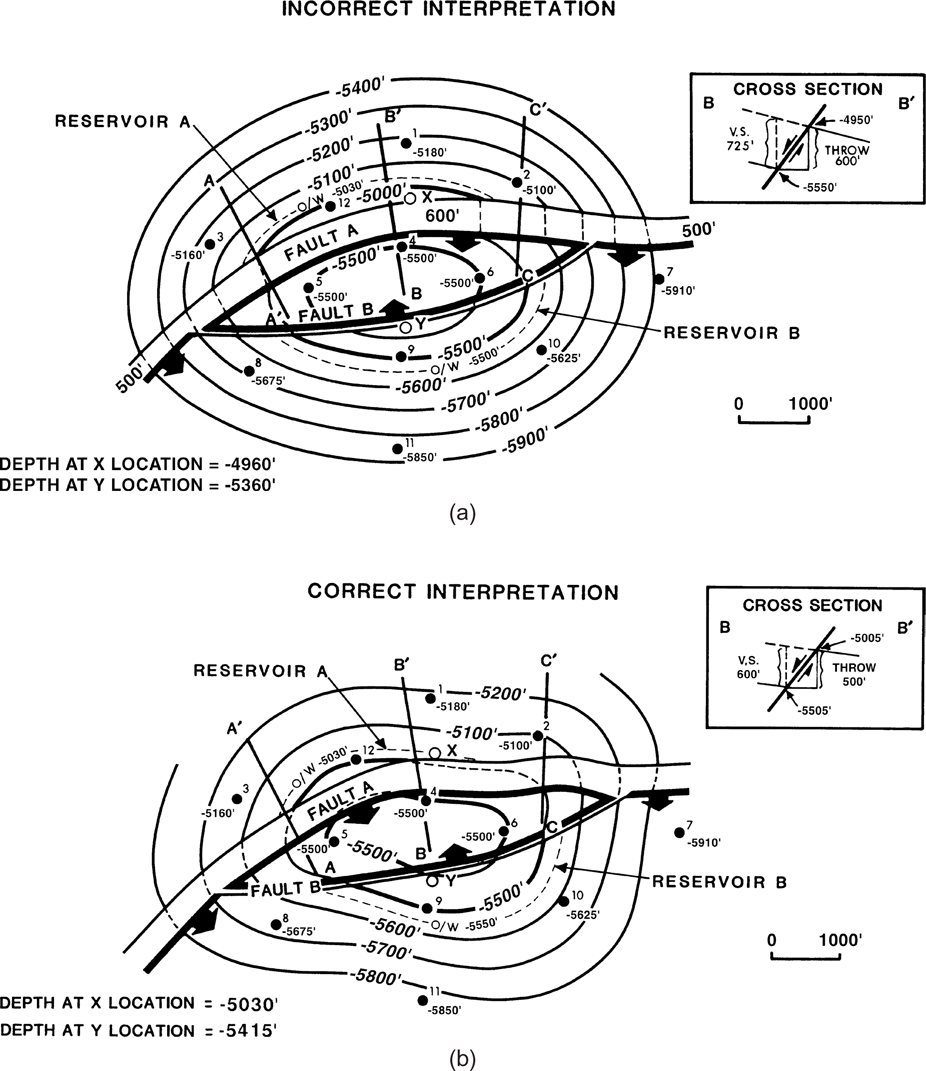
Figure 8-37 (a) Generic case study: structure map prepared using missing section (vertical separation) incorrectly as if it were throw. (b) Generic case study: structure map prepared using vertical separation to correctly contour across Faults A and B. (Published by permission of Tenneco Oil Company.)
The correctly contoured map has the following impact on these two reservoirs and proposed wells.
Reservoir A (upthrown to Fault A)
It eliminates the drilling of a dry hole.
It improves the volumetric reserve estimate, in this case, a 36% reduction in reserves.
Reservoir B (upthrown to Fault B)
It improves the volumetric reserves estimate for the reservoir (a reduction of 11%).
It improves the configuration of the reservoir, affecting the location of the proposed development well.
The magnitude of error created by incorrectly mapping vertical separation as if it were throw is greatest near or on the crest of a structure, as illustrated in this generic case. On both the east and west flanks of the structure, where the strike direction of the contours is nearly perpendicular to the strike of the fault, the projection of contours through the fault is almost identical for both structure map interpretations. Where the strike direction of the structure contours is perpendicular to the strike of the fault, lines parallel to the structure contour strike, or a cross section in this orientation, give the appearance that the formation has an apparent dip of zero degrees (horizontal). Therefore, whether the contours are projected through the fault as if the fault were not there (mapping vertical separation), or the strike direction of the contours is projected through the fault perpendicular to the strike of the fault (mapping throw), the direction of contour projection through the fault is similar. However, as the crest of the structure is approached, the projection of the contours is radically different for each structure map. Review the −5000-ft contour starting in the upthrown block of Fault A and follow the projection across the fault into the downthrown fault block on both maps; notice the significant difference in contour projections. Here again we emphasize that it is very important to contour correctly over the entire map, but it is especially critical in and around the crest of a structure where hydrocarbon accumulations are expected to occur.
Three cross-section lines are shown on each structure map. The B-B′ cross section for each map is shown in the upper right corner of Figure 8-37a and b. The B-B′ section in Figure 8-36a shows that if the throw of the fault were 600 ft as mapped, then the vertical separation in cross section B-B′ would have to be 725 ft; therefore, the missing section in the wells would also have to be 725 ft. The B-B′ cross section in Figure 8-37b shows a vertical separation of 600 ft, which agrees with the missing section in each well and a throw across the fault at this location of 500 ft. This cross-section geometry is supported by the well log data and the completed structure map. As a cross-section exercise, complete sections A-A′ and C-C′ for both maps and evaluate the results. If you are interested, use Eq. (7-1) again to test the validity of the structure contour map in Figure 8-37b.
The Additive Property of Faults
In the preparation of accurate structure maps, the vertical separations of intersecting faults will balance across the intersection. This is sometimes called the additive property of the vertical separations. For example, where two faults merge into one, the vertical separation of the “surviving” fault is equal to the sum of the vertical separations of the two merging faults. This property is referred to by several names, including the additive property of faults, conservation of vertical separation, conservation of fault size, and (mistakenly) conservation of fault throw.
The additive property of faults, simply defined, states that in areas where two or more faults have an intersecting relationship, vertical separation must be conserved at the intersection. To create a simple calculation to evaluate that, we say that the algebraic sum of the vertical separations must equal zero around the intersection of the faults. Figure 8-38a, which is a structure map of a bifurcating fault system, is used to demonstrate the calculation. First, imagine a circle around the fault intersection. Then proceed clockwise around the intersection and note the vertical separations as determined from contours, or interpolated contours, close to the intersection. Assign a positive value to the vertical separation if the clockwise path across the fault is from the upthrown to the downthrown block. Conversely, assign a negative value if the path across the fault is from the downthrown to the upthrown block. Beginning at the 12 o’clock position, the first fault encountered has a vertical separation value of +400 ft (−7800 ft versus −7400 ft). The next fault has a vertical separation value of −150 ft, using an interpolated contour of −7550 ft versus the downthrown contour of −7700 ft. The third fault has a vertical separation of −250 ft. The sum of the three values is zero.

Figure 8-38 Conservation of vertical separation at fault intersections. (Published by permission of Tearpock et al. 1994.)
Simplified maps of fault patterns in Figure 8-38b and c further illustrate the method. Using the compensating pattern in Figure 8-38b and beginning at the 12 o’clock position, the first fault encountered has a vertical separation of +1200 ft. The second fault has a −400-ft vertical separation, and the third fault has a vertical separation of −800 ft. So the algebraic sum equals zero. An intersecting fault pattern is shown in Figure 8-38c. Proceeding from the 12 o’clock position, we cross four faults that have successive vertical separation values of −200 ft, +300 ft, +200 ft, and −300 ft. Again, the algebraic sum equals zero.
This additive property is very important to keep in mind when preparing structure maps involving intersecting faults, and the property is also quite helpful in quickly evaluating or reviewing completed structure maps. A failure in the test of the additive property of faults can indicate a structure mapping problem. Often it is easy to identify the mapping bust, but difficult to determine why there is a problem. Sometimes the problem is the result of incorrect contouring, a misunderstanding of the property, or a well log or seismic correlation bust.
The example shown in Figure 8-39a is probably the result of incorrect contouring and failure to integrate the fault and structure maps. This completed map shows an intersecting compensating fault pattern with Fault A dipping to the north and having a vertical separation of 400 ft at the intersection (−12,400 ft versus −12,000 ft) and Fault B dipping to the southwest and intersecting Fault A. Fault B becomes smaller to the south so that near the intersection, the vertical separation is only 100 ft. Therefore, the vertical separation of the resultant Fault A east of the intersection must be 300 ft (400 ft −100 ft = 300 ft); however, it is contoured as 450 ft on the map.
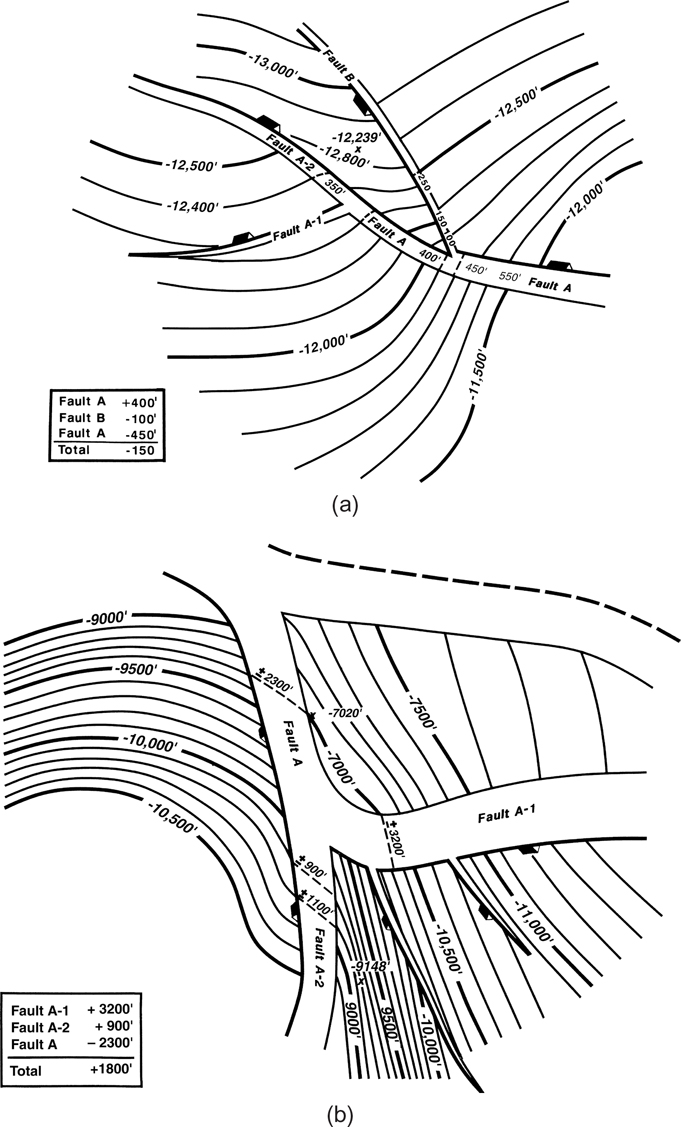
Figure 8-39 (a) Vertical separation is not conserved around the intersection of Faults A and B. This mapping bust appears to be the result of incorrect contouring and the failure to integrate the fault and structure maps. (b) The failure to conserve the vertical separation around the intersection of Faults A-1 and A-2 in this example is significant. This mapping bust is probably due to a seismic correlation mis-tie across one or both of the intersecting faults. (Modified from Tearpock and Harris 1987. Published by permission of Tenneco Oil Company.)
There appear to be three separate problems with this structure map. (1) Although this is a compensating fault pattern, the map is prepared incorrectly, depicting a bifurcating pattern where the individual vertical separations for Faults A and B are added. The 400 ft for Fault A added to the 100 ft for Fault B equal 500 ft. Notice that the vertical separations do not even add correctly, which is another problem related to the completed map. (2) It is obvious that this map was prepared without being integrated with fault maps. When fault and structure maps are integrated, the fault traces and gaps are properly constructed. Thus, an error of constructing fault traces that depict the addition of fault vertical separation rather than their subtraction, such as in the case of this compensating fault pattern, would not occur. (3) The contouring across Fault A is incorrect at the intersection. The contours on opposite sides of Fault A east of the intersection should have an elevation difference of 350 ft rather than the 450 ft contoured on the map, since this is a compensating fault pattern.
Using tracing paper, recontour this map (Fig. 8-39a) to reflect an acceptable structural interpretation around the fault intersection. Finally, examine the structure map further for mapping busts in contouring across Fault A-2 and the intersection of Fault A-2 with A-1. See if you can identify and correct these problems.
Figure 8-39b shows another example of a completed structure map, generated from seismic data, that fails to honor the conservation of vertical separation. Unlike the cited error in Figure 8-39a, which is minor as errors go, the error in Figure 8-39b is quite significant. A test of the additive property of faults around the intersection of Faults A, A-1, and A-2 indicates an error on the order of 1800 ft. Such a significant error is not due to incorrect contouring, but is most likely the result of a seismic correlation mis-tie across one or more of the intersecting faults. Look at the structural dip direction for the westernmost fault block versus the fault block upthrown to Faults A and A-1. What are your thoughts?
Integration of Seismic and Well Data for Structure Mapping
In Chapters 5 and 7 we cover the basic techniques for integration of fault data determined from seismic sections. In this section, we discuss the additional data provided by seismic sections to assist in the construction of subsurface structure maps. The lateral resolution of seismic data contributes information away from well control and helps define a larger, more continuous surface than is mappable from well data alone.
This discussion assumes that several conditions have been met before the seismic data are used to make a structure map. The first condition is that the seismic data have been correctly processed. The second condition is that the seismic lines have been approximately tied into the event that is correlative with the actual horizon being mapped. In some areas this may be simply a matter of using the correct velocity function to locate the proper time event that corresponds to the horizon. In more complex areas, the tie to seismic information may require the use of a synthetic seismogram or vertical seismic profile to locate the proper event to map.
The third condition is that there should be no significant velocity changes over the area being mapped. If a lateral velocity gradient appears to be present, a gradient map may be required to deal with this problem. If the seismically derived horizons do not agree with the horizons in the wells across the area being mapped, there are several potential reasons for this disagreement. First, a velocity gradient may be present. These are common in some areas and rare in others. Second, the well log or seismic correlations may be wrong. Look hard at both sets of data before modifying or discarding one of them. Third, the wrong event may be interpreted as corresponding to the horizon being mapped. This can cause problems, especially in areas of extreme thinning and thickening of the stratigraphic intervals.
If the velocity field is uniform over the area, or if appropriate adjustments have been made for a nonuniform velocity field, then seismic data can be extremely valuable in subsurface structure mapping. Seismic data provides (1) estimates of structural elevations for the horizon being mapped; (2) continuous dip information along the seismic line; and (3) accurate structural data points at the intersection of faults with the horizon along the seismic line. The use of a 3D data set allows the geoscientist to actually interpret and map a 3D data volume.
Figure 8-40 shows an example of seismically derived data that can be posted to aid in the construction of a subsurface structure map. The first and most obvious data points are the horizon depths posted at the shotpoint locations. These values are seismic time picks converted to depth with the appropriate velocity function. Second, fault data are posted along the intersection of the faults with the horizon. For example, line D illustrates how to post the upthrown and downthrown elevations for the mapping horizon at the intersection of the horizon with the fault along the line of section. For Fault B, the upthrown elevation of the intersection of the horizon with the fault is −9460 ft, and the downthrown elevation at the fault/horizon intersection is −9815 ft. Finally, the vertical separation data estimated across the fault are posted and used to aid in the mapping (e.g., 450 ft for Fault B on Line D).

Figure 8-40 Completed structure map illustrating seismically derived subsurface data used to prepare the map. Depths are in feet. (Prepared by C. Harmon. Modified from Tearpock and Harris 1987. Published by permission of Tenneco Oil Company.)
When using seismic data, be aware of the difference between the apparent throw values and the vertical separation, and label the latter on the map. The estimate for apparent throw is the difference in elevation between the upthrown and downthrown intersections of a horizon with the fault along the line of section. Notice the changing values for apparent throw along fault A; these changing values are a function of the orientation of the line of section crossing the fault (lines B, D, and E). However, the values for the vertical separation along this portion of the fault do not change. For example, based on the upthrown and downthrown values measured along lines E, B, and D, the apparent throw of Fault A is 520 ft at line E, 425 ft at line B, and 375 ft across line D. Considering these apparent throw values, the fault could be incorrectly interpreted as decreasing in size or dying to the east. But the estimate of the vertical separation at each line shows that vertical separation for Fault A is a constant 500 ft in the area east of the intersection with Fault B. Contrast this with Fault B, which shows a decreasing vertical separation as the fault dies laterally to the east; however, the apparent throw, as measured from line D, is 355 ft, and it is 325 ft from line B, suggesting a fault of almost constant apparent throw. It is most common to use the vertical separations for mapping displacement across faults, whether the data are from well logs or seismic sections.
The contouring techniques presented at the beginning of this chapter apply to the use of seismically derived data as well as log data. Seismic data offer some additional advantages that are lacking in well data, such as the ability to post upthrown and downthrown mapping control points at fault/horizon intersections. These additional data give two more control points to help in contouring the final structure map.
In summary, seismic data allow us to extend the interpretation beyond the limits of well control. It helps in the construction of a continuous subsurface picture of the horizon being mapped and provides additional, more complete information about the characteristics of the faults that intersect these horizons.
Other Mapping Techniques
Mapping Unconformities
An unconformity is a surface of erosion and/or nondeposition that separates strata of different ages. The development of an unconformity involves several stages of activity. The first is the deposition of the initial sediments; second, the area is subject to uplift and subaerial erosion and/or nondeposition, developing an unconformable surface; and third, the deposition of younger sediments above the unconformity. Unconformities are present in all geological settings, but are especially common on steeply dipping structures.
Unconformities alone, or in combination with faults or stratigraphic anomalies, such as sand pinchouts, serve as locations of excellent hydrocarbon traps (Fig. 8-41). It is therefore important to recognize and map unconformities in the subsurface. In Chapter 4, we present the guidelines to recognizing unconformities by log correlation and dipmeters, and to distinguishing faults from unconformities. In this section we discuss general techniques for mapping an unconformity in the subsurface and integrating that unconformity map with a structure map.
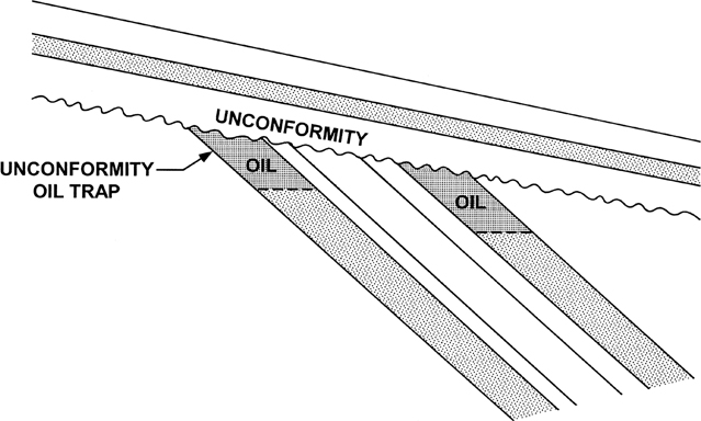
Figure 8-41 Typical hydrocarbon trap beneath an angular unconformity.
An unconformity map is a type of surface contour map. It differs from a typical structure map in that the contours are on an unconformable surface rather than some stratigraphic marker or horizon. Unconformity maps are not normally made to stand alone; instead, they are integrated with a structural horizon map to delineate the intersection of the unconformity with the horizon being mapped. This intersection marks the termination of the horizon at the unconformity. If a hydrocarbon trap is present beneath the unconformity, the termination of the reservoir against the unconformity defines a boundary of the reservoir (Fig. 8-41).
Although there are various kinds of unconformities, for petroleum exploration and exploitation we are primarily interested in two types: (1) angular unconformity and (2) disconformity. An angular unconformity is one in which the rocks above and below the unconformity are not parallel with one another, with the rocks below the unconformable surface typically dipping at a steeper angle than those above. Figure 8-42a is a north-south electric log cross section showing a good example of an angular unconformity determined by log correlation (Lock and Voorhies 1988). Good, easily traceable resistivity markers in the section below the unconformity are seen to be progressively cut out at the unconformity surface. Notice, in the interval above the unconformity, that by correlating down the logs, the section is seen to be interrupted in each well at the same stratigraphic marker. From the Tribal Oil No. 1 to the Sinclair No. 5, as much as 150 ft of section is missing as a result of the unconformity. Angular unconformities and disconformities can often be mapped accurately on seismic data (Fig. 8-42b)
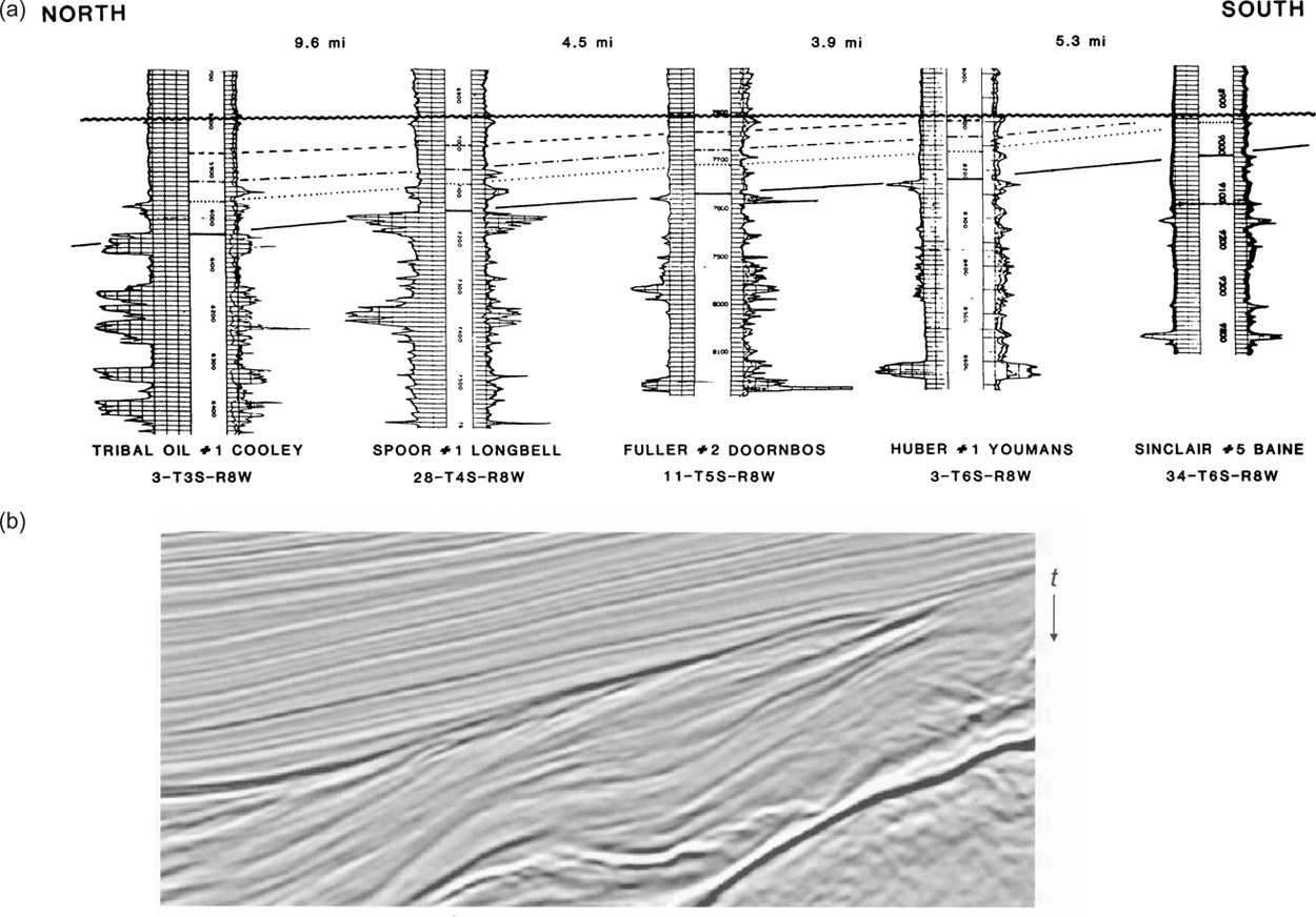
Figure 8-42 (a) Example of an angular unconformity recognized by electric log correlation. (From Lock and Voorhies 1988. Published by permission of the Gulf Coast Association of Geological Societies.) (b) Example of an angular unconformity recognized on seismic data (From Herron 2011. Published with permission from Society of Economic Geophysicists, seismic courtesy of PGS.)
A disconformity is an unconformity in which the rocks above and below the unconformity are approximately parallel. In the subsurface, disconformities are particularly difficult to recognize. In some cases, paleontological data may be helpful, in the absence of evidence based on well log correlation or seismic data.
Unconformities occur on a variety of scales ranging from very local in extent, such as those associated with meandering stream channels across a flood plain, to those covering many square miles. A major unconformity in the area around the western flank of the Sabine Uplift (located along the Louisiana-Texas border in the United States) serves as the trap for the giant (5-billion-barrel) East Texas Oil Field (Fig. 8-43). Actually, this giant field results from the intersection of two unconformities creating the up-dip oil trap in the Woodbine Sandstones. Unconformities are very common around steeply dipping structures, especially salt domes. An excellent example of a major angular unconformity associated with a salt dome is shown in Figure 4-45.
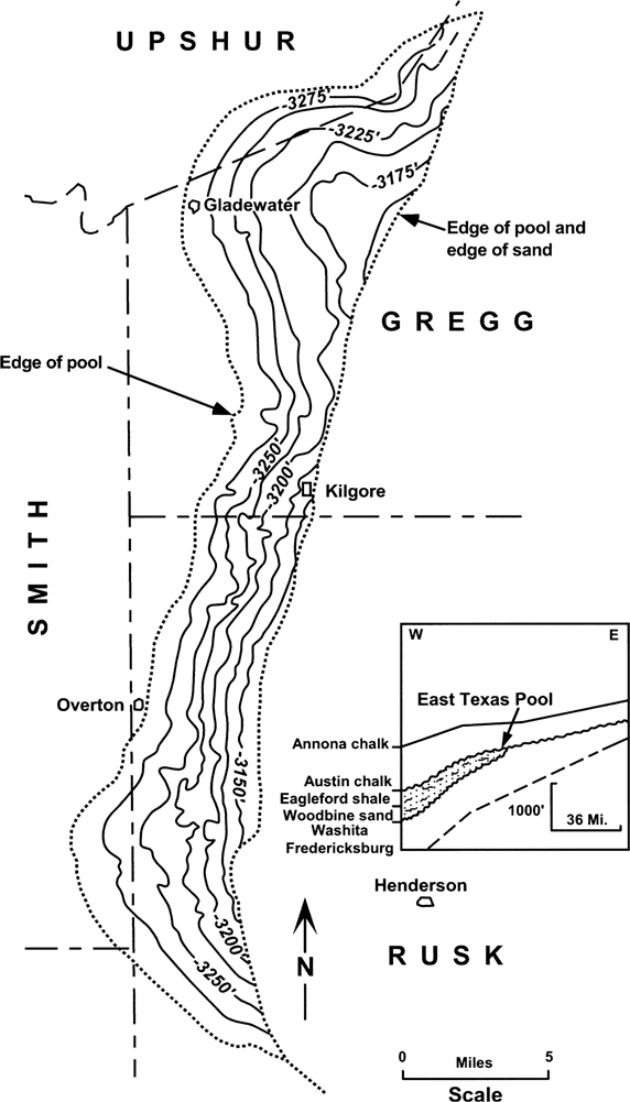
Figure 8-43 Structure map on top of the Woodbine Sand in the East Texas pool. As shown in the cross-section insert, the intersection of two unconformity surfaces marks the eastern boundary of this unconformity trap. (From Geology of Petroleum, first ed. By A. I. Levorsen, Copyright 1954 by W. H. Freeman and Company. Reprinted by permission.)
Mapping Techniques.
Figure 8-44a is a map of a deformed unconformity surface based on log correlations and seismic data. Figure 8-44b shows the integration of the top of Stratigraphic Unit A, which is oil-bearing, with the unconformity, thus delineating the western limit of the horizon against the unconformity. The termination of the mapped horizon against the unconformity is determined by overlaying the structure map on the top of Unit A onto the unconformity map. The intersection of each structure contour for the top of the unit with each unconformity contour at the same elevation delineates the position of the unconformity on the top of Unit A (Fig. 8-44b). This integration is basically the same as that for fault and structure maps.

Figure 8-44 Construction of a map of the top of a reservoir trapped beneath an unconformity. (a) Contour map on an unconformity surface based on both electric log and seismic correlation data. (b) The termination of the top of Unit A is defined by the intersection of the unconformity with the top of Unit A. (c) The intersection of the base of Unit A with the unconformity surface defines the western limit of this oil reservoir Unit A. (d) Map of the top of the reservoir. An unconformity wedge zone is defined as the area between the unconformity traces on the top and base of the sand unit. The map of the wedge zone is a copy of the map of the unconformity in that area. The maps of the wedge zone and the top of Unit A are combined to form the top of reservoir map.
Depending on the scale of the map, thickness of the stratigraphic unit, dip of the beds, and other considerations, a map on the top of a particular stratigraphic unit may not be sufficient to accurately show the effect of the unconformity on that unit. At times, a structure map on the base of the stratigraphic unit is required in addition to a map showing the unconformity wedge between the top and base of the unit. Figure 8-44c is a structure map on the base of Unit A, and it delineates the position of the intersection of the unconformity with the mapped horizon. The procedure for determining the position of the unconformity on the base of the Unit A is the same as that just shown for the top of the unit.
Notice that the unconformity traces on the top and base of Unit A are not in the same position, indicating that there is an unconformity wedge zone between the two traces. This wedge zone can be mapped in combination with the structure map on the top of Unit A in order to depict the top of the reservoir, as shown in Figure 8-44d. This map is prepared by first overlaying the structure map on the top of the unit onto the structure map on the base of the unit and transferring the trace of the unconformity on the base to the structure map on the top of the unit. There are now two unconformity traces on the top of structure map and they delineate the wedge zone. Between these two traces, the reservoir varies from full thickness to zero thickness. Since the structure in the wedge zone is actually that of the unconformity itself, next overlay the top of the structure map onto the unconformity map and trace the structure contours in the wedge zone from the unconformity map. For example, the −6200-ft contour on the top of Unit A, at the trace of the unconformity, continues as the −6200-ft contour on the unconformity in the wedge zone until it intersects the western limit of the wedge zone. Notice that the contour changes strike direction in the wedge. This procedure is followed for all the contours on the map. The result is a structure map on the top of the reservoir. Observe that the unconformity wedge zone for this interval comprises a significant area of the oil reservoir; therefore, in such situations the wedge zone must be contoured.
Mapping across Vertical Faults
High angle and vertical faults, particularly those with small displacements relative to the overall structure, tend to offset the structure without much if any change in the structural attitude across the fault. For a vertical fault, the vertical separation equals throw. Figure 8-45 shows that the throw is 400 ft and the vertical separation is also 400 ft. They are the same because there is no projection of bed dip across a fault gap or overlap. Therefore, we need only concern ourselves with one value for fault displacement when contouring across a vertical fault. For many cases, there is continuity of structural attitude, so the strike direction of the contours is maintained when mapping across the fault. In very complexly faulted areas, however, the strike direction of the contours may be affected from fault block to fault block, particularly if any rotation of the fault block or horizontal displacement occurs.

Figure 8-45 Cross section shows that the values for both vertical separation and throw are the same across a vertical fault.
Figure 8-46 depicts a structure cut by two vertical faults. The contours from one block are projected across the fault into the next fault block. The contours are projected across the fault as if the fault were not there, representing a continuity of structure across the fault, although each contour is adjusted for the vertical separation. This technique assumes no horizontal displacement. Since the fault is vertical, there is no fault gap or overlap, so the fault is depicted as a single line on the finished structure map.
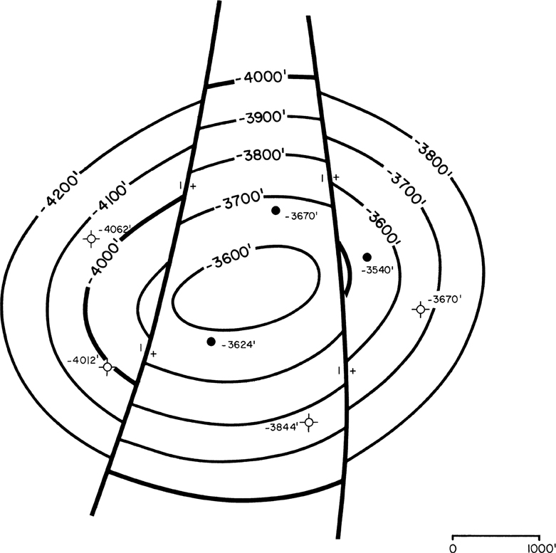
Figure 8-46 Completed structure contour map on the 3600-ft Horizon cut by two vertical faults. The structure contours are drawn from one fault block to the next assuming structural continuity across the faults.
One of the biggest problems with a vertical fault, besides recognizing the presence of the fault, is estimating the vertical separation of the fault for contouring. The fault cannot be intersected by a vertical well. An estimate of the vertical separation must come from intersections of the fault with deviated wells, from seismic data, or from sufficient well control within each fault block to contour both the upthrown and downthrown blocks separately and use the offset contours to determine the vertical separation for the fault.
Top of Structure Versus Top of Porosity
Subsurface structure maps are made on specific stratigraphic units to depict the 3D geometric shape of the geological structures being mapped. Once the geometry of the structure has been determined, the primary effort is focused on the mapping of all hydrocarbon-bearing stratigraphic units.
At times, for various reasons, a structure map is prepared on a good seismic event or resistivity marker that is correlatable in all or most of the wells in a region or field, instead of mapping an actual hydrocarbon-bearing unit. In some cases this may be done because the hydrocarbon-bearing unit is discontinuous or has great vertical variation not reflecting the true shape of the structure. Therefore, it is necessary to prepare a structure contour map first on a stratigraphically equivalent marker in order to construct a map that conforms to the true structure of the field or region. This marker may be a few feet or several hundred feet above the actual hydrocarbon-bearing unit(s). Once the structural framework is prepared by contouring the data from the stratigraphically equivalent marker, a second map, called a top-of-porosity map, is required on the top of any productive unit for the purpose of delineating the actual configuration and limits of the reservoir (Fig. 8-47).
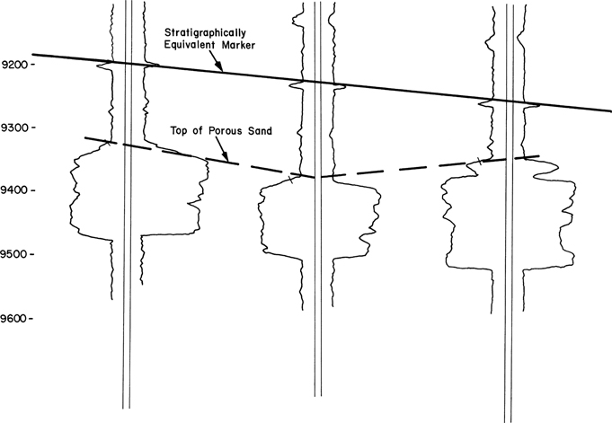
Figure 8-47 Electric logs from three wells. The upper stratigraphic marker conforms to true structure and is used to construct a map representing the true structural framework of the area. The top of the thick productive sand member does not conform to structure, but it represents a porosity top. It must be mapped separately to delineate the actual reservoir configuration.
It is common for the upper portion of a particular stratigraphic unit to be composed of nonreservoir-quality rock. This nonreservoir-quality rock is often referred to as a tight zone or tight streak. Although the top of the unit may represent an actual stratigraphically equivalent horizon, it is underlain everywhere by impermeable rock. Therefore, the structure maps prepared to interpret the true structure commonly cannot be used to evaluate the reservoir itself.
Once a structure map is completed, the next step is to prepare a top-of-porosity map for accurate delineation of the reservoir, and for later use in the construction of net hydrocarbon isochore maps. Two parameters are considered in evaluating the importance of separately mapping the top of porosity: (1) the thickness of the tight zone, and (2) the relief of the structure. A thick tight zone has a greater effect than one that is thin. Low-relief structures introduce greater error in delineating the limits of a reservoir than steeply dipping structures, particularly if the low-relief structure contains a bottom water reservoir.
Figure 8-48a shows a structure map and cross section for the 6000-ft reservoir. This unit consists of nonreservoir-quality rock in the upper 75 ft. The same reservoir is mapped on the top of the porous rock or porosity top in Figure 8-48b. Notice in cross section A-A′ that by mapping on the top of the unit, in which the upper 75 ft consists of nonreservoir-quality rock, the limit of the reservoir (gas/water contact) is extended beyond the true gas/water contact as mapped on the top of porosity (also see Figure 8-48c). Even though no net pay is assigned to the tight zone, the productive area of the reservoir mapped on the top of the nonproductive portion of the unit is larger. In turn, the volume of the reservoir is also larger than that mapped on the porosity top. In this case, the volume, based on net gas isochore maps, is larger by 32%. This added reservoir area (Fig. 8-48c) created by mapping on the top of the stratigraphic unit does not contain hydrocarbons and therefore is not productive; consequently, the volume of recoverable hydrocarbons based on this map is overestimated.
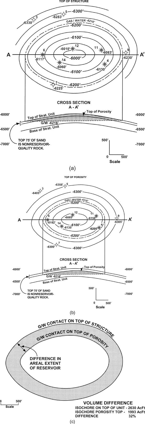
Figure 8-48 (a) Structure map on top of the 6000-ft unit, with a gas/water contact at a depth of −6216 ft, and cross section A-A′ illustrating (1) the top of the unit, (2) top of porosity, and (3) base of unit. (b) Structure map on the top of porosity for the 6000-ft unit, with the gas/water contact at a depth of −6216 ft, and cross section A-A′. (c) Mapping on top of structure versus top of porosity results in a 32% increase in volume.
The decision to prepare a separate map on the top of porosity, where the upper portion of a unit is not productive, needs to be made on a reservoir-by-reservoir basis. Depending on the geometry of the reservoir and thickness of the tight zone, the difference in volume between a map on the top of the unit and a map on the top of porosity may be too insignificant to warrant additional mapping. In Chapter 14, we discuss in greater detail the impact of nonproductive zones in isochore mapping.
Contour Compatibility—Closely Spaced Horizons
Structure maps on vertically close horizons should exhibit, in most cases, compatible contour configurations. In order to maintain compatibility during manual structure contour mapping of two or more vertically consecutive horizons, a completed map should be used as a guide for the next horizon to be mapped. The simplest way to do this is to lay the completed map under the base map for the next horizon to be mapped, and use it as a guide for contouring the new horizon map. This technique usually ensures that consecutively mapped horizons possess structural compatibility or contour compatibility.
Figure 8-49 illustrates the use of this technique and also shows the problems that can arise if vertically consecutive horizon maps are not overlaid during structure contouring. In Figure 8-49a, the completed structure map for Horizon A was used to guide the contouring of Horizon B. Notice the compatibility in the structural configuration of the two horizons. Figure 8-49b illustrates the kind of contouring errors that can arise when a completed map is not used to guide the structure contouring of another, vertically close horizon. Notice that in the area of good well control, the contours are similar to those in Figure 8-49a. The major problem occurs in the areas of limited control on Horizon B. Observe in Figure 8-49b that several contours on Horizon A actually cross contours of the same value on Horizon B (e.g., the −5950-ft contour), which incorrectly indicates a stratigraphic thickness between Horizons A and B of zero feet, as well as a crossing of the horizons. We know, however, from the available well data, that there are about 100 ft gross between these two horizons.

Figure 8-49 (a) Structure contour maps on Horizons A and B showing structural compatibility. The configuration of Horizon A was used to guide the contouring of Horizon B, especially in areas of limited or no well control. (b) An alternate interpretation of the structure contour map on Horizon B drawn independently and not taking advantage of the configuration of Horizon A, which has additional subsurface well control. A geologically impossible situation is shown; a contour of a given value (e.g., −5950) on Horizon A crosses a contour of the same value on Horizon B.
One contouring rule states that contours of the same value cannot cross on separately mapped horizons. If contours of the same value, mapped on different horizons, intersect or cross, then the interval between the two horizons would have zero or negative thickness, which is a physical impossibility. This is a serious mapping error that occurs because completed structure maps are not used to guide the contouring of other, vertically close horizons.
A major mapping bust is shown in Figure 6-11a and b in Chapter 6. In the situation shown, the two horizons are not vertically close (separated by 800 ft of section in the off-structure position) and yet the structure contour maps for the P5 and P7 Horizons cross in the up-structure position. To avoid such errors, we recommend that completed structure maps always be used to guide the contouring of other horizons, whether they are above or below the completed map.
Many software packages are designed to mimic this approach through conformal gridding. After a structure map has been made on one horizon, the software uses the shape of that horizon to guide the contouring of a nearby horizon while still honoring all of the control points of the second horizon (Thompson et al. 2017). This concept is also discussed in Chapter 2 under Conformable Geology and Multisurface Stacking.
Application of Contour Compatibility Across Faults
The method of contouring across faults using the vertical separation requires the structure (individual horizons being mapped) to have the same or similar attitude on opposite sides of the fault, as shown in Figures 6-5, 6-8, 8-10, 8-22, and 8-23. This means that the use of the technique requires structural compatibility, or contour compatibility, across the fault. For many tectonic settings, the compatibility of structural attitude across faults is more the rule than the exception; for others, it is not. Use of vertical separation for contouring across faults, shown earlier in this chapter, does have application on a worldwide basis in nearly every tectonic habitat, including some of the areas listed here.
Thin-Skinned Extensional Areas
Gulf of Mexico—onshore and offshore
West Coast of Africa— Gabon and Niger Delta areas
Crystalline Basement-Involved Extensional Areas
East African Rift area
North Sea
Red Sea
South America
Thin-Skinned Compressional Areas
Southern Mexican Ridges
South American Andes
Western United States and Canada
Diapiric Salt Tectonic Areas
Gulf of Mexico
North Sea
Northern German Salt Basin
Strike-Slip Fault Tectonic Areas
Western United States
The use of seismic data is very helpful in determining whether there is structural (contour) compatibility across faults in any area being worked (Figs. 7-37 and 7-38). To be a good interpreter and mapper, you must have a good understanding of the tectonic setting being worked and detailed knowledge of the individual structures being mapped. It is very important to know where to apply a particular technique, such as mapping across faults, and where the structure being mapped is an exception to the rule, thus requiring a different technique.
Exceptions to Contour Compatibility across Faults
Four key geological situations usually result in differing structural attitudes and display structural incompatibility across a fault:
Normal listric growth faults exhibiting large vertical separation;
Thrust or large reverse faults and large strike-slip faults;
Intermediate to late-stage strike-slip faults; and
Ramps relating to rapidly dying thrust faults.
A listric normal growth fault, depending on its vertical separation and the local amount of contemporaneous deposition, may or may not possess structural (contour) compatibility across the fault. Usually, the larger the fault, the less chance of compatibility. For example, Figure 7-37 shows a growth fault (Fault A) with compatible beds across the fault. However, Figure 8-50 illustrates a large growth fault (Fault A) that does not have compatibility from the upthrown to downthrown fault blocks of the main fault. Figure 8-51 is a cross section from the Gulf of Mexico that shows a fault with both characteristics. The structural attitude is compatible across the fault in the shallow section, gradually becoming incompatible with depth. There are several reasons for this change in structural attitude, including the activity of the large Miocene growth fault shown to the far left in the cross section. The seismic section in Figure 11-12 illustrates a faulted rollover anticline. Structural compatibility is lacking across the large fault on the left, which is the fault that formed the anticlinal structure on the right. On the other hand, all faults within the anticlinal structure do exhibit structural compatibility.
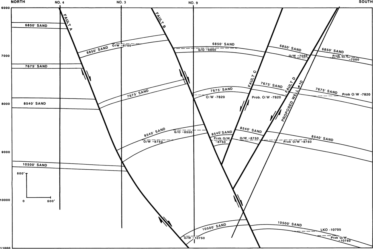
Figure 8-50 Observe the differing bed attitude upthrown and downthrown to the major growth Fault A. The rollover anticline, containing all the hydrocarbon accumulations, displays a compatibility of bed attitude across Faults B, C, and D. (Modified from Tearpock and Harris 1987. Published by permission of Tenneco Oil Company.)

Figure 8-51 The cross section from an offshore Gulf of Mexico field exhibits structural compatibility in the shallow section and structural incompatibility in the deeper section across the same normal fault. (Published by permission of the New Orleans Geological Society.)
Figure 8-26, discussed earlier, is an example of an area cut by a reverse fault that exhibits structural (contour) compatibility across the fault, so the vertical separation (the repeated section in this case) is used to map across the fault. In Figure 6-25, however, there are significantly different structural attitudes on opposite sides of the blind thrust fault; in this case, the technique of contouring the vertical separation across the fault cannot be used.
Vertical separation cannot easily be used to contour across a fault where there is no compatibility of structural attitude across the fault. For such structures, it is necessary to map each fault block separately and independently using the available well or seismic control. Each contoured fault block must be individually integrated with the fault surface map for the displacing fault to determine the upthrown and downthrown fault traces (Tearpock and Harris 1987).
Observe in Figure 8-50 that although the vertical separation mapping technique cannot be used across the major growth Fault A, the faulted hanging wall anticline that contains all the reservoirs does exhibit structural compatibility across all faults. Vertical separation must be used to map across all the faults that cut the rollover anticline in the hanging wall block of the major growth fault. This type of situation is quite common in both extensional and compressional areas. Major growth normal, thrust, or strike-slip faults may downdrop, thrust, or slide one fault block with respect to the other to such a degree that there is no compatibility of structural attitude across these major faults. However, the associated structures formed by these faults commonly possess structural compatibility across the faults within the structure. This is shown clearly in the cross section in Figure 8-50. Figure 8-22 is a structure map of a similar anticline downthrown to a very large growth fault (which is not shown on the map). Note the structural compatibility across the large fault (on the west), even though the vertical separation is about 1100 ft.
A good example of an area exhibiting both compatible and incompatible structural attitudes across faults, within the same field, is seen in the Cactus-Nispero Field in the Southern Zone, Mexico. Figure 8-52a is a structure map on the middle Cretaceous showing this salt-cored structure cut by both normal and reverse faults. Figure 8-52b and c are cross sections through the field, both of which are shown in plan view (F-F2 and G-G2) on the structure map. A careful review of the structure map and cross sections shows that the structure exhibits contour compatibility across most of the faults, and therefore the vertical separation should be used to map across these faults. Two areas provide major exceptions. In cross section F-F2, structural compatibility is lost across the reverse fault cutting Well No. C-87. On the structure map, the large normal fault just north of the salt body does not exhibit contour compatibility from the upthrown to downthrown blocks. To contour these two areas accurately, each block must be contoured separately and then integrated with the fault map for each associated fault.
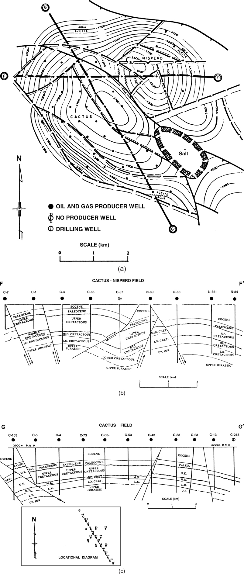
Figure 8-52 (a) Structure map of the Middle Cretaceous, Cactus-Nispero Field, Southern Zone, Mexico. The structure is a salt-cored structure cut by normal and reverse faults. (b) Geological cross section F-F′ through the Cactus-Nispero Field. (c) Geological cross section G-G′ through the Cactus Field. (From Santiago-Acevedo 1980. AAPG©1980, reprinted by permission of the AAPG whose permission is required for further use.)
Although many ramps relating to rapidly dying faults do not exhibit contour compatibility, some do. The complication here is that the vertical separation across the fault changes rapidly along the ramp, so the contour spacing on opposite sides of the ramp will be different.
All these examples stress the importance of understanding the 3D geometry of any structure being interpreted and mapped. The accuracy of the mapping depends on the use of the correct mapping techniques, which often depends on the geometry of the structure itself. Different techniques may be needed within the same field.
Mapping Techniques for Various Tectonic Habitats
In this section, we review the mapping techniques applicable to four major tectonic habitats and their associated hydrocarbon traps. These habitats include (1) extensional, (2) compressional, (3) strike-slip fault, and (4) diapiric settings. In addition to discussing the various types of hydrocarbon traps in each tectonic setting, we illustrate the fault surface map and the integrated contour construction of fault traces for each of the fault patterns observed in these settings, and present a field example where possible.
Extensional Tectonics
For extensional tectonics, we include nongrowth normal fault systems and detached listric growth fault systems, since both commonly occur together within this setting. In many areas of the world, hydrocarbons are trapped upthrown to normal faults. Important exceptions to this are found in the Gulf of Mexico and the Niger Delta, where hydrocarbons are commonly trapped downthrown as well as upthrown to normal faults. Also, reservoir-bearing rollover anticlines commonly occur in blocks downthrown to listric growth normal faults.
Faults are the primary trapping mechanism for hydrocarbons in extensional habitats, although four-way closures, unconformities, and stratigraphic traps are also important. Our primary discussion centers around five different types of fault patterns: (1) single nongrowth (structural) faults, (2) compensating, (3) bifurcating, (4) intersecting, and (5) growth fault systems.
The construction techniques for all fault patterns that exhibit structural compatibility across a fault are the same as those used for the working model (Fig. 8-21) to arrive at an integrated structure map. For the examples of each fault pattern, we show at least two mapped horizons that bound a stratigraphic interval of constant thickness. For the purpose of detailing the correct mapping techniques, the data for the examples are somewhat idealized. However, the techniques are applicable in both simple and complex petroleum geological mapping. Where possible, actual examples for each of the fault patterns are presented.
Compensating Fault Pattern.
Figure 8-53a shows the fault surface contour map for Faults A and B, which together represent a typical compensating fault pattern. If necessary, refer again to Chapter 7 and review the major aspects of this fault pattern. Several key points must be reemphasized here. First, the line of termination must be shown on the fault surface map; its importance will become clear as we review the structure maps on the 6000-ft and 7000-ft Horizons. Second, vertical separation is conserved across fault intersections. Observe that throughout the area where two faults are present (i.e., the area south of the line of termination of Fault B at Fault A in our example), Fault A has 100 ft of vertical separation and Fault B has a vertical separation of 200 ft. Only Fault A is present north of the termination line, and there its vertical separation is 300 ft.
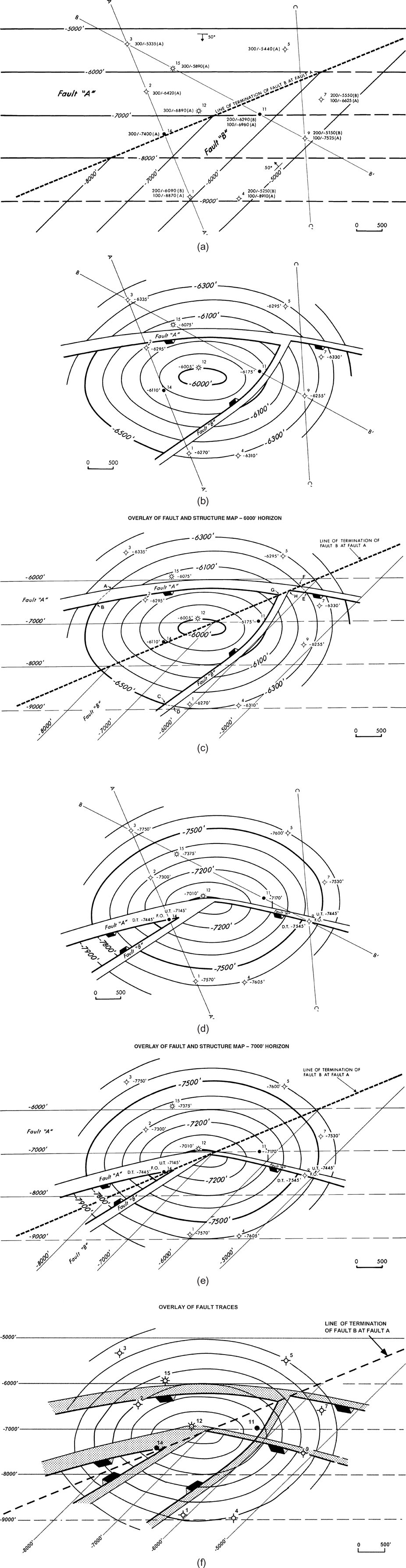
Figure 8-53 (a) Fault surface map for a compensating fault system including Faults A and B. (b) Integrated structure map on the 6000-ft Horizon. (c) Fault and structure maps (6000-ft Horizon) superimposed to illustrate the details of the integration technique. (d) Integrated structure map on the 7000-ft Horizon. Upthrown and downthrown restored tops in Wells No. 9 and 14 were used to aid in the structural interpretation. (e) Fault and structure maps (7000-ft Horizon) superimposed to show the accurate construction of the faulted 7000-ft Horizon map using the integration technique. (f) Overlay of fault traces for both the 6000-ft and 7000-ft Horizons. The figure shows that the intersections of all fault traces fall on the line of termination. The location of the fault intersections on any structural horizon can be predicted from the strike of the line of termination.
Figure 8-53b is a completed structure contour map on the 6000-ft Horizon. The structure is a faulted anticline. Figure 8-53c shows the fault surface map for Faults A and B superimposed onto the completed structure map for the 6000-ft Horizon. Using this figure, we review the construction of the upthrown and downthrown traces for each fault, the construction of the intersection of the two faults, and the proper horizon contour construction across each fault using the vertical separation (missing section from each wellbore).
Begin with the northern upthrown fault block and the −6200-ft contour, and follow its complete construction over the entire structure. The intersection of this structure contour with the fault contour of the same value defines the upthrown trace of Fault A at point A. The contour is projected through the fault, as if the fault were not there, and adjusted in the downthrown block by the amount of the vertical separation (300 ft) to become the −6500-ft contour. The intersection of this −6500-ft structure contour with the fault contour of the same value defines the downthrown trace of Fault A at point B. The −6500-ft contour downthrown to Fault A crosses the axis of the structure and intersects with the −6500-ft contour for Fault B at point C, defining the downthrown trace of Fault B at this location. The contour is now projected through Fault B, as if the fault were not there, and then adjusted by 200 ft (representing the vertical separation for Fault B) in the upthrown block of Fault B to become the −6300-ft contour. This −6300-ft structure contour intersects the −6300-ft fault surface contour at point D, defining the upthrown trace of Fault B at this location. This contour once again crosses the axis of the structure, this time on the eastern side of the anticline, and intersects with the −6300-ft contour of Fault A at point E, defining the downthrown trace of Fault A. Project the contour through the fault gap of Fault A and adjust its value by 100 ft for the vertical separation at point F, defining the upthrown trace of Fault A. Finally, this contour continues in the upthrown block of Fault A until it intersects with point A, which was our starting point. This technique is applied for each structure contour on the map to arrive at the integrated structure map shown.
The heavy dashed line (Fig. 8-53c) striking southwest-northeast is the line of termination of Fault B at Fault A. The intersection of the fault traces on the completed structure map for both faults falls on this line of termination. For this map, there are two trace intersections: (1) the intersection of the downthrown traces of Faults A and B shown at point G, and (2) the intersection of the upthrown trace of Fault B with the downthrown trace of Fault A shown at point H. Since all trace intersections must fall on the line of termination, it is very important to place this line on the fault surface map. By following the line, we can predict the location of the fault intersections for other horizons either shallower or deeper in the subsurface, because all intersections must fall on this line. Observe that north of the line of termination, only Fault A is present, with a vertical separation of 300 ft, whereas south of the line, both Faults A and B are present, with vertical separations of 100 ft and 200 ft respectively. Take a minute and test the additive property of faults around the fault intersection on the completed structure map.
This construction technique of integrating the fault and structure maps removes all the guesswork with regard to: (1) fault trace construction; (2) the location of all faults on the structure map; (3) the location of all fault intersections; and (4) the width of the fault gaps. The integration of the two maps constructs all these features automatically without the need for guesses or estimates. Take one or two additional structure contour lines and go through the same procedure just described to make sure you fully understand the technique for integrating a fault map with a structure map.
Figure 8-53d is a structure map on the deeper 7000-ft Horizon, and it shows that the faults have migrated with depth. The technique of construction is exactly the same as presented for the 6000-ft Horizon. In Figure 8-53e, we again superimpose the fault map onto the completed structure map. Choose several structure contours and follow each across the mapped area to review the construction techniques as discussed for the preparation of the completed structure map for the 6000-ft Horizon.
Finally, the completed fault traces for both the 6000-ft and 7000-ft Horizons, and the general trend of the structure contours is superimposed onto the fault map for Faults A and B in Figure 8-53f. Looking at each set of fault traces (those for the 6000-ft and 7000-ft Horizons), can you detect any difference between them? Use 10-point proportional dividers or an engineer’s scale to measure the width of the fault gap for Fault A on both horizons. Notice that the gap is wider for Fault A on both sides of the line of termination on the structure map for the 7000-ft Horizon, when compared with the fault gap on the structure map for the 6000-ft Horizon. Remember the general rule of fault gap width presented earlier. A fault dipping up-dip (in the opposite direction of bed dip) will have a narrower fault gap than a fault of the same or similar vertical separation dipping down-dip (in the same direction as the bed dip). Notice that Fault A on the 6000-ft Horizon is on the northern side of the structural axis and is dipping generally in the opposite direction to the formation. On the deeper structure map for the 7000-ft Horizon, Fault A has crossed the axis of the structure and is now dipping more or less in the same general direction as the formation. Therefore, the fault gap is wider as mapped on the structure map for the 7000-ft Horizon.
With the technique of integrating the fault and structure maps, this change in fault gap width is automatically built into the integration. It is unlikely that such a change in gap width could have been intuitively incorporated into the completed structure contour maps had the fault and structure map integration technique not been used. For this example, the change in gap width is significant, but depending on the configuration of the structure and the geometry of the fault, the change in width can be minor. Let the integration technique be the tool used to establish fault gap widths.
The completed structure map in Figure 8-22 illustrates two compensating faults to the large down-to-the-east normal fault. Fault surface maps were prepared for each fault, and they were integrated with the structure map to arrive at the completed map.
Look at the completed structure map in Figure 8-54a. What type of fault pattern is represented by the intersection of Faults A and D? Is it a compensating fault pattern, or is it a mapping error? Can you find any other errors on this map?
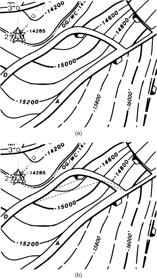
Figure 8-54 (a) Compensating fault system or mapping bust? (b) Implied strike of Fault D (dashed) based on where the −14,900-ft′ contour intersects the fault trace.
Bifurcating Fault Pattern.
The fault map in Figure 8-55a shows a fault contour map for Faults A and A-1, which together form a bifurcating fault pattern. Refer again to Chapter 7, if necessary, to refresh your memory on the characteristics of a bifurcating fault pattern. Figure 8-55b is the completed structure map on the 6000-ft Horizon. Figure 8-55c shows the fault surface map for Faults A and A-1 superimposed onto the structure map for the 6000-ft Horizon. Choose several structure contours upthrown to Fault A and go through the integration technique to check the position of the fault traces and the fault intersections, the width of the fault gaps, and the contour construction for the 6000-ft Horizon across the two faults.
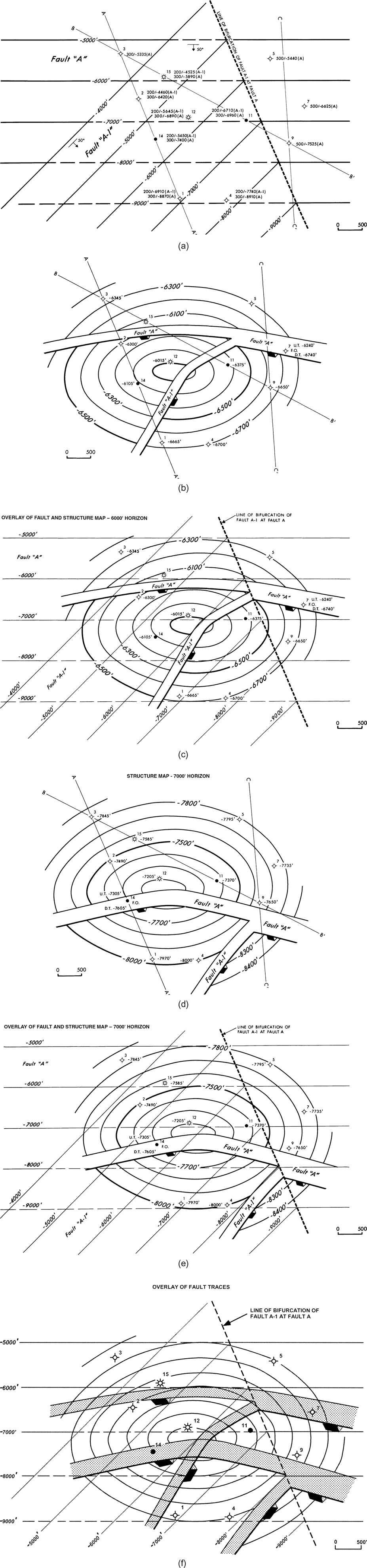
Figure 8-55 (a) Fault surface map for a bifurcating fault system including Faults A and A-1. (b) Integrated structure map on the 6000-ft Horizon. (c) Fault and structure maps (6000-ft Horizon) superimposed to show the accuracy of the integration technique: to position the fault traces and intersections and to determine the width of the fault gap. (d) Integrated structure map for the 7000-ft Horizon. (e) The fault map superimposed onto the 7000-ft structure map. (f) Overlay of fault traces on both the 6000-ft and 7000-ft Horizons. As with the compensating fault pattern, all intersections of fault traces fall on the line of bifurcation.
Fault traces are relatively easy to delineate when there are a number of structure contours intersecting fault contours, as in the case shown in Figure 8-55; however, in areas where fault contours are semiparallel to the structure contours, it is more difficult to delineate the fault traces. In these situations, you must interpolate depth values to precisely delineate the position of the fault traces.
Figure 8-55d is the completed structure map on the 7000-ft Horizon. Figure 8-55e shows the fault surface map superimposed onto the structure map. Observe that the trace intersections for Faults A and A-1 fall directly on the line of bifurcation. Figure 8-55f shows the fault traces, as seen on the completed structure maps for both the 6000-ft and the 7000-ft Horizons with the fault surface map superimposed. Notice how the fault intersection migrates from north to south along the path of the line of bifurcation. Also observe that the width of the fault gap for Fault A is wider on the structure map for the 7000-ft Horizon than it is on the 6000-ft Horizon structure map. This occurs here for the same reason discussed for the compensating fault example.
Figure 8-56 is a portion of the structure map on the Nodosaria Marker, and Figure 8-57 is a portion of the U Sand structure map from the offshore Gulf of Mexico. Both figures show good examples of the mapping of a bifurcating fault system. The fault system in Figure 8-56 actually has two bifurcations. Take a minute to check the construction of these completed maps in the area around the bifurcations by applying the additive property of faults.
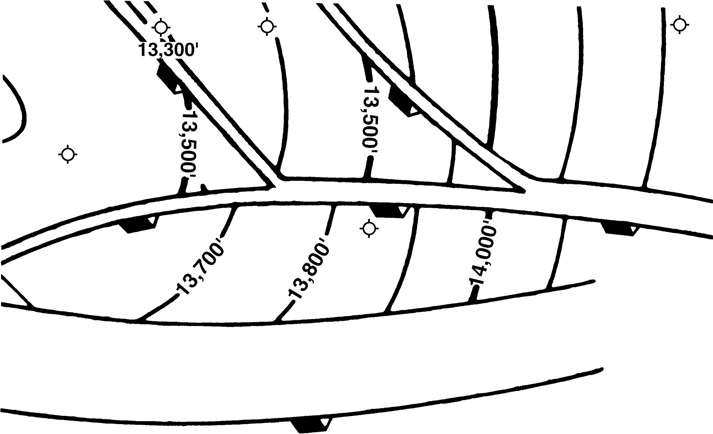
Figure 8-56 Portion of the structure map on the Nodosaria Marker illustrating a bifurcating fault system. (Published by permission of the Lafayette Geological Society.)
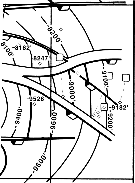
Figure 8-57 Example of a bifurcating fault system from the offshore Gulf of Mexico. (Published by permission of the New Orleans Geological Society.)
Now we revisit Figure 8-54. Both of the faults that merge dip in the same direction, so this is a bifurcating system. The gap for the fault that extends to the east of the point of merger would be expected to be larger than the gap on either of the two faults, thus reflecting the additive property of faults. However, the gap is much narrower than that of either fault. Actually, the gap is of the size expected if this were a compensating fault system, so the interpretation is incorrect. The only way that the gap could be correctly constructed to be so narrow is if the fault were to abruptly become almost vertical right at the point of merger of the two faults, and that is certainly unreasonable. In further review of the map, we can use the implied strike technique (Tearpock et al. 1994) on the northern fault, whose trace bends sharply. The implied strike technique takes advantage of the fact that at each point where a structure contour intersects a fault trace, we know the depth of both the horizon and the fault surface. Connecting the depth points from the fault surface along one or more fault traces allows us to approximate the fault surface map that is implied by the fault trace on the structure map. Using the two points where the −14,900-ft contour intersects the downthrown fault trace of Fault D and the one point where the −14,900-ft contour meets the upthrown fault trace of Fault D, we see that the implied fault strike of Fault D abruptly changes (Fig. 8-54b). Is such a sharp bend reasonable for a normal fault? Finally, structural compatibility is lacking across the northern fault. Notice that the vertical separation decreases rapidly from 600 ft to 300 ft in an easterly direction. The poor contour compatibility is apparently due to the interpreter honoring that displacement. Again, do you think that this abrupt change in vertical separation is reasonable along this single fault, or could something else be happening? Notice that it occurs near the sharp bend in the implied fault surface. Could Fault D actually be two faults?
Intersecting Fault Pattern.
Figure 8-58a illustrates a typical intersecting fault pattern composed of Faults A and B. Cross section A-A′ is shown in Figure 8-58b. In the section in Chapter 7 dealing with the intersecting fault pattern, the fault surface maps were contoured with the assumption that neither fault surface was offset (Fig. 8-58b). In other words, the two faults were considered contemporaneous rather than of two different ages. The fault traces for the structure maps shown in Figure 8-58 were constructed with this assumption. Notice, however, in Figure 8-58c through g, that all the fault traces are offset. Figure 8-58d shows, for example, that although the fault surfaces themselves are not offset, the fault traces on the completed structure maps show significant offsets for all the fault traces at the fault intersections. The positions of the offset traces are accurate for the constructed fault surface maps. If the faults are of two different ages, however, then the completed maps are subject to error around the intersection. If the faulting is contemporaneous, then the traces are accurate as shown on the completed structure maps.
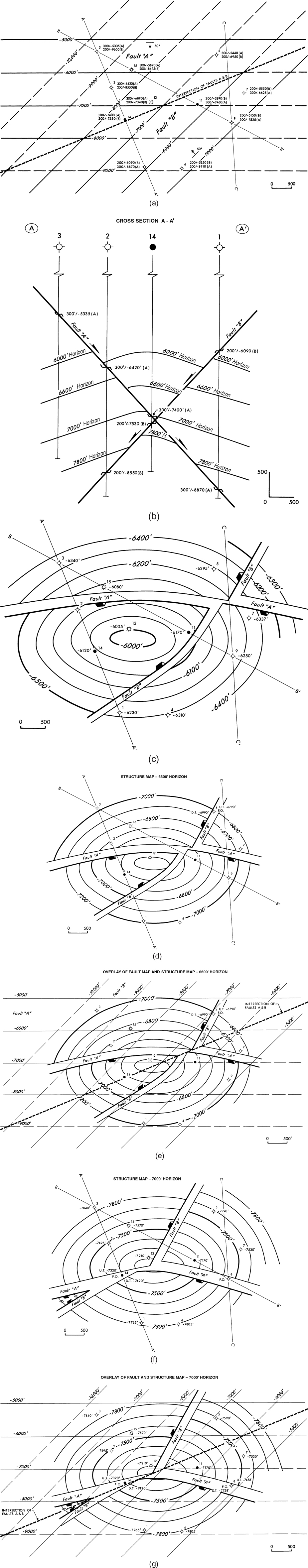
Figure 8-58 (a) Fault surface map for an intersecting fault system including Faults A and B. Fault B does not terminate at the line of intersection. (b) Cross section A-A′ illustrates the shortcut method of constructing the fault map as if the fault surfaces are not offset. (c) Integrated structure map on the 6000-ft Horizon. (d) Completed structure map on the 6600-ft Horizon. Observe that all fault traces are offset at the intersection. (e) Fault surface map and the structure map on the 6600-ft Horizon superimposed to show the accuracy of fault trace construction. (f) Completed structure map on the 7000-ft Horizon. (g) Overlay of the fault surface map and the 7000-ft structure map. Notice that all fault trace intersections fall directly on the line of intersection.
Compare the completed structure maps in Figure 8-58d and f. There is a pronounced change in the configuration of the fault traces shown on these two maps. The change is the result of the intersecting geometries of the two horizons with Faults A and B at different depths. Without the integration of the fault and structure maps, the accurate delineation of these fault traces, particularly for the 7000-ft Horizon, would be difficult, if not impossible.
Finally, observe that all the fault trace intersections fall on the line of intersection. In this case of two intersecting faults, there are four fault trace intersections (Fig. 8-58e and g). This construction again emphasizes the necessity of placing the line of intersection on the completed fault maps.
Where faults of two different ages intersect, the construction of accurate fault surface maps showing the offset of an earlier fault by a later one may require seismic data to determine the relative ages of the faults. Also, a graphical solution to the construction of the fault surfaces and their effects on stratigraphic horizons can be undertaken. A graphical technique is presented by Dickinson (1954). The method is not detailed here; however, if it is absolutely necessary to prepare precise fault and structure maps reflecting the accurate geometry of intersecting faults of different ages, then the Dickinson method should be considered. In most cases, the relative ages of different intersecting faults can be determined if reasonable quality seismic data is available.
Figure 8-59, from Dickinson’s paper, shows a completed structure map for a horizon above a deep-seated salt dome in Texas. Such a complex intersecting fault pattern is not uncommon in areas of salt tectonics. In this example, Faults 3 and 5 are intersecting. A test was planned for the upthrown block to the east. In order to test the block at an optimum structural position, it was necessary to accurately locate the position of the intersection of Faults 3 and 5, so the graphical solution outlined by Dickinson was used to prepare the fault and structure maps.

Figure 8-59 Structure contour map over a deep-seated salt dome in Texas illustrating several intersecting faults. (From Dickinson 1954. AAPG©1954, reprinted by permission of the APPG whose permission is required for further use.)
Intersecting faults of different ages are quite common in certain geological settings, especially where the stress field has shifted over time. Ferrill et al. (2009) illustrate this very well from the Jean d’Arc Basin offshore Newfoundland, which has a set of early faults that formed when the least principal stress was east-west. These faults strike predominantly north-south. During a later phase of rifting, the least principal stress was north-south and the faults strike predominantly east-west. Contemporaneous intersecting normal faults tend to have similar strikes as they form in the same regional stress field. Intersecting normal faults of different ages may have similar or different strikes, depending on the regional stress field when the faults formed.
In addition to the intersecting normal faults, some areas around the world, such as western Texas, California, southern Oklahoma, the North Sea, and the southern zone of Mexico, contain intersecting normal and reverse faults. The Dickinson method is also very helpful in developing a structural picture of these intersecting faults. For many situations, however, particularly those involving small faults, the shortcut method of assuming contemporaneous faulting, shown earlier in this section, is often adequate for the construction of the fault surface maps and completed structure maps.
We cannot leave this subject of intersecting faults without covering an important misunderstanding with regard to intersections of fault traces on completed structure maps. There seems to be a popular belief that where two faults of different ages intersect, the fault trace of the intersected or older fault is not offset on a completed structure map, as shown in Figure 8-60. We strongly emphasize that this idea is incorrect for most cases. The traces of each of the intersecting faults on any mapped horizon always offset, except in two special cases. These exceptions, which are covered in detail by Dickinson (1954), occur where (1) the beds are horizontal, the faults intersect at right angles, and the movement on both faults is entirely dip-slip (Fig. 8-60); or (2) the intersection of the (older) intersected fault and the mapped horizon is parallel to the direction of slip on the younger fault. Obviously, these two exceptional situations are rare. In both cases, the trace of the (older) intersected fault will not be offset, but the trace of the (younger) intersecting fault will be. So, if neither of the faults traces is offset, then the structure map is incorrect (no exceptions). These guidelines apply to intersecting normal faults and intersecting reverse faults. Dickinson (1954) also discusses intersections of normal faults with reverse faults.

Figure 8-60 Block model and map view of intersecting normal faults in horizontal strata. Fault dip is 60 deg and the movement is all dip-slip. This result is only applicable in this special case of right-angle faults and flat beds. (Modified from Dickinson 1954. AAPG©1954, reprinted by permission of the APPG whose permission is required for further use.)
A structure map with intersecting faults showing the intersected (older) fault traces with no offset must meet one of the two special cases, or it is constructed incorrectly. Usually, this type of error occurs because (1) the interpreter does not understand the relationships of intersecting fault construction, or (2) no fault surface maps were prepared and used to integrate with the structure map to arrive at an accurate solution for the intersecting faults. Figure 8-61 is a portion of a completed structure map with an intersecting fault pattern. A review of the map shows that only one fault trace is offset for each pair of crossing faults, so the map is immediately suspect. Consider the two exceptions to the rule that both traces should be offset. The map shows that the beds are dipping, so exception (1), based on horizontal beds, does not apply. However, exception (2) might be valid if the movement on Fault B was in exactly the same direction as the trace of Fault A. However, we cannot determine that. The only way to determine the accuracy of the fault traces is to have a fault surface map and integrate it with the horizon map. However, for the map in Figure 8-61, the fault traces were prepared showing no offset for the assumed older Fault A.
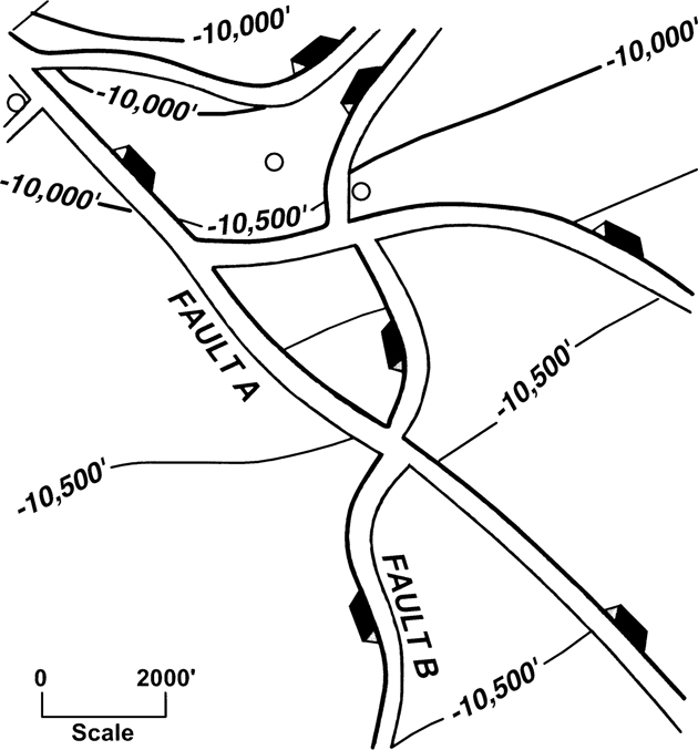
Figure 8-61 Portion of a structure map showing incorrectly interpreted and constructed intersecting faults.
If a pair of intersecting fault traces is shown on a completed structure map with neither trace offset and the traces resembling a cross (Fig. 8-62), the construction is incorrect. Such errors as the ones shown in Figures 8-61 and 8-62 can place suspicion on the rest of the structural interpretation.

Figure 8-62 Completed structure map showing several intersecting faults with each of the trace intersections forming a “cross.” (The final construction is incorrect. No fault traces are offset.)
If the area you are working is complexly faulted with intersecting faults and extreme accuracy is required, it is advisable to become familiar with the Dickinson method for resolving the geometry of fault intersections.
Combined Vertical Separation.
In Chapter 7, we discussed the combined vertical separation that results where two faults of different ages intersect. In Figure 8-60, the zone of combined vertical separation at a given horizon is shown in map view for this example of intersecting normal faults. It is the area between points J, E′, N, and M. A well drilled within this zone will cross only one of the two intersecting faults, but the interval shortening, or missing section, is equal to the sum of the vertical separations for both faults. For this example, the earlier fault has a vertical separation of 150 ft and the later fault is 250 ft; therefore, the vertical separation for a fault in the area of combined vertical separation is 400 ft.
Growth Faults.
A growth fault is a special type of normal fault. A growth fault is a normal fault that is contemporaneous with deposition, and it is often referred to as a syndepositional fault. There are several primary characteristics of growth faults.
They are commonly arcuate in lateral extent and concave toward the basin.
Fault dip typically decreases with depth, commonly becoming a bedding plane fault at depth (Chapter 11). We refer to this shape as listric, based on the Greek word listron, or shovel, due to its curved shape in cross section. However, fault dip can locally increase with depth (see the section Compaction Effects along Growth Normal Faults, in Chapter 11).
The vertical separation for the fault normally increases with depth. Displacements of several thousands of feet or kilometers are not uncommon. Growth faults can also include displacements that decrease with depth as well (see Chapter 11).
The time-stratigraphic intervals in the hanging wall blocks are thicker than the equivalent intervals in the footwall blocks (see the section Estimating the Vertical Separation for a Growth Fault, in Chapter 7).
A rollover anticline commonly develops in the hanging wall fault block of a growth fault as a result of collapse of the hanging wall block.
Secondary faulting within the hanging wall block is normally associated with growth faults. These faults can be synthetic (dipping parallel to the master fault) or antithetic (dipping toward the master fault).
A majority of growth faults dip toward the current basin or the paleo-basin and strike parallel or semiparallel to the coastline. However, growth faults can dip in any direction, including toward the margin of the basin. Along strike, most growth faults are generally concave in the direction of dip.
Faults are not perfect planar surfaces of slip; they generally have undulations of some type. As two fault blocks slip past one another, there must be deformation in at least one fault block, because rocks are not strong enough to support large voids. This is the main reason why many major rollover folds exist within the hanging wall fault blocks, formed by bending of the fault blocks as they slip over nonplanar (listric) fault surfaces. This mechanism of folding is called collapse folding (Hamblin 1965) (see Chapter 11 for details of the collapse mechanism). The rollover anticline, associated with listric growth faults, is one of the most widely recognized petroleum-producing folds, as seen in such areas as the Gulf of Mexico, Brunei, and the Niger Delta.
For contouring purposes, the hanging wall and footwall may or may not have structural compatibility across a growth fault. The primary factors are the vertical separation of the fault and the amount of deposition in the downthrown block. Usually, the larger the fault, the less the compatibility. If structural compatibility does exist, the vertical separation can be contoured across the fault. If compatibility is absent, then each fault block must be contoured separately. At times, only the upthrown or downthrown block of a growth fault is mapped, usually because (1) good control or correlation is lacking across the fault, or (2) only one block is productive and that is the only block mapped.
Figure 8-63 is a structure map on the G Sand in East Cameron Block 270 Field, Gulf of Mexico. This field is productive from 19 separate horizons trapped both upthrown and downthrown to the west-dipping growth Fault A. Rollover into Fault A has formed a north-south trending anticline, which is the primary hydrocarbon trap. This field has produced more than 38 million barrels of oil and condensate and nearly 1 trillion cu ft of gas.
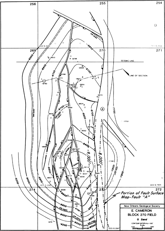
Figure 8-63 Structure map on the G Sand Unit, East Cameron Block 270 Field, Gulf of Mexico. A portion of the fault surface map for Fault A is superimposed on the structure map. The primary hydrocarbon trap is a faulted rollover anticline formed in response to Growth Fault A. (Published by permission of the New Orleans Geological Society.)
Superimposed on the southern half of the structure map is a portion of the fault surface map for Fault A from −8000 ft to −9000 ft. The structure contours drawn upthrown and downthrown to the fault, in this area, indicate reasonable compatibility in structure across this growth fault, which has a vertical separation of about 800 ft at this level. The existence of this structural compatibility does not, however, ensure such compatibility along fault strike nor with depth (recall the cross section in Figure 8-51). Notice that the rollover anticline is complexly faulted with secondary synthetic and antithetic faults. Although the fault maps for these faults are not published, it is easy to recognize that there is good structural compatibility across all the secondary faults; therefore, the vertical separation must have been used to contour across these faults.
One final note on growth faults. It is commonly observed that the most productive interval in a growth fault complex is the stratigraphic section deposited during the most active fault movement. Therefore, when prospecting around growth faults, it is important to understand the history of the fault movement. The technique of plotting a growth fault’s history, the Multiple Bischke Plot Analysis (MBPA) discussed in Chapter 13, is most helpful in evaluating the fault history and its potential for hydrocarbon accumulations.
Diapiric Salt Tectonics
A diapir is a mass of rock that has flowed ductilely and appears to have discordantly pierced or intruded overlying rocks and sediments (after Jackson and Talbot 1991). The word comes from the Greek verb diaperein, meaning “to pierce,” and was first used in the Carpathian Mountains of Romania. The most common use of the word is in association with salt and shale masses. Although this may not be the best term to describe a salt body or to correctly describe the motion of salt movement, it is in common use. Most salt diapirs probably formed by a mainly lateral movement of the salt into the diapir, with the movement being caused by differential loading upon the salt layer (Jackson and Talbot 1991; Diegel et al. 1995; Hudec and Jackson 2007), often called down building. In other words, the sediments move down into the salt, forcing the salt upwards, often forming a tear-shaped salt body (Fig. 8-72). The diapir increases in relief by growing downward relative to the sedimentary surface as the base of the sediments subsides into the mobile salt. Actual upward movement may be minimal for many domes. The extent of upward movement depends in part on the buoyancy of the salt mass and the strength of the overburden.
Diapiric salt masses are associated with large accumulations of hydrocarbons in many areas around the world, including the U.S. Gulf Coast, the southern zone of Mexico, Gabon, Senegal, the Canadian Arctic, the North Sea and adjacent Europe, Romania, the Zagros Mountains of Iran, and the Ukraine. These salt domes are commonly structurally and stratigraphically very complex. They come in all shapes and sizes from small, needle-like spines less than 2000 ft across, such as the Rabbit Island Salt Spine (Fig. 8-64), to very large salt massifs such as the Marchand-Timbalier-Caillou Island Salt Massif, which is more than 27 mi long and 13 mi wide at a depth of 20,000 ft (Fig. 8-65). Regardless of the actual size of the salt mass, most are associated with significant quantities of hydrocarbons. For example, the Rabbit Island Field has estimated reserves of 1.5 trillion cu ft of gas and 55 million barrels of condensate and oil. The fields associated with the Marchand-Timbalier-Caillou Island Salt Massif have combined ultimate reserves of over 500 million barrels of oil. Figure 8-66 shows the extent of salt structures in the northwestern Gulf of Mexico and adjacent interior basins. Salt masses in the Southern Permian Basin of the North Sea area are shown in Figure 8-67. Notice the general clustering of salt pillows versus piercement salt bodies.
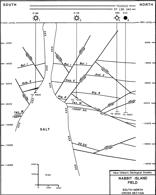
Figure 8-64 Cross section showing the needle-like Rabbit Island Salt Spine, which is less than 2000 ft across to a depth of about 7000 ft. (Published by permission of the New Orleans Geological Society.)
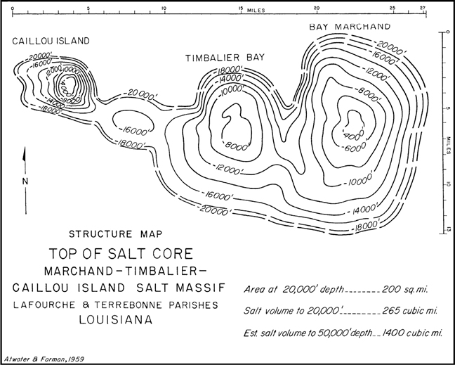
Figure 8-65 Structure map on the top of the Marchard-Timbalier-Caillou Island Salt Massif. (From Atwater and Forman 1959. AAPG©1959, reprinted by permission of the APPG whose permission is required for further use.)
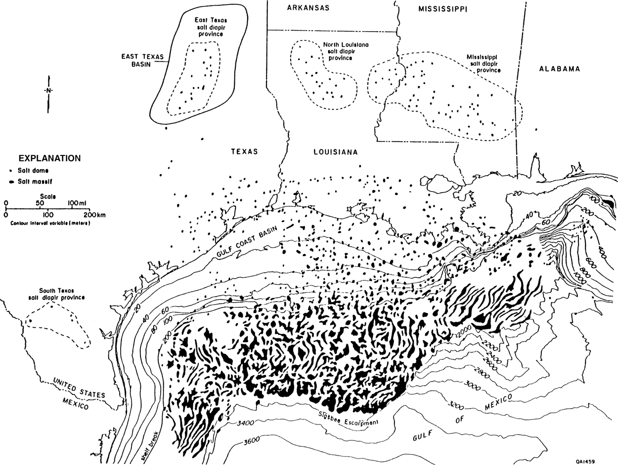
Figure 8-66 Salt structures in the Gulf of Mexico and adjacent interior basins. (From Seni and Jackson 1983. AAPG©19831983, reprinted by permission of the AAPG whose permission is required for further use.)
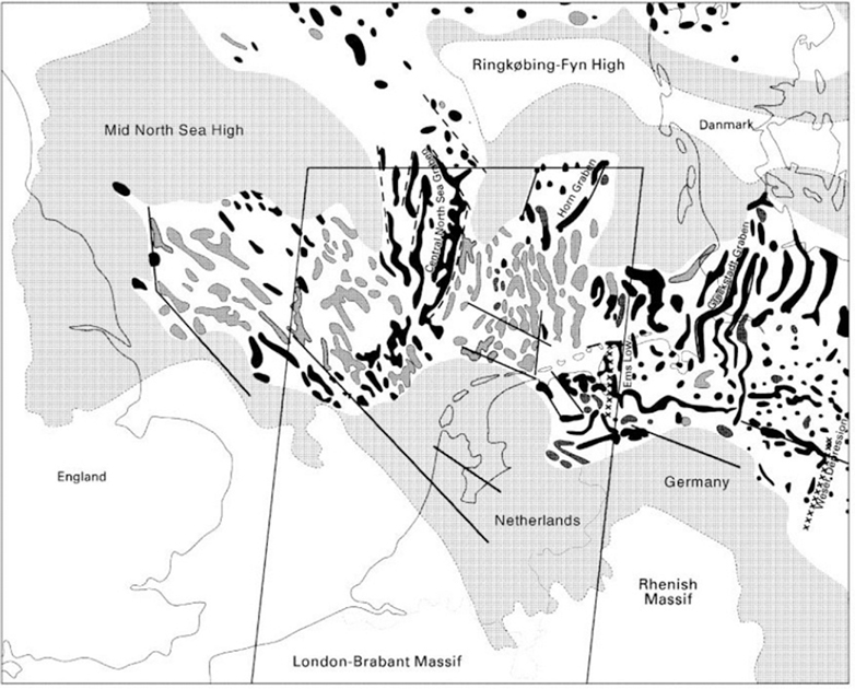
Figure 8-67 Map of salt pillows and piercement salt bodies in the Southern Permian Basin, North Sea Area. (From Remmelts 1995. AAPG©1995, published by permission of the AAPG whose permission is required for further use.)
An important development in petroleum exploration has been the recognition during the past 35 years that some irregular salt masses are sheets of salt that are detached from the source layer (Diegel et al. 1995). The salt often rides up ramps and forms sheets on different structural layers. Their size varies from small to hundreds of square miles in area. Typical sequences of strata and trapping structures exist beneath these salt sheets, and significant discoveries have been made.
Several types of normal faulting are commonly associated with most diapirs, as well as with many deep-seated salt structures. If the regional stress field is nearly isotropic, the normal faults develop in an outward radiating pattern from the salt structure, and these are called radial faults. If the regional stress field is more anisotropic, or the structure exhibits a variable growth history in different areas around the dome, the fault pattern may have a more preferred orientation, resulting in peripheral faults that are parallel to the face of the salt or ride down the flank of the salt. Rowan et al. (1999) discuss faults associated with various salt structures in much more detail.
Growth of a salt structure can develop in different stages. Graben blocks often form in the sediments over the salt mass due to extension. The dip of associated faults can be toward the dome as well as away from it. Although not directly associated with the salt dome development, regional growth faults are often found on or near salt structures. In certain areas of the world, salt diapirs are associated with reverse faults.
Hydrocarbon Traps.
Salt structures have an extremely varied and complex geometry resulting in numerous types of hydrocarbon traps. Any single salt structure may have more than one type of trap, depending on the history of the salt structure and surrounding sediments. Figure 8-68 (Halbouty 1979) shows an idealized section through a salt dome illustrating the more common types of hydrocarbon traps, including (1) a simple domal anticline, (2) graben fault traps over the dome, (3) porous caprock (limestone or dolomite), (4) up-dip pinchouts of permeable units, (5) traps beneath an overhang, (6) traps against the salt itself, (7) unconformities, (8) traps along faults downthrown away from the dome, and (9) traps along faults downthrown toward the dome. Fault traps like 8 and 9 can also be considered first-fault out-of-the-basin type traps. In addition to the traps shown in Figure 8-68, radial and peripheral faults also serve as excellent hydrocarbon traps.
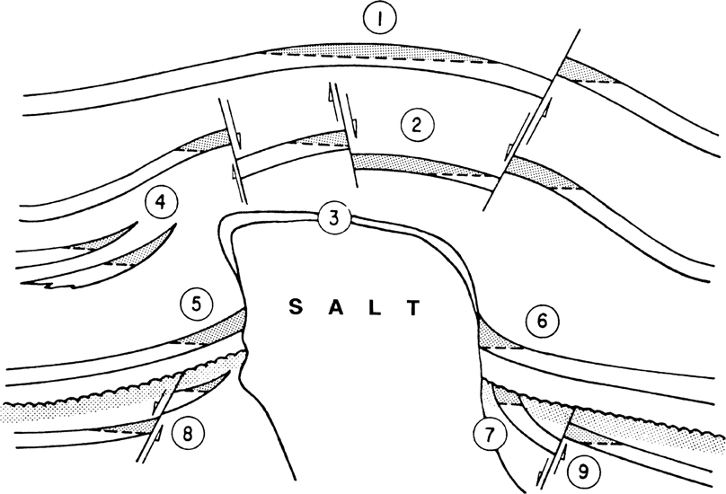
Figure 8-68 An idealized diapiric salt structure showing common types of hydrocarbon traps. (From Salt Domes, by Michel T. Halbouty. Copyright 1979 by Gulf Publishing Company, Houston, Texas. Used with permission. All rights reserved.)
Considering their complexity, salt structures require very precise interpretation and detailed mapping in order to exploit all the hydrocarbon potential. When working with salt-related structures, maps are needed for the salt itself and for salt/sediment, salt/fault, and fault/sediment interfaces, in addition to associated unconformities and top of shale, if present.
Contouring the Salt Surface.
No special techniques are required to contour the salt surface. The key to making a good salt map is having sufficient data. Typically, only a limited number of wells penetrate salt, and commonly the quality of seismic data near steeply dipping salt is poor. Figure 8-69 is the salt surface contour map for Main Pass Block 299 Field, which is of special interest because the salt dome has an overhang on the south and southwest flanks. Notice how the contours under the overhang are dashed, making the map easier to use when preparing structure contour maps, as well as making the salt map easier to read. Some of the deviated wells were drilled to traps beneath the overhang.
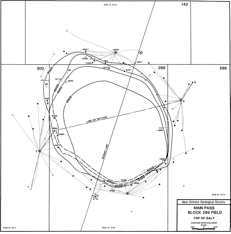
Figure 8-69 Surface of salt, Main Pass Block 299 Field, Offshore, Gulf of Mexico. Observe the dashed contours to clearly illustrate the salt overhang. Some deviated wells extend beneath the overhang. (Published by permission of the New Orleans Geological Society.)
Although the steep flanks of salt bodies are frequently poorly imaged on seismic data, there are other geophysical techniques that can provide additional data to assist in mapping a salt body. A salt proximity survey can consist of either a source above the salt and receivers in a well near the salt (e.g., Barker and Guzman 1992; Li et al. 2003; O’Brien 2004; Lou et al. 2012). The technique takes advantage of difference in velocity between salt and sediment to identify the location of the salt face. Another version of a salt proximity uses a source exterior to the salt body and receivers in a well within the salt. This arrangement is technically more challenging and frequently identifies only a small segment of the salt body (O’Brien 2004). An additional geophysical technique is a walkaway or walkaround vertical seismic profile (VSP) (Barker and Guzman 1992). These surveys can record reflections from the salt face that are not recorded on some surface seismic. In addition, properly designed conventional 3D seismic surveys with very long offsets can do an excellent job of delineating a very steeply dipping salt flank (e.g., Figure 1 in Hartman et al. 2017). Data from all of these geophysical sources, where available, should be combined with well log data to make the most accurate map of the salt surface possible (Li et al. 2003).
Salt/Fault Intersection.
Figure 8-70a illustrates the method for contouring the intersection of a salt mass and a fault. The technique is basically the same as that presented earlier for contouring the upthrown or downthrown traces of a fault. The salt/fault intersection occurs where the structure contours on the salt intersect the fault contours of the same elevation. Like all intersecting surfaces presented in map view, the salt/fault intersection should be delineated as shown in the figure. This line of intersection can serve as a directional guide for planning a deviated well that tests potential reservoir units in the structural trap between the surfaces.

Figure 8-70 (a) Integration of the contour maps on the salt surface and on Fault A delineates the intersection of the fault with salt. (b) Integration of the contour maps on the salt surface and on the structure contours for the 8000-ft Horizon. The salt/sediment boundary is located where the salt contours intersect the fault contours of the same elevation. (c) Completely integrated structure map on the 8000-ft Horizon, Reservoir A, in the southeast portion of this piercement salt structure. This oil reservoir is bounded to the north and west by salt, to the east by Fault A, and to the south by an oil/water contact at a depth of −8605 ft.
Salt/Sediment Intersection.
The salt/sediment intersection represents the termination of a sedimentary surface against the salt mass. This interface is important for two reasons: (1) it often serves as the seal for the trapping of hydrocarbons; and (2) it delineates the limit of the potentially productive hydrocarbon-bearing horizon. Figure 8-70b shows a portion of a salt contour map (same as in Figure 8-70a) and the line of termination of the 8000-ft Horizon against the salt. The termination of the horizon occurs where the structure contours intersect salt contours of the same elevation. The termination line bends sharply above 800 ft. This was located accurately by integrating interpolated contours on the two surfaces.
In some cases, sediments continue all the way to the salt face as with the shallow horizons, as illustrated in Figure 8-72. In these cases, the structure map on the surface of the salt can be integrated with the structure map of the reservoir to identify the termination of the reservoir unit. In other cases, the salt face is encased in a “sheath” of shale and impermeable rock, as at White Castle dome (Johnson and Bredeson 1971) and the reservoir sands terminate against this sheath, prior to reaching the salt. In still other cases, the salt structure was a positive feature during deposition and porous sediments pinch out prior to reaching the salt face. This situation is common in many turbidite fields in the deepwater Gulf of Mexico (e.g., Thunder Horse North Field, Reitz and Hartman 2017). In these latter two cases, it can be difficult to map a surface that can be integrated with the reservoir horizon to delineate the edge of the reservoir because the edge of a sheath of sediment is frequently not as visible on geophysical data as is the edge of salt.
Completed Structural Picture.
The mapping of all intersections and the integration of the fault, salt, and structure maps results in a completed structural interpretation, such as that shown in Figure 8-70c for the 8000-ft Horizon. This example is relatively simple, but it does illustrate the use of the mapping techniques. Salt features are normally associated with highly faulted, highly complex structures such as the one shown in Figure 8-71, which is a structure map on the Grand Isle Ash at Grand Isle Block 16 Field, northern Gulf of Mexico. This structure map is unique in that it contains contours both on the salt and on the structural horizon. It is the intersection of these salt and structure contours that delineates the salt/sediment boundary.
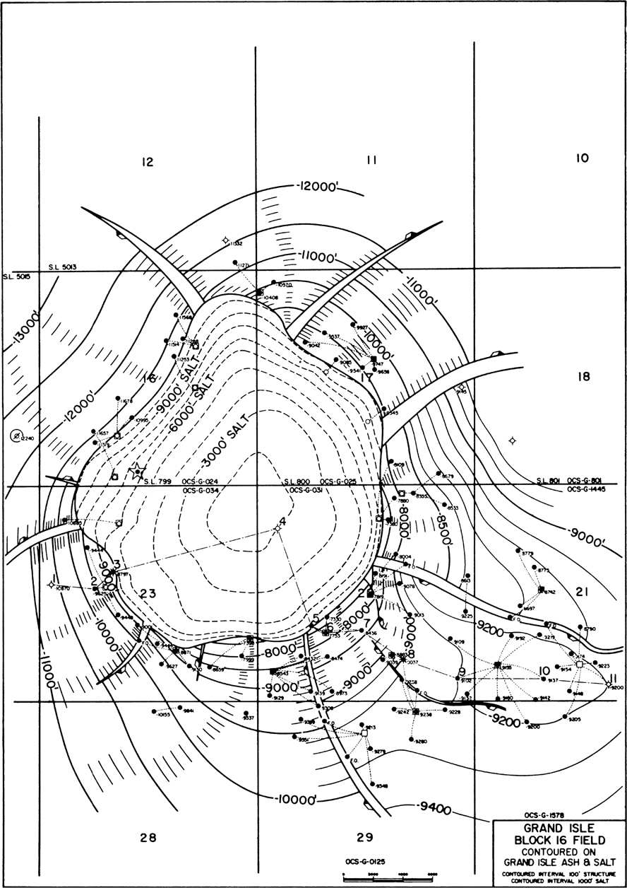
Figure 8-71 Structure contour map on the Grand Isle Ash and on the salt at Grand Isle Block 16 Field, northern Gulf of Mexico. The outline of the salt at this map level is defined by the intersection of the salt and structure contours at the same elevation. (Published by permission of the Lafayette Geological Society.)
As mentioned in Chapter 6, steeply dipping structures, such as those related to salt tectonics, require the layout of a number of cross sections to help develop an accurate geological interpretation and aid in the structure map construction. Typical cross sections for steeply dipping structures such as a salt dome are designed to incorporate both straight and deviated wells. Initially, problem-solving type cross sections are laid out to help resolve correlation problems and aid in developing the structural interpretation. Later, during the advanced stages of mapping, these sections can be converted to finished illustration sections for display and presentation. For further information on the use of cross sections as an aid to structure interpretation and mapping of salt structures, refer to Chapter 6.
A salt diapir commonly forms the core of a large structural high. In response to the draping of strata around the diapir as the structure develops, the strike of the strata is typically parallel or subparallel to the face of the salt. So, the structural contours on a given horizon tend to be parallel or subparallel to contours on the salt surface. This is illustrated in Figure 8-71 for Grand Isle Block 16 Field.
Around certain salt structures, subsurface data show structure contours intersecting salt at a sharp angle. Where this happens, it may be an indication of several possible situations, including (1) the possibility of a salt overhang, such as the one shown in Figure 8-72, or (2) an unrecognized peripheral fault sliding down or located near the face of the salt, causing the strike direction of the contours to appear to turn into the salt. Actually, the contours are striking into the downthrown side of the peripheral fault. Figure 8-73 is an example of such a situation. Notice on the southwestern portion of the salt dome that the contours appear to strike directly into the salt. Due to the complex nature of the faulting pattern, Faults C, D, and E, which appear as radial faults shallow in the section, become peripheral faults with depth, paralleling the southwest flank of this salt structure. As a result, the structure contours tend to strike at various angles into the fault. In contrast, observe the general conformity of the structure contours with the salt on the western and eastern flanks of the structure not affected by peripheral faulting.

Figure 8-72 Generalized cross section of Bethel Dome, Anderson County, Texas, showing a hydrocarbon accumulation below the salt overhang. The significant amount of overhang might indicate that the dome is detached from the salt source bed at depth. (From Salt Domes, by Michel T. Halbouty. Copyright 1979 by Gulf Publishing Company, Houston, Texas. Used with permission. All rights reserved.)
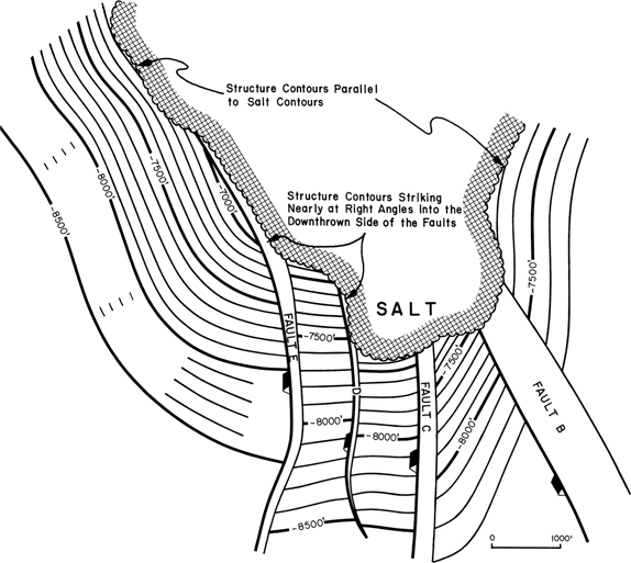
Figure 8-73 Structure contours striking into the downthrown side of Faults E and D give the appearance that the contours are striking into the salt.
Strike-Slip Fault Tectonics
Strike-slip faults are high-angle to vertical faults that form under horizontal compression. A strike-slip fault system may have great linear extent, such as the San Andreas Fault complex, where major lithospheric plates are involved, or it may occur within a local or subregional area as a limited system of finite length. These local strike-slip systems are sometimes referred to as compartmental because of the independent deformation on either side of the fault (Fig. 8-74a). In this type of deformation, a structure that seems to be cut by a strike-slip fault need not have a severed portion offset on the other side of the fault, since the faulting and deformation are contemporaneous and independent on either side of the fault (Fig. 8-74b). In addition to horizontal motion, vertical movement of varying degrees is commonly associated with strike-slip fault systems, as well as fault block rotation. Methods of interpretation and mapping of strike-slip areas are described in Chapter 12.
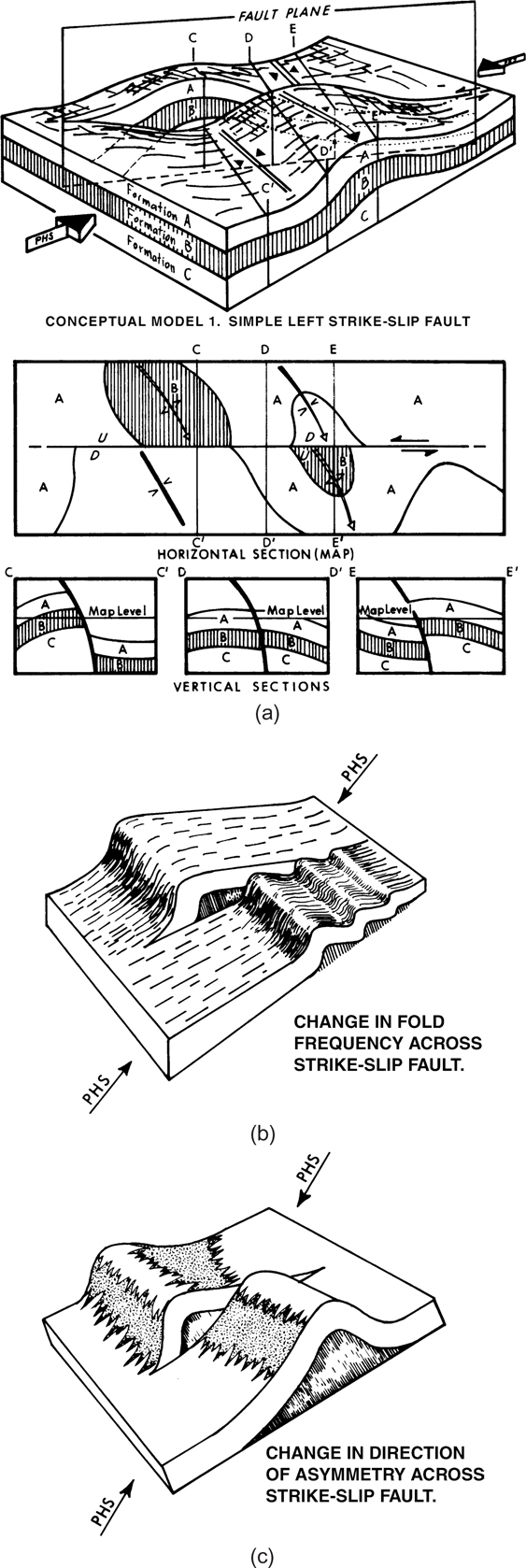
Figure 8-74 (a) Conceptual model of simple left strike-slip fault: Top—block diagram; middle—plan view; bottom—cross-sectional views. (From Stone 1969. Reprinted by permission of the Rocky Mountain Association of Geologists.) (b) Block diagram illustrating different deformational patterns on opposite sides of a finite strike-slip fault. (From Bell 1956. AAPG©1956, reprinted by permission of the AAPG whose permission is required for further use.) (c) The change in direction of asymmetry or fold frequency across the fault is due to a different response to the compressional forces. (From Brown 1982. AAPG©1982, reprinted by permission of the AAPG whose permission is required for further use.)
The primary hydrocarbon traps associated with strike-slip faults are anticlines that straddle the strike-slip system. These anticlines, which may be faulted by either normal or reverse faults, are good traps because they form early and commonly develop large closures sufficient to trap economic quantities of hydrocarbons. In this chapter, our interest is in the mapping techniques that are applicable to these strike-slip fault systems. Figure 8-75 shows an example of a strike-slip fault system with offset faulted anticlines on each side of the fault. In many cases, the faults cutting the anticlines are small and simply offset the structures with little, if any, change in structural attitude across the fault.

Figure 8-75 Typical strike-slip fault system with associated faulted anticlines.
Two different types of mapping techniques are required to map these strike-slip faulted structures. Normally, the structures on either side of the main strike-slip fault must be mapped independently (Fig. 8-75) because structures tend to terminate against the strike-slip fault (Bischke et al. 1990). As for the individual anticlines that form on either side of the main strike-slip fault, the vertical separation technique is commonly applicable for mapping across the faults within these anticlines. In other words, the faulted anticlines commonly exhibit contour (structural) compatibility across the small normal or reverse faults that cut the anticlines, unless some type of rotation occurs along the fault.
Figure 8-76 is a structure map from the Rosecrans Oil Field, California, USA. Evidence from seismic well log correlations and focal mechanism solutions shows that the Newport/Inglewood trend is a transpressional system (Wright 1991) (also consult Figs. 12-12 to 12-14). The Rosecrans Oil Field is one structure along this tread that exists along the western portions of the Los Angeles Basin. Rosecrans Field can be used to illustrate the mapping techniques applicable for a strike-slip fault system. Notice that the anticlines adjacent to the Inglewood Fault are cut by small reverse faults. The cross-section insert and the structure map show that there appears to be structural compatibility across most of these small faults. With the use of well control and seismic data, the vertical separation for each fault can be determined and used to contour across the faults.

Figure 8-76 Rosecrans Field structure (after California Div. Oil & Gas, 1961) shows a distinct pattern of reverse-faulted anticlinal folds oriented obliquely to the Inglewood Fault. (Modified from Harding 1973. AAPG©1973, reprinted by permission of the APPG whose permission is required for further use.)
Notice the two faults labeled C and D on the structure map. Based on this structure map and available cross sections, some fault block rotation, in addition to dip-slip motion, occurred on these faults and resulted in a loss of structural compatibility across the faults. Therefore, it may be difficult, if not impossible, to contour across these faults using the vertical separation. The structures on either side of Faults C (Compton Thrust Fault) and D may require independent contouring. However, north of Fault D the structure again has good contour compatibility across the northern two faults shown on the map. Another possible interpretation for Faults C and D is that these faults do not exist, and instead the apparent faults are actually axial surfaces that bisect kinks in the strata (see Chapter 10).
Figure 8-77 is a structure map on the top of the Ranger Zone in the Wilmington Field in the Los Angeles Basin, California. The anticlinal structure that forms the Wilmington Field is 11 mi long and 3 mi wide. This giant field has produced over 1.2 billion barrels of oil. During the Middle Miocene, compressive stresses formed a north-south couple, folding the strata and establishing the present northwest-southeast Wilmington structure. During its complex structural history, the anticline developed a series of normal faults as a result of tensional forces acting along the structural axis. These normal faults are small, ranging from 100 ft to 400 ft of vertical separation and dipping at angles between 45 deg and 65 deg. Many of the faults are sealing and therefore divide the field into at least seven major production blocks (Mayuga 1970).
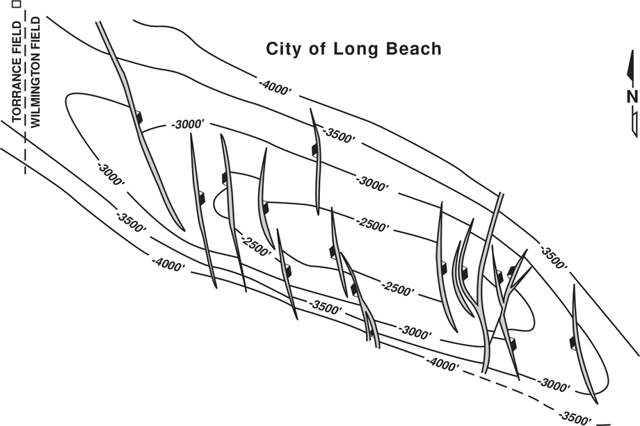
Figure 8-77 Structure contour map on the top of the Ranger Zone, Wilmington Oil Field, southern California. The normal faults in the field exhibit several patterns: (1) single, (2) compensating, (3) bifurcating, and (4) intersecting. Length of the mapped area is about 10 miles. (After Mayuga 1970. AAPG©1970, reprinted by permission of the AAPG whose permission is required for further use.)
A review of the structure map in Figure 8-77 suggests very good structural (contour) compatibility across all the faults in the field. Therefore, all structure and fault map integration in this field would use the vertical separation technique for contouring across the faults. The Wilmington Field is another example of a strike-slip fault-associated structure that exhibits good internal structural compatibility across the faulted anticline.
Compressional Tectonics
Our discussion of compressional tectonic settings includes both high-angle reverse and thrust faults because they commonly occur together in this setting. Also, this section centers on fold-and-thrust belts, which include forearc, backarc, and collisional belts, as they make up the most prolific compressional habitat. The most common hydrocarbon trap is the hanging wall anticline, which includes such structures as fault propagation folds (snakeheads), fault bend folds, and duplex structures (see Chapter 10). For example, in the Wyoming-Utah backarc fold-and-thrust belt fields in the Rocky Mountains, USA (Fig. 8-78), nearly all the hydrocarbons are trapped in the hanging wall of the Absaroka Thrust. They include such fields as Painter Reservoir, Whitney Canyon, Ryckman Creek, and Anschutz Ranch Fields. Nearly all these fields are found in asymmetric anticlinal folds with the steep limb to the east. Collisional zones, such as the Zagros collisional belt of Iran, are some of the most prolific of all fold-and-thrust belt types. At one time, the Zagros belt accounted for 75% of the world’s fold-and-thrust belt production.
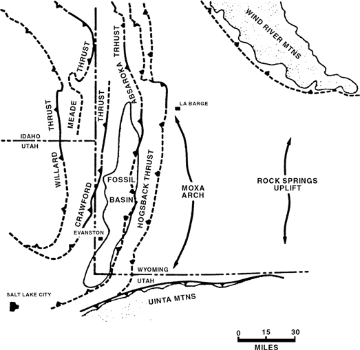
Figure 8-78 Maps showing the position of the Fossil Basin in the hanging wall of the Absaroka Thrust Plate. (From Lamerson 1982. Reprinted by permission of the Rocky Mountain Association of Geologists.)
An extensive literature search yields very few examples of contoured fault surface maps and integrated structure maps for compressional structures. There are volumes of published fault and integrated structure maps for extensional petroleum areas, but they appear to be scarce for compressional areas. The inverse is true for balanced cross sections. A significant number of balanced cross sections have been published for compressional structures, but very few are published in extensional areas.
Fault surface mapping is not commonly done in compressional areas, although there is no reason why it should not be; indeed, the construction of fault surface maps would aid in the understanding of the geology. One possible reason for not making fault surface maps and integrating them with structure maps is that, in many cases, hydrocarbons are trapped in the hanging wall anticline, only slightly disrupted or controlled by reverse or thrust faulting. Therefore, fault surface maps are not prepared. Another reason is that balanced sections are often constructed; therefore, the construction of fault surface maps is assumed unnecessary. We believe, however, that the mapping of all related faults is an essential part of any structural interpretation. In previous sections of this text, we showed that cross sections and seismic sections can misrepresent the actual structure because of the orientation of the line of section. We also mentioned in Chapter 7, with regard to the tying of seismic lines, that any nonvertical event can tie. The test of a valid fault interpretation is the preparation of a fault surface map that is geologically reasonable based on the available data.
We have shown that fault trace construction for any mapped horizon, particularly in areas of steeply dipping beds, cannot be done intuitively. The accurate delineation of a fault trace for any mapped horizon requires the integration of a fault map with the structure map for that horizon. Remember, a fault trace on a specific horizon may be misleading as to the trend and shape of the fault surface itself. The construction of a fault trace on a structure map based on a few well picks and seismic lines is guesswork and is often incorrect. We therefore encourage the construction of fault surface maps in compressional areas.
Reverse Faults.
Earlier in this chapter, we showed the techniques for construction of a reverse-fault surface map and the integration of this map with a structure map (Figs. 8-25 and 8-26). In this section, we look at intersecting reverse faults. Unlike the case involving normal faults, where the fault appears as a horizon discontinuity on the map (a gap), no plan view horizon discontinuity is present on a structure map with a reverse fault. The contours on the upthrown block (hanging wall) overlie the contours on the downthrown block (footwall).
The example in Figure 8-79 is drawn in a form similar to the normal fault examples except that fault transport is reversed to show what happens due to compression. The pattern of intersecting faults illustrates the mapping techniques, but the geometry may not be an accurate predictive model. In other words, reverse faults on a plunging anticlinal structure may result from a volume problem created as planar beds are forced into the compound curvature of the nose. Such faults may not necessarily intersect, because the compression may be accommodated on different stratigraphic levels by separate faults. Intersecting faults do occur in compressional areas, however, and therefore understanding the mapping techniques for these faults is important.
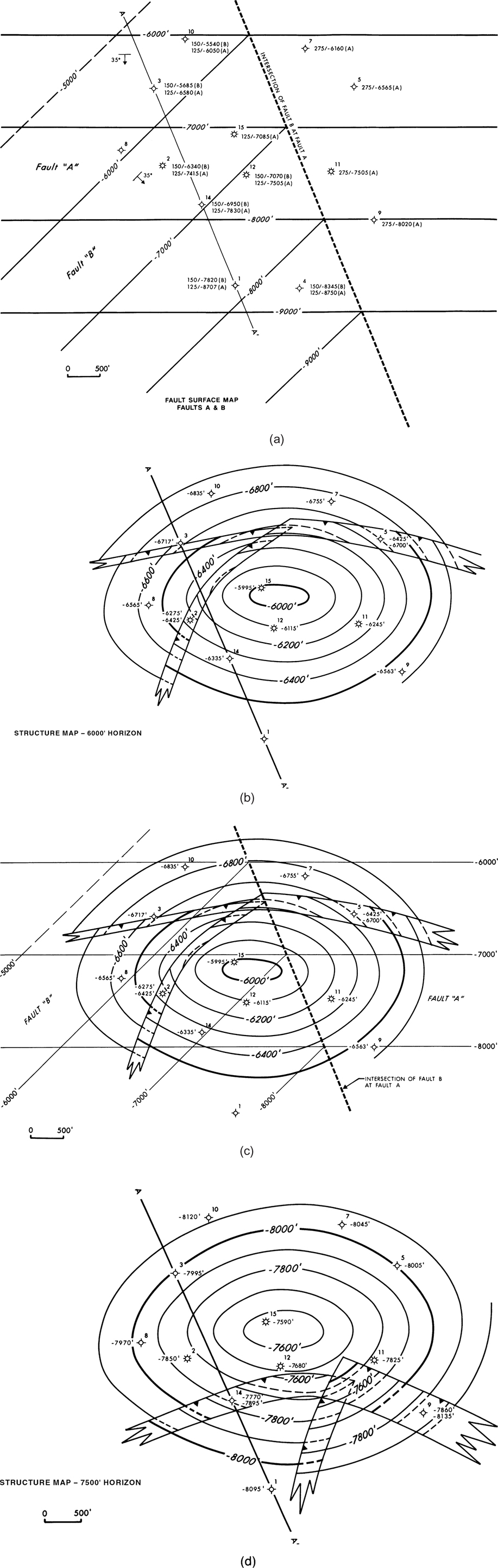
Figure 8-79 (a) Fault surface map for reverse Faults A and B. (b) Integrated structure map on the 6000-ft Horizon. Contours are dashed on the footwall block in the area of fault overlap for clarity. (c) Fault map superimposed onto the structure map to show the accuracy that is achieved by the integration of the two maps regarding: (1) fault trace construction, (2) position of faults, (3) fault intersections, and (4) proper bed contour construction across each fault. (d) Completed structure map on the 7500-ft Horizon. Contours dashed on footwall in area of fault overlap.
Figure 8-79a shows the fault contour map for reverse Faults A and B. Since we are dealing with intersecting faults, the line of intersection must be shown on the fault surface map. Also, the additive property of faults must again be considered; throughout the area where two faults are present (west of the intersection line in our example), Fault A has 125 ft of vertical separation (repeated section in wells) and Fault B has 150 ft of vertical separation. Only Fault A with a vertical separation of 275 ft (150 ft + 125 ft = 275 ft) is present east of the line of intersection. Therefore, the vertical separation is conserved across the line of intersection.
Figure 8-79b is a completed structure map on the 6000-ft Horizon faulted by Faults A and B. Figure 8-79c shows the fault map superimposed on the completed structure map. This figure demonstrates the construction of the upthrown trace (trace on the hanging wall) and downthrown trace (trace on the footwall) for each fault, the construction of the intersection of the traces of the two faults, and the proper bed contour construction across each fault using the vertical separation. We have discussed in detail this type of construction with a number of other examples, so we do not detail the construction here. Instead, we recommend that you pick at least two contours and review the construction techniques used to complete this structure map. Notice that the fault intersections fall on the line of intersection. Figure 8-79d is the completed structure map on the deeper 7500-ft Horizon; take a moment and review its construction. The fault overlaps are wider on this horizon because the faults and the horizon are dipping in the same general direction.
As with normal faults, the construction technique of integrating a fault surface map with a structure map removes all the guesswork with regard to (1) the location of the fault on the mapped horizon, (2) fault trace construction, (3) the location of all fault intersections, and (4) the width of the fault overlaps. The integration of the two maps constructs these features automatically without the need for guesses or estimates.
Thrust Faults.
Most thrust faults have displacements large enough to offset the two fault blocks so that there is no continuity of structure (contour continuity) across the fault. In such cases, each fault block must be contoured independently and then integrated with the fault map or maps.
Figure 8-80a is a diagrammatic cross section of the Mount Tobin Thrust Fault, Nevada. Notice that there has been significant movement of the upper plate over the thrust fault. Therefore, the upper and lower plates of the Ph Bed require independent contouring and fault integration. Figure 8-80b shows the Mount Tobin Thrust Fault map superimposed on the structure map of the top of the Ph Bed in the upper plate. Observe in the upper portion of the figure that the shape of the fault trace on the top of the Ph Bed is shown as a closed oval (in plan view). This type of configuration is not arrived at intuitively; it requires the integration of the fault and structure maps for accurate delineation.
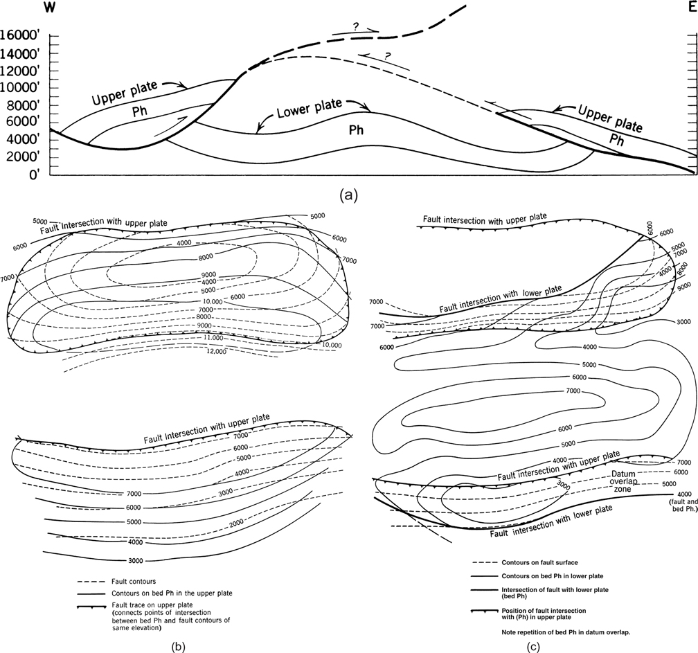
Figure 8-80 (a) Diagrammatic cross section of thrust fault (see Mount Tobin, Nevada, USGS map series GQ7). (Modified from Bishop 1960. Published by permission of author.) (b) Part of upper plate and fault surface map. Delineates the intersection of the fault with the upper plate. (c) Overlay of fault map and lower plate to show the intersection of the fault with the lower plate. (From Bishop 1960. Published by permission of author.)
Figure 8-80c shows the integration of the fault map with the lower plate (the trace on the upper plate is also shown on the map). This example demonstrates the detail required to contour the Ph Bed in the upper and lower plates and integrate these plates with the fault map to accurately determine the position of all the fault traces. Take a few minutes and study the map to be sure you understand how the two maps were integrated to arrive at the finished structure map.
Figure 8-81 is an integrated structure contour map, in two-way time, on the top of the Mirador Formation within the Medina Anticline in the Eastern Cordillera, Colombia (Rowen and Linares 2000). The Medina Anticline was interpreted and mapped based on surface outcrop, well log, and seismic data.
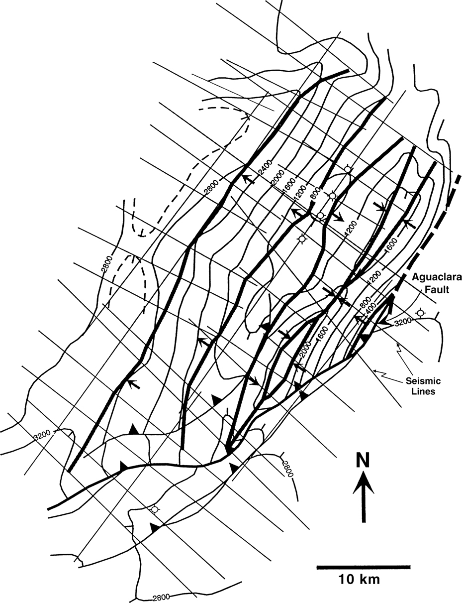
Figure 8-81 Structure contour map of the top Mirador Formation in the Medina Anticline, Eastern Cordillera, Colombia. Thick black lines are axial surface traces interpreted on seismic dip profiles, with arrows pointing in the dip direction. Thick, dashed black line represents erosional truncation at the ground surface. Contour interval is 400 msec, relative to an arbitrary datum near the ground surface. (From Rowan and Linares 2000. AAPG©2000, reprinted by permission of the AAPG whose permission is required for further use.)
The Medina Anticline is an excellent example of the integration of all data sources to (1) generate a fault surface interpretation and map (Fig. 7-34), and (2) integrate the fault surface with the structural interpretation. The Medina Anticline is a fault bend fold in the hanging wall of the Aguaclara Fault in the southeastern thrust belt of the Eastern Cordillera in Colombia. Active exploration in this area of Colombia has resulted in the discovery of several large hydrocarbon accumulations such as Cusiana and Cupiagna. Although the Medina Anticline has well-defined axial surfaces and nearly planar limbs, the fold appears more rounded than kink in shape. In order to complete the interpretation and mapping for prospect generation, the fault surface and structure map should be converted from time to depth.
Finally, remember we discussed the technique of preparing a pull-apart map for compressional areas, or the use of a flap map, when mapping by hand. Such a map allows the contouring of a given horizon all the way to its footwall cutoff, which may be a considerable distance from the leading edge of the hanging wall block. With this technique, the mylar or paper used for mapping is cut along the leading edge of the hanging wall block, and new material is spliced in underneath to allow mapping of the subthrust surface to its fault cutoff. In complex areas with substantial thrust transport, this eliminates the confusion of dashed versus non-dashed contour lines. The maps can be separated to show the whole surface of the mapped horizon in both the upper block and subthrust. They are also very helpful during isochore mapping.
Requirements for a Reasonable Structural Interpretation and Completed Maps
At the end of any interpretation project, the accuracy of the reconstructed subsurface geology depends on the completeness of the work undertaken. We cite 10 requirements that should be met to ensure the best and most accurate subsurface interpretation and final generated maps.
Three-dimensional validity of the interpretation.
A clear understanding of basic geological principles, including the intersecting geometry of horizons and faults.
A good understanding of the tectonic setting being worked.
The use of all the available data.
An understanding of the accuracy of the data.
Correct correlations (well log, seismic, and outcrop where available).
The use of correct and accurate mapping techniques.
The construction and integration of all required maps.
Multiple horizon mapping.
Construction of cross sections (balanced, if possible).
If all these requirements are met, there should be a high degree of confidence that the interpretation and completed maps are reasonable and accurate with respect to the available data.
Multiple Horizon Mapping
Almost any set of fault and structural data can be forced to fit on one particular horizon. The test of the fault and structural interpretation, and whether the interpretation fits on a series of horizons at various depths, lies in structural framework mapping. Therefore, one of the most important of the 10 requirements listed above is the interpretation and preparation of integrated multiple horizon structure maps. Multiple horizon interpretation and mapping means the preparation of structure maps on several horizons to ensure that the interpreted structural framework maintains continuity at all levels. Normally, at least three horizons are required to establish confidence in the interpretation. However, depending on the size of the area being mapped and the number and vertical distribution of pay horizons, additional integrated structure maps at various depths may be required.
Once the structural framework (fault and structure pattern) is established by constructing several fieldwide or regional structure maps at various depths, the mapping of all pay horizons between these initially mapped horizons becomes a much easier task.
Discontinuity of Structure with Depth.
If the structural geology of an area maintains continuity with depth, the mapping of at least three horizons at various depths establishes and supports the structural interpretation. However, in many instances the structural continuity is interrupted with depth by one or more of three primary geological events: (1) unconformities, (2) thrust faults, or (3) listric growth faults. In these cases, the structural geology above the interrupting event most likely will not conform to the structure below. Therefore, separate interpretations are required above and below the interrupting event, in addition to multiple framework horizon mapping.
Figure 8-82 is a cross section through the Painter Reservoir Field in Wyoming. Observe that the structural continuity is interrupted by two different events, first by the Sub-Evanston Unconformity at about 3500 ft, and second at the Absaroka Thrust Fault. Notice how the structure of the area changes above and below each interrupting event. Such major events must be recognized to develop a good structural interpretation and are important in the search for hydrocarbons.
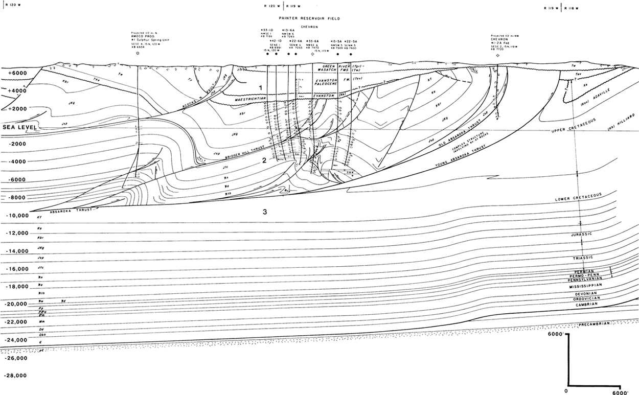
Figure 8-82 Cross section through Painter Reservoir Field. The Sub-Evanston Unconformity and the Absaroka Thrust Fault are interrupting events that result in different structural geometry above and below these events. (From Lamerson 1982. Reprinted by permission of the Rocky Mountain Association of Geologists.)
Perched Water
We have emphasized mapping the top of reservoir beds in this chapter as the structure of the top of the reservoirs controls the trapping of oil and natural gas. It is also important to map the base of the reservoir. A good map on the base of the reservoir is required for accurate volumetric determination of edge water reservoirs, as is discussed in detail in Chapter 14. A base of reservoir map may be necessary for constructing an Allan section, as described in Chapter 4. A base of reservoir map is also helpful in understanding the occurrence and distribution of perched water. Perched water was defined by Gaafar et al. (2016) as “movable water above the transition zone that is not directly connected to the actual free-water table of a given hydrocarbon column.” The perched hydrocarbon/water contact may be a few feet or tens of feet about the field hydrocarbon/water contact, as at Grane Field in the North Sea (Rolfsvag and Danielsen 2016) or hundreds of feet above the field contact as in the 8500-ft Sand in Garden Banks 191 Field (Fugitt et al. 2000) and in the J3 Sand at Holstein Field in the Gulf of Mexico.
Perched water is trapped in closed lows on the base of the reservoir unit. These closed lows could be the irregularities on the base of the reservoir unit in an anticline (Fig. 8-83; see also Figure 5 in Rolfsvag and Danielsen 2016), erosional lows in a stratigraphic trap (Fig. 8-84), or the faulted limb of an anticline (Fig. 8-85). Perched water is in pressure communication with the hydrocarbon accumulation across the hydrocarbon/water contact, but it is not in pressure communication with the regional aquifer (Fig. 8-86).
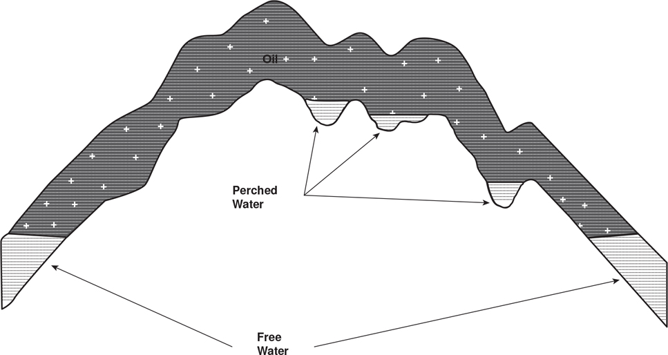
Figure 8-83 Anticline with closed structural lows on the base of the reservoir unit resulting in perched water. (Modified after Weber 1995.)
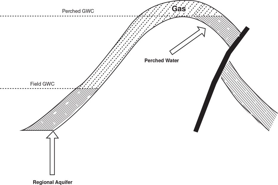
Figure 8-84 Faulted anticline illustrating perched water trapped against a fault. This figure illustrates water trapped against a reverse fault but the figure could just as easily have been drawn with the perched water trapped against a normal fault. (Modified after Weber 1995.)
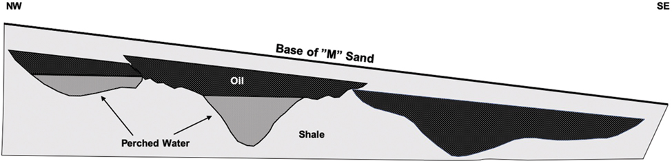
Figure 8-85 Perched water trapped in erosional lows in a system of partially stacked sand bodies inside of a larger erosional scour in the “N” Sand, Ram-Powell Field, Gulf of Mexico. Oil within the individual sands is in pressure communication but the perched water accumulations are isolated from each other. (Modified after Kendrick 2000.)
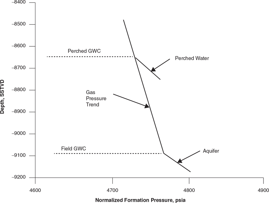
Figure 8-86 Reservoir pressure data from members 3 to 5 of the 8500-ft Sand in four wells in Garden Banks 191 Field in the Gulf of Mexico. One well encountered perched water in this sand. (Modified after Fugitt et al 2000.)
In most cases, the amount of perched water in the reservoir is rather small and does not affect the reservoir volumetrics significantly, although some have suggested that significant impact on volumetrics is possible (Gaafar et al. 2016). As the volume of perched water is relatively small, it does not cone into producing wells. Although the perched water is movable, the compressibility of water is small, and reducing the pressure in the reservoir through production does not cause the perched water to expand appreciably. Because perched water is trapped in structural lows by hydrocarbons, it is isolated from the regional aquifer. If the composition of the regional aquifer changes after the hydrocarbons trap the perched water, the composition of the perched water can differ significantly from that of the aquifer. Perched water may, for example, be highly saline, whereas the regional aquifer salinity may be closer to normal marine salinity. A good structure map on the base of the reservoir should allow the distribution of perched water to be determined, potentially identifying economic volumes of hydrocarbons downdip of the perched water.