Chapter 12. Strike-Slip Faults and Associated Structures*
* For all figures in this chapter (in the printed book only), see the preface for information about registering your copy on the InformIT site for access to the electronic versions in color.
Introduction
Strike-slip displacements occur along near-vertical faults that offset basement (Harding 1990). Displacements along strike-slip faults are predominantly in the strike direction of the fault, and the vertical separations of the horizons along strike-slip faults may alternate between normal and reverse separations. Along active strike-slip faults, dip-slip components of displacement are also common (Clark et al. 1984). As they move, the crustal blocks typically encounter curves or bends in the near-vertical fault surfaces. Material moving into these fault bends may generate structures that can trap hydrocarbons. Commonly, areas may be subject to strike-slip, compressional, and extensional displacements, and the compressional or extensional displacements need not be contemporaneous with the strike-slip faulting (Wright 1991; Shaw and Suppe 1996). This complex style of displacements, combined with the 3D structural development and the progressive nature of the deformation, which changes with time, makes the interpretation of strike-slip faults and their related structures difficult. These complexities often result in the misidentification of strike-slip faults and the misinterpretation of structural styles (Harding 1985, 1990). Strike-slip deformation is truly a four-dimensional problem, which requires an understanding of how the predominantly horizontal displacements occur through time. In this chapter and in Chapter 13, we address the 3D strike-slip problem and propose methods to solve the complexities associated with strike-slip deformation, thus providing ways to improve interpretations used to explore for and develop hydrocarbon resources.
Problems concerning the interpretation of strike-slip faulted structures involve the issue of recognizing empirical evidence for strike-slip faulting (Harding 1985, 1990). According to Harding (1990), “Many workers do not provide evidence for their assertions of strike-slip deformation.” More specifically, some strike-slip interpretations lack direct evidence in support of horizontal displacements. Evidence for horizontal displacements fundamental to strike-slip faulting is critical and, therefore, strike-slip fault interpretations that lack direct evidence for horizontal displacements are questionable. Unfortunately, other structural styles are readily confused with strike-slip styles (Harding 1990), and strike-slip interpretations are often the cause of numerous discussions among working groups. For example, strike-slip interpretations made from poor quality 2D seismic data are often attributed to a different structural style after 3D data are acquired. Once data quality improves, preliminary strike-slip fault interpretations may become (1) inversion structures (Mitra 1993; Link et al. 1996), (2) duplex folding (Mitra 1986; see the Imbricate Structures section in Chapter 10 in this book), (3) growth compressional folding (Suppe et al. 1992; Shaw and Suppe 1994) (Chapter 13), (4) basement structures (Narr and Suppe 1994), or (5) areas of high bed dip. Poor-quality data and an inappropriate structural model can easily result in the misinterpretation of structural style. Our experience suggests that, at times, interpretations may incorporate numerous strike-slip faults into an area that contains minor amounts of strike-slip faulting. We make the case that strike-slip faulting, when viewed in a regional context, is often no more difficult to confirm than other types of faulting. We believe that the releasing bends and restraining bends, common to known strike-slip faults, are fundamental to the understanding and recognition of strike-slip faults and their related structures (Crowell 1974a, 1974b). Their presence is supportive and is often the only direct evidence for strike-slip faults present in subsurface data sets.
In this chapter, we briefly review several misconceptions concerning strike-slip faulting and problems encountered when working with these fault systems. We present methods and techniques for recognizing, restoring, and balancing strike-slip structures. Our goal is to provide the methods with which to generate interpretations and prospects based on observational evidence for lateral displacement, and not on the absence of data. This chapter concentrates on several models and interpretation methods used to interpret strike-slip faulting, and we briefly present the strengths and weaknesses of each model. The manner in which we apply models to geological and geophysical data affect our understanding of the petroleum system and the ultimate success of a prospect or of field development. These models are the stress/strain, surface feature, restoration, releasing bend/restraining bend, and balanced cross-section models. A common theme to this discussion is the application of the standard mapping techniques, methods, and philosophy that we employ when interpreting extensional and compressional regimes. Geoscientists seem best served by establishing 3D structural validity to their interpretations and prospects, as described in Chapters 5, 7, 8, and 9, rather than relying on theoretical models that involve stress or strain. We must get the strike-slip fault geometry correct before embarking on the regional geological model and prospect generation.
All too often, discussions concerning the interpretation of strike-slip faults seem to result in theoretical arguments involving stress or strain. Stress is not commonly measured in subsurface data and are rarely measured in outcrop. Accordingly, the application of stress or strain concepts to prospect generation or regional studies can easily result in disappointment and confusion. For this reason, we begin the discussion of geological models by briefly reviewing the application of stress and strain as applied to prospect generation.
Mapping Strike-Slip Faults
The procedures and methods for recognizing and mapping strike-slip faults are no different from mapping and recognizing other styles of faulting. As discussed in Chapters 1 and 7, the interpretation process starts by constructing viable maps of the large, or structure-forming, fault surfaces. In the interpretation of faults from seismic data, the interpreted profiles are loop-tied in order not to map two faults as a single fault. Viable fault surface maps are typically smooth surfaces devoid of major kinks. Kinks in fault surface maps typically indicate a more complex interpretation, such as the presence of two faults rather than one fault or intersecting faults.
In a typical exploration or development study, after mapping the faults, we integrate chosen horizons into the fault surface maps, as discussed in Chapter 8. We are unaware of any techniques, other than those already discussed in this book, required to integrate strike-slip faults into horizon maps. Thus, if a strike-slip fault exhibits normal separations, then employ the techniques described in the section Techniques for Contouring across Normal Faults in Chapter 8. If a strike-slip fault exhibits reverse separations, then consult the discussion on reverse faults and compressional tectonics in Chapter 8. A discussion of other geometries concerning strike-slip faults and their associated features and styles are in the section on strike-slip faults in Chapter 8 and in the bulk of this chapter.
The Problem of Strike-Slip Fault Interpretation
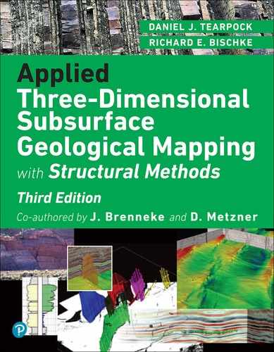
Our review of strike-slip fault interpretations and the associated structures and prospects from around the world suggests that some interpretations of strike-slip faults do not present direct evidence for horizontal displacements. Often, geoscientists do not generate fault surface maps in support of strike-slip faulting. Instead, the working group may rely too heavily on stress/strain models or may interpret strike-slip faults to be within no-data zones on seismic sections. Some of the observed geometries associated with strike-slip faults are inconsistent with simple models of stress or strain (Sylvester 1988). For example, some textbooks on structural geology teach that strike-slip faults are oriented at about a 30-deg to 45-deg angle to the direction of maximum principal stress or strain (the compressional direction), as in Figure 12-1. This simple model of strike-slip faulting assumes a continuous (unfractured), isotropic, and homogeneous body. However, faults and joints introduce discontinuities into rock that invalidate the continuous material body assumption. The crust contains numerous fractures and is not a continuous body (Pollard and Segall 1987). In the following section, we review evidence that this simple model of deformation is inconsistent with the regional orientation and distribution of Neogene fold axes relative to strike-slip faults (Mount and Suppe 1987, 1992).
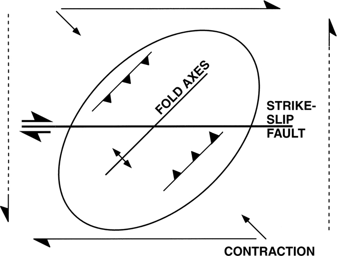
Figure 12-1 Simple model for compression and strain. Strike-slip faults lie at a 45-deg angle, and reverse faults and fold axes form at about a 45-deg angle, from the contraction direction (the direction of maximum principal stress). The simple double-couple model for stress and strain assumes a continuous (unfractured) material body. This model is inconsistent with observed geometrics associated with strike-slip faults.
Strain Ellipse Model
A common model used in prospect generation is one in which strike-slip displacements cause contractional folds to form along and near strike-slip faults. Some structural geology texts teach that these folds form along strike-slip faults according to a simple model of strain, as shown in Figure 12-1. The folds and the throughgoing faults are thought to form as a result of the maximum shear strain oriented parallel to the fault surface. When applying the simple model of strain to strike-slip faults, geoscientists may orient the model so that a shear couple parallels the direction of the throughgoing fault (Fig. 12-1). This assumes a continuous and homogenous medium and that the direction of maximum contractional strain or stress is at a 45-deg angle to the throughgoing fault. However, rock fractures at about a 30-deg angle from the maximum principal stress (Ramsay 1967). Some texts infer from an analysis of the simple shear model that (1) the model accounts for the origin of folds in the vicinity of strike-slip faults, and (2) the model requires the fold axes to trend at high angles (about 30 deg to 45 deg) to the strike-slip faults. This analysis assumes that the plane of maximum shear stress or strain lies near, or in the plane of, the throughgoing strike-slip fault (Fig. 12-1). However, actual folds trend at much lower angles to strike-slip faults (Sylvester 1988), perhaps as a result of rotational displacements.
In the section on balancing strike-slip fault interpretations, we discuss how folds form adjacent to and along strike-slip faults. Folds adjacent to strike-slip faults may or may not exhibit fold axes that trend at 30-deg to 45-deg to the fault surfaces. Figures 12-2, 12-3, and 12-4 show regional Neogene fold axes relative to the San Andreas, Semangko (Indonesia), and Philippine Faults. Notice on the figures that most of the fold axes trend subparallel to the strike-slip fault zones. One would assume that these fold axes lie in a plane that is subnormal to the maximum contraction direction, which in these examples would be subnormal to the surface trace of the strike-slip faults. This orientation of the maximum contraction direction is inconsistent with the simple strain model, and it suggests that the compression subnormal to the faults may be independent of the strike-slip displacements. Furthermore, the neotectonic folds are not concentrated along the fault zones, but rather they exist as far as 50 km to 300 km from the fault zones. Thus, empirical data obtained from areas such as the San Andreas, Semangko, and Philippine Faults do not support the simple model of stress and strain, resulting in the “stress paradox” (Sylvester 1988). The simple theory, if applied to geological or geophysical data, could affect regional and prospect interpretations and your understanding of the petroleum system under study.
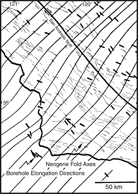
Figure 12-2 Borehole elongations measure the direction of maximum principal stress across the San Andreas Fault, California. Borehole breakout directions (short bold lines), Neogene fold axes (dotted lines), and predicted maximum compressive stress trajectory direction (long thin lines) from breakout data, using a statistical smoothing technique developed by Hanson and Mount, are shown. Maximum compressive stress direction is subnormal to, and Neogene fold axes are subparallel to, the San Andreas Fault. Neogene fold axes extend about 100 km from fault zone. (Published by permission of Van Mount.)
Figure 12-3 Borehole elongations measure the direction of maximum principal stress across the Semangko Fault, Indonesia. Borehole breakout directions rotated 90 deg (short thin lines), Neogene fold axes (dashed lines), and thrust fault earthquake focal mechanism solutions (long thin lines) are shown. Arrows show direction of relative plate motion. Maximum compressive stress direction is subnormal to, and Neogene fold axes are subparallel to, the Semangko Fault. Neogene fold axes extend about 300 km from fault zone. (From Mount and Suppe 1992. Published by permission of the American Geophysical Union.)

Figure 12-4 Borehole elongations are used to measure the direction of maximum principal stress across the Philippine Fault. Borehole breakout directions rotated 90 deg (long thin lines) and Neogene fold axes (rose diagram). Arrows show direction of relative plate motions. Maximum compressive direction is subnormal to, and Neogene fold axes are subparallel to, the Philippine Fault and its branches. Neogene fold axes do not concentrate near the fault zone, but rather extend about 200 km from the fault zone. (From Mount and Suppe 1987 and 1992. Published by permission of Van Mount.)
The fold geometry present on Figures 12-2, 12-3, and 12-4 seems to be in conflict with deductive reasoning concerning continuous material behavior taught in many texts on structural geology. However, some of these observations are consistent with or predicted by more advanced theories on discontinuous material behavior, as presented in texts on strength of materials and rock mechanics.
How are the observations present on Figures 12-2, 12-3, and 12-4 consistent with known principles of mechanics? Displacements along strike-slip faults often create a zone of rubble in the “fault zone.” Broken material is incapable of supporting large stresses or strains (Billings 1972), thus releasing shear strain in the vicinity of the fault zone. The fault gouge also reduces the frictional stress in the fault zone. If the shear strain in the rubble zone approaches zero, then the fault surface lies near a principal plane of stress (Ramsay 1967), and the maximum principal stress could rotate into a position that is subnormal to the fault zone.
Mount and Suppe (1987) propose that the strike-slip motions decouple from the compressional motions, and that plate tectonics may use the transform faults as the “weak link in the chain.” Motion along the weak and low-friction transform faults has the effect of minimizing the work (strain energy) required to drive the global tectonic system. Physics teaches us that the least work solution is the correct solution.
Problems Interpreting Stress
Misconceptions concerning stress can result in incorrect geological interpretations. First, stress is a mathematical and not a physical concept (Jaeger 1962) and is by definition a measure of the intensity of the state of a reaction. Stresses are invisible, so one cannot see a stress; one sees only the results of stress. Alternatively, the force vector is by definition a directed line segment. Forces can be visualized as a load or as a weight. Second, stress is a second-order tensor (Jaeger 1966). The stress tensor exhibits both rotational components and invariant components that are independent of the coordinate system. The tensor components of stress or strain interact with discontinuities to cause the state of stress or strain within a body to be complicated. Rock mechanics textbooks present numerous examples of complicated stress trajectory patterns, related to simple structures, that are certainly not intuitive (e.g., Obert and Duvall 1967). Chinnery (1963) solved the problem of the state of stress along a strike-slip fault using elastic dislocation models. Elastic dislocation models show complicated stress trajectory patterns involving simple structures (Fig. 12-5), particularly at the ends of fractures (Bischke 1974; Xiaohan 1983). The simple model of stress or strain cannot predict the complicated stress patterns associated with faults and fractures.
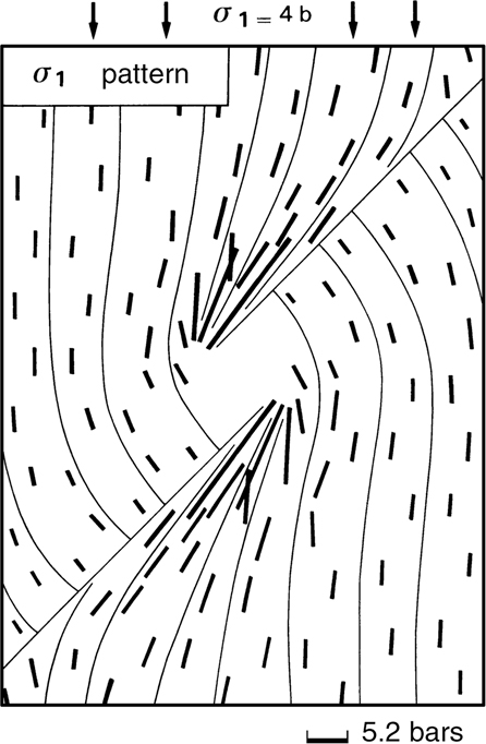
Figure 12-5 Stress trajectories (thin lines) around an en echelon offset, or stepover, in a strike-slip fault. Near the ends of the stepover, the stress trajectories of the maximum principal stresses rotate into the fault as a result of the discontinuity. Stresses are discontinuous across the fault surface and change intensity according to the length of the short bold lines. (From Xiaohan 1983; Guiraud and Seguret 1985. Published by permission of the Society for Sedimentary Geology.)
Geoscientists sometimes attempt to infer the state of stress from geological features or structures. Inferences concerning the state of stress are complicated by several factors, including the rotational property of the stress and strain ellipsoid. As the stress tensor may rotate through time, the finite strain observed in rocks need not result from a unique stress direction (Flinn 1962; Ramsay 1967). Furthermore, geoscientists must measure the state of stress; they cannot directly observe stress. No one has ever seen a stress, certainly not a stress in the distant past. If a structure formed in the distant past, then the stresses that formed the structure may not be recoverable. Thus, we believe that inferences, deductions, and speculations concerning stress often lead to incorrect conclusions concerning structures and prospects. It is not our intent to discuss all the ramifications of stress or strain or their field measurements, which are presented in texts on rock mechanics (e.g., Jaeger 1962; Obert and Duval 1967; Jaeger and Cook 1969). Our point is that speculations concerning stress have little value during the interpretation and prospect-generation process and that these speculations may cause more harm than good. Accordingly, we concentrate on interpretation methods that involve the displacement of stratigraphic units. This approach has an advantage in that displaced horizons are subject to direct observation, as opposed to stresses that are at best measured.
Stress Measurements across Strike-Slip Faults
When attempts were made to measure the stress on the San Andreas (California) and other large strike-slip faults, the results were puzzling (Zoback et al. 1987; Mount and Suppe 1987, 1992). Figures 12-2, 12-3, and 12-4 show the direction of the maximum horizontal stress trajectories, as determined from borehole breakout measurements and earthquake focal mechanisms solutions, for the San Andreas (California), Semangko (Indonesia), and Philippine Faults (Mount and Suppe 1992). The maximum horizontal stress lies in the same plane as the maximum principal stress σ1. These measurements record the state of stress during the Neogene. The borehole breakouts obtained from deep wells react to stresses at depth, below the influence of surface topographic effects. Hydro-fracturing experiments, conducted during enhanced recovery efforts, show that wellbore breakout data record the direction of the minimum principal stress σ3 (Zoback et al. 1985; Zheng et al. 1989; Dart and Swolfs 1992). The direction of maximum principle stress σ1 is 90 deg from the σ3 direction and lies in a plane oriented at right angles to the borehole breakout direction. For three of the world’s major strike-slip faults, stress directions derived from borehole breakout data, as shown on Figures 12-2, 12-3, and 12-4, suggest that the maximum horizontal stress is predominantly subnormal to the strike-slip faults. This is in contrast to the 30-deg to 45-deg angles as predicted by the simple model of stress. This may suggest that major strike-slip faults are low shear stress, or weak, faults. Their fault surfaces apparently lie near a principal plane of stress (Ramsay 1967), where the shear stress, and thus the frictional stress, is low. These stress measurements are consistent with the lack of a heat flow anomaly on the San Andreas Fault (Brune et al. 1969).
From this discussion, we conclude that the simple models of stress and strain are inconsistent with the contractional direction implied by the regional Neotectonic fold axes and borehole breakout directions (Figs. 12-2, 12-3, and 12-4). The simple models of stress and strain do not include material discontinuities in the analysis, so these simple models often fail to predict the trends and the distribution of the observed tectonic features. The fact that the simple theory fails to predict natural features is consistent with advanced theories on discontinuous material behavior and elastic deformation (Pollard and Segall 1987; Obert and Duval 1967). The basic problem of identifying or mapping strike-slip faults is not a mechanical problem, but rather a geometric problem. Perhaps it is time to rethink the strike-slip fault problem, particularly as strike-slip faulting has been difficult to document when interpreting subsurface data.
Applying the appropriate model to describe the stress and strain along fault surfaces is important. Often when confronted with possible strike-slip motions, some geoscientists may model the observed fold axes at about 30-deg to 45-deg angles to the throughgoing strike-slip fault (Fig. 12-1). This approach, which conforms to the assumption of high shear stress, can cause several mapping and interpretation problems. We have seen maps derived from 2D data in which faults and structures were forced to conform to the simple strain assumption shown in Figure 12-1. An incorrect conclusion derived from the application of the simple model may cause several interpretation problems, which are discussed below. It is not our intent to single out specific interpretations, but to improve the understanding of strike-slip structures in order to help geoscientists generate high-quality prospects. Thus, we treat strike-slip faulting as a purely geometric problem that involves standard mapping techniques and methods.
One example of interpretation problems is fitting the simple strain model to nonexistent faults and thereby forcing these nonexistent faults into interpretations. Also, little or no consideration may be given to the exploration potential of structures that exist at a distance from a strike-slip fault. Alternatively, confusion may exist on the part of management as to why the structures do not exist at 30-deg angles to the fault zone, or why structures exist at a distance from the fault zone. Management may assign a higher risk to the area due to these apparent “strange structural complications.”
Geoscientists may believe that folding must have been accompanied by strike-slip faulting in an area under study. Figure 12-1 implies that folds and strike-slip faults exist in common association, which occurs in many areas (Figs. 12-2 and 12-3). However, if strike-slip faults do not exist where folds are present, which is common to many folded terrains, then geoscientists may force strike-slip faults through data in order to satisfy a 30-deg to 45-deg angle assumption. Nonexistent faults may be drawn downward through poor seismic data zones to converge into a deep master basement fault, creating a thick-skinned strike-slip environment, where a thin-skinned compressional environment and hydrocarbon migration model is the appropriate model for the area. The interpretation of an intensely fractured structure may cause management to abandon a good prospect (Tearpock et al. 1994).
In cases concerning en echelon folded structures, interpreters may force strike-slip faults through coherent seismic data that constitute lateral ramps (Chapter 10), or force faults along axial surfaces in an attempt to satisfy the strain ellipse assumption (Fig. 12-1). These practices may result in incorrect seismic correlations, incorrect interpretations and maps, incorrect models of faulting and the petroleum system, and in numerous disappointments and dry holes. This may lead to further confusion concerning strike-slip faulting when evaluating the results of a drilling program and the local petroleum system.
Criteria for Strike-Slip Faulting
How does one recognize that strike-slip displacements exist in an area? Harding (1985, 1990) discusses seismic criteria for the recognition of strike-slip faults. His checklist includes the first three of the following main criteria, to which we add two other important and definitive criteria recognizable in petroleum-related data sets. We also provide additional criteria that directly follow from Harding’s analysis.
During strike-slip faulting, a large, near-vertical master fault offsets basement and cover rocks (Harding 1990). In many cases, magnetic deconvolution can help resolve the depth to magnetic basement (Hartman et al. 1971). These relationships are shown on Figure 12-6 near sp 820 where a near-vertical branch of the Philippine Fault displaces magnetic basement and cover rocks (Bischke et al. 1990). The fault cannot rotate into a vertical position as a result of imbricate faulting.
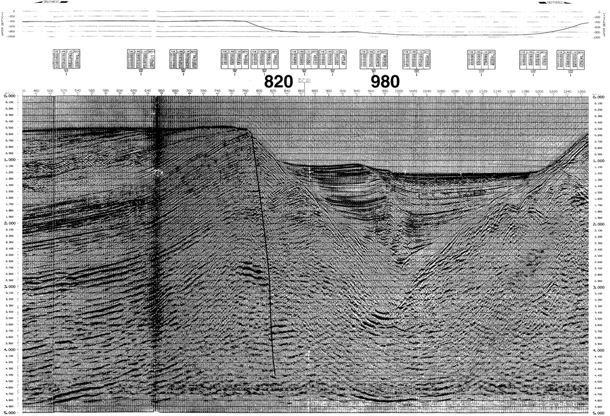
Figure 12-6 A large branch of the Philippine Fault, projected in from subsurface data and nearby surface maps from the island of Masbate. Large fault offsets magnetic basement represented by the bold reflections at sp 820 at 2.70 sec. The fault surface is nearly vertical. A minor splay images near sp 980, where the seismic stratigraphy and bed dips change across the fault surface. (From Bischke et al. 1990. Published by permission of the Philippine National Oil Company.)
The seismic stratigraphy of the sediments on the opposite sides of the near-vertical fault should be fundamentally different (Harding 1990) (Fig. 12-6 at sp 980). The juxtaposed seismic stratigraphy should be shown as not resulting from inversion structure or growth reverse faulting (see Chapter 13).
The structure and seismic reflections are discontinuous across a high-angle fault surface (Harding 1990) (Fig. 12-6 at sp 980). If you can easily correlate the seismic reflection character and geology across a possible strike-slip fault, then strike-slip faulting is probably not present. In this case other types of faulting should be considered.
Fault surface maps depict a steeply dipping, high-angle surface (Shaw et al. 1994) that may contain en echelon offsets, or stepovers (Aydin and Nur 1982). Fault surface mapping introduces 3D structural validity into interpretations. Surprisingly, in the literature we have seen no viable map of a fault surface, generated from seismic profiles, presented in support of strike-slip faulting. Figure 12-18 is a map of a restraining bend on the San Andreas Fault based on aftershock activity rather than on seismic or well data.
The en echelon offsets are the sites of the compressional restraining bends and the extensional releasing bends, such as the rhombochasms and tipped wedge basins (Crowell 1974a, 1974b). These bends are recognizable on fault surface maps constructed along strike-slip faults, where they appear as bends in the fault surface. Criteria 4 and 5 are discussed in detail in the following sections.
If the preceding criteria are met within an area, then the application of a strike-slip fault model is warranted (Harding 1990) but not proven. Across normal and reverse faults, the hanging wall and footwall cutoffs of correlatable beds record the sense and the amount of the vertical and horizontal separations. If the cutoffs are recognized, then vertical and horizontal displacements are proven. However, across strike-slip faults, commonly no cutoffs exist to record the horizontal separations along straight-line segments of strike-slip faults. Unfortunately, 2D fault patterns or sets of divergent or convergent fault patterns, as interpreted on seismic profiles, do not provide direct evidence for lateral displacements. These divergent or convergent fault patterns provide evidence for vertical separations, but not actual horizontal displacements. Thus, strike-slip faulting requires a 3D analysis in support of horizontal displacements. The problem with these criteria, which are suggestive of strike-slip faulting, is the inability to directly address the issue of horizontal displacements. Economics obligates geoscientists to present viable interpretations rather than concepts “drawn on a seismic background,” as Bally (1983) correctly recognized.
Analysis of Lateral Displacements
In this section, we review a number of geological features used to document horizontal and vertical displacements on strike-slip faults. Documenting vertical displacements is important in the extensional releasing bends and the compressional restraining bends (Crowell 1974a, 1974b). We place particular emphasis on the local and regional restoration of geological features. These methods are capable of documenting the amount of lateral displacements, which are important when projecting sand trends or when analyzing the petroleum system. We begin with a discussion of surface geological features.
Surface Features
A number of surface features exist in association with strike-slip faults that support lateral or horizontal displacements in the Holocene. These geomorphic features include sag ponds, shutter ridges and pressure ridges (Allen 1962), offset river channels (Wallace 1968), and surface fractures (Wallace 1973). Topographic and geological maps present evidence of Holocene strike-slip motions.
Piercing Point or Piercing Line Evidence
Piercing point or piercing line evidence involves the displacement of geological features that were initially intact, or unbroken, prior to faulting. A piercing line can be some linear feature that is offset by faulting, and each offset end of the piercing line is a piercing point. Piercing points can also represent a nonlinear feature offset by faulting. These reference features can be seen in outcrop, imaged on a seismic profile, or constructed within a map or cross section.
Pregrowth strata, which are intact prior to faulting, constitute the best piercing line evidence. In growth strata, if stratigraphic intervals correlate across the structure or fault surface, then these syntectonic strata can provide good piercing line evidence. In this case, the sedimentation rate exceeds the tectonic uplift or fault slip rate. If, however, the fault slip rate temporarily exceeds the sedimentation rate, then the syntectonic sediments may contain an initial offset across the fault surface. Alternatively, reconstructions based on sediments deposited in a starved basin environment will contain a displacement error commensurate with the size of the initial offset. If the strata correlate across the fault surfaces, then these errors are likely to be small.
Faults displace distinctive stratigraphic horizons, diapirs, dike swarms, mountain ranges or basins. If one of these features is cut by a fault, then the feature may be restorable to its initial position. To determine the approximate slip on a fault, simply move the strata back along the fault until the displaced feature restores to its approximate initial, or intact, position (Sylvester 1988). The feature restores back to its initial configuration at a corresponding piercing point or line. For example, if a normal fault displaces a horizon, then the hanging wall cutoff restores back into its corresponding footwall cutoff. A 2D seismic profile would intersect the hanging wall and footwall cutoffs at two points. If the profile aligns in the direction of fault slip, then the structure restores back to its corresponding piercing points.
Some features provide better piercing point evidence than others. For example, stratigraphic pinchouts or subcrops provide better piercing point evidence than isopach or isochore maps constructed from syntectonic sedimentary intervals. The stratigraphic pinchout or subcrop information represents a “line in space,” whereas an isopach map represents thickness information. Thus, problems concerning thickness changes related to syntectonic sedimentation often arise where the stratigraphic units change thickness across active fault surfaces. Stratigraphic thickness changes can result from a variety of causes, such as growth faulting and its associated syntectonic sedimentation, or from paleotopographic slopes that cause changes in basin configuration and environments. Geoscientists have documented growth sedimentation across all known geological structural styles, including compressional features and strike-slip faults (see Chapter 13).
Isopach or isochore information, if based on pregrowth strata that change stratigraphic thickness, provides good piercing point evidence. A discussion of methods for distinguishing between pregrowth and growth strata are in Chapter 13.
Other features that represent good piercing point evidence include offset zoned diapirs, mountain ranges, volcanic belts, and basins. Zoned diapirs and basins contain walls and flanks that represent offset surfaces where faulted. These features are useful for recognizing strike-slip faulting if the contacts are nearly vertical and correlatable. Mountain ranges and volcanic belts contain structures and trends that may be restorable, although mountain ranges and basins could contain pre-existing offsets such as the salients and en echelon folds common to fold-thrust belts. Offsets along salients and en echelon folds can be large and can introduce large errors into reconstructions. Subsequent fault motion may occur along these potentially weak, pre-existing offsets.
We discuss two types of piercing point evidence: first, the less definitive regional restoration process, then, the more definitive local and balanced restoration process.
Regional Restoration.
Geoscientists use regional features to determine the approximate amount of slip along strike-slip faults. The Great Glen Fault in Scotland displaced a zoned granite batholith an apparent distance of 65 miles (105 km) (Kennedy 1946). In California, the San Andreas Fault offsets rocks to the north of the Salton Sea and those flanking the Soledad Basin by 250 km (Crowell 1962). The Garlock Fault apparently displaces a Mesozoic dike swarm and other geological features over a horizontal distance of 65 km (Fig. 12-7). The Philippine Fault system offsets Oligocene-Miocene intermediate and siliceous igneous rocks, ophiolite belts, and the intervening Central Luzon Valley-Llocos Basins up to 200 km to 300 km (Fig. 12-8). Gravity, isopach, and isochron maps can be subject to similar regional restoration.
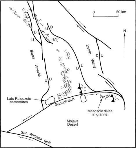
Figure 12-7 Offset features along Garlock Fault, California (Suppe 1985).
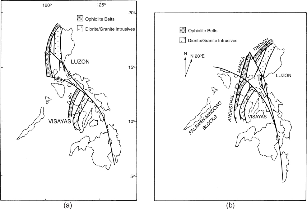
Figure 12-8 (a)–(b) Restoration of Philippine Fault, using long-wavelength features such as ophiolite belts, sedimentary basins, and volcanic chains. (From Bischke et al. 1990. Published by permission of Tectonophysics.)
Regional restorations of long-wavelength features such as volcanic chains and mountain belts, gravity and magnetic anomalies, unconformity intersections, and isopach thicknesses provide insight into the approximate amount of horizontal slip on strike-slip faults. These approximate restorations, in support of strike-slip motion, are more convincing when supported by the criteria discussed in the section on criteria for strike-slip faulting.
Local Restoration.
Commonly, the best available evidence in support of strike-slip faulting is the presence of the ubiquitous restraining bends and releasing bends (Crowell 1974a, 1974b). Restraining and releasing bends document horizontal displacements, and the restoration of these features, using piercing point and piercing line evidence, can determine the approximate slip along fault surfaces (Hill and Dibblee 1953).
The known strike-slip faults of the world are not perfectly straight faults, but contain small to large en echelon offsets, called stepovers, that form restraining and releasing bends (Aydin and Nur 1985) (Fig. 12-9). Table 12-1, taken from Aydin and Nur (1982), lists constraining and releasing bends from various areas of the world.
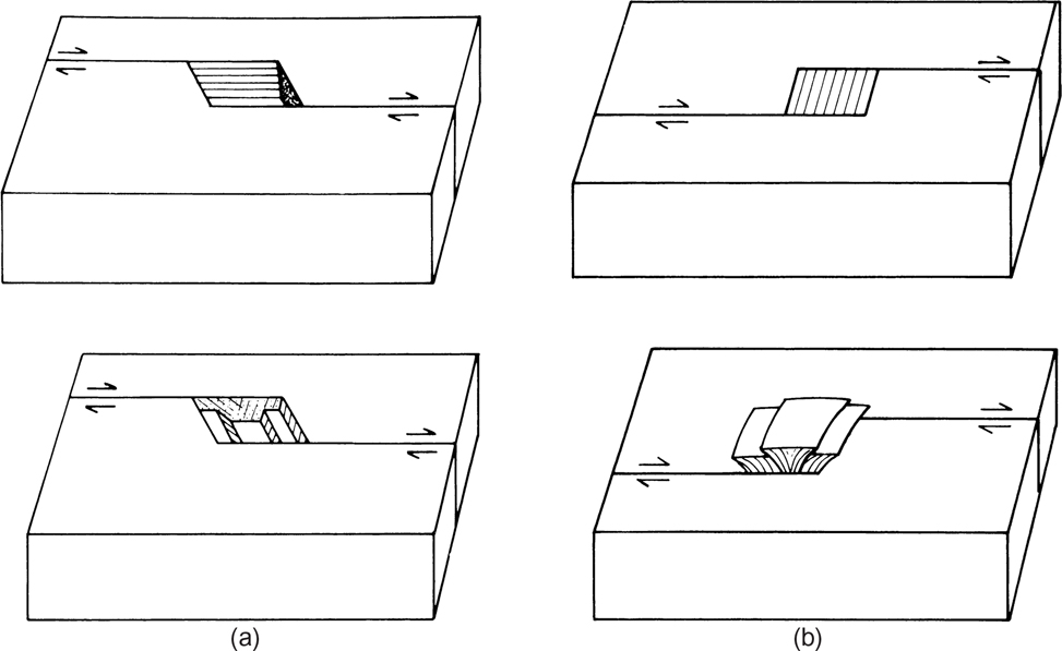
Figure 12-9 (a)–(b) Geometry of releasing and restraining bends (Aydin and Nur 1985). (a) If material moves away from a stepover, then extension and resultant normal faults develop a releasing bend. Structural lows exist in the area of the stepover. (b) If material moves into a stepover, then compression and resultant reverse and thrust faults develop a restraining bend. Structural highs exist in the area of the stepover. (From Aydin and Nur 1985. Published by permission of the Society for Sedimentary Geology.)
Table 12-1 Size of restraining and releasing bends along strike-slip faults. (Aydin and Nur 1982. Published by permission of the American Geophysical Union.)
Fault and/or Location |
Basin or Mountain Range |
Graben (G) or Horst (H) |
Dimension (M) |
Reference |
|
|---|---|---|---|---|---|
Length |
Width |
||||
Motagua, Guatemala |
Motagua Valley |
G |
50,000 |
20,000 |
Schwartz et al. [1979] |
Rio El Tambor |
G |
25 |
8 |
||
Polochic |
Lago de Izabal |
G |
80,000 |
30,000 |
Bonis et al. [1970]; Plafker [1976]; this study |
Dead Sea Rift, Israel |
Hula |
G |
20,000 |
7,000 |
Freund et al. [1968] |
Lake Kineret |
G |
17,000 |
5,000 |
||
Ayun |
G |
6,600 |
1,600 |
||
East of Timna |
G |
1,000 |
250 |
||
North of Ayun |
G |
1,200 |
400 |
Garfunkel et al. [1982] |
|
G |
1,200 |
400 |
|||
G |
1,600 |
450 |
|||
G |
5,000 |
1,200 |
|||
G |
2,000 |
500 |
|||
South of Timna |
G |
8,800 |
3,000 |
||
G |
20,000 |
6,000 |
|||
West of the Dead Sea |
G |
3,500 |
750 |
Garfunkel [1982] |
|
G |
3,000 |
750 |
|||
G |
3,000 |
800 |
|||
G |
6,000 |
1,500 |
|||
G |
7,500 |
1,800 |
|||
G |
3,000 |
750 |
|||
East of the Dead Sea |
G |
4,500 |
1,500 |
||
Paran |
Karkom |
G |
18,000 |
6,000 |
Bartov [1979] |
G |
6,000 |
1,500 |
|||
Bir Zrir, Sinai |
G |
5,000 |
2,000 |
Eyal et al. [1980] |
|
Gulf of Elat |
Elat |
G |
45,000 |
10,000 |
Ben-Avraham et al. [1979] |
Aragonese |
G |
40,000 |
9,000 |
||
Tiran-Dakor |
G |
65,000 |
8,000 |
||
Dasht-e Bayaz, Iran |
G |
1,200 |
500 |
Freund [1974] |
|
Hope, New Zealand |
Medway-Karaka |
G |
700 |
230 |
Freund [1971] |
Glynnwye |
G |
980 |
210 |
||
Glynnwye Lake |
G |
1,800 |
550 |
||
Polars Station |
G |
2,300 |
900 |
||
Hanmer Plains |
G |
13,000 |
3,500 |
Freund [1974] |
|
Hope, New Zealand |
Medway-Karaka |
H |
90 |
30 |
Freund [1971] |
Glynnwye Lake |
H |
300 |
90 |
||
Poplars Station |
H |
300 |
150 |
||
Hanmer Plains |
H |
4,500 |
2,700 |
||
North Anatolian, Turkey |
Niksar |
G |
25,000 |
10,000 |
Seymen [1975]; this study |
Erzincan |
G |
40,000 |
12,000 |
Ketin [1969] |
|
Susehri |
G |
23,000 |
6,000 |
||
San Andreas, California, USA |
Cholame Valley |
G |
17,000 |
3,000 |
Jennings [1959]; Brown [1970] |
San Bernardino Mountains |
H |
32,000 |
14,000 |
Dibblee [1975] |
|
Imperial |
Brawley |
G |
10,000 |
7,000 |
Johnson and Hadley [1976]; Sharp [1976, 1977] |
Elsinore |
Elsinore Lake |
G |
12,000 |
3,000 |
Rogers [1965] |
Garlock |
Koehn lake |
G |
40,000 |
11,000 |
Jennings et al. [1969]; |
G |
300 |
150 |
Smith [1964]; Clark [1973]; this study |
||
G |
600 |
110 |
|||
West of Quail Mountain |
G |
600 |
100 |
||
G |
240 |
90 |
Clark [1973] |
||
G |
900 |
220 |
|||
Searleys Valley |
G |
1,600 |
380 |
||
East of Christmas Canyon |
1,250 |
250 |
|||
San Jacinto, |
Hog Lake |
G |
680 |
170 |
Sharp [1972] |
Hemet |
G |
22,000 |
5,000 |
Sharp [1975] |
|
Buck Ridge |
Santa Rosa Mountain |
G |
6,000 |
1,700 |
Sharp [1972] |
Coyote Creek |
Ocotillo Badlands |
H |
5,500 |
1,800 |
Sharp and Clark [1972] |
Borrega Mountain |
H |
4,000 |
1,600 |
||
Bailey's Well |
G |
500 |
200 |
Clark [1972] |
|
G |
190 |
80 |
|||
Olinghouse, Nevada |
Tracy-Clark Station |
G |
70 |
40 |
Sanders and Slemmons [1979]; this study |
G |
160 |
90 |
|||
G |
450 |
175 |
|||
G |
980 |
250 |
|||
Bocono, Venezuela |
La Gonzales |
G |
23,000 |
6,200 |
Schubert [1980a] |
Merida-Mucuchies |
G |
6,200 |
1,700 |
Schubert [1980b] |
|
G |
700 |
200 |
|||
G |
280 |
70 |
|||
Valencia |
Lake Valencia |
G |
30,000 |
11,500 |
Schubert and Laredo [1979] |
El Pilar |
Casanay |
H |
3,000 |
1,200 |
Schubert [1979] |
Alternatively, restraining and releasing bends form at bends in strike-slip fault surfaces (Crowell 1982). If slip along the linked strike-slip fault system moves material away from the stepover or bend in a fault surface, then the resulting extension forms releasing bends (Fig. 12-9a). If, however, slip along the stepover or bend moves material into the stepover or bend in the fault surface, then the resulting compression causes restraining bends (Fig. 12-9b) (Crowell 1974a, 1974b; McClay and Bonora 2001).
Releasing Bends.
If motion at a stepover or bend in a strike-slip fault creates extension, then a basin bounded by normal faults develops (Fig. 12-9a and b). Two examples of this type of motion are segments of the Hope Fault, New Zealand, and the San Jacinto Fault, California, USA (Suppe 1985) (Fig. 12-10b and c). The San Jacinto Fault is part of the San Andreas Fault system.
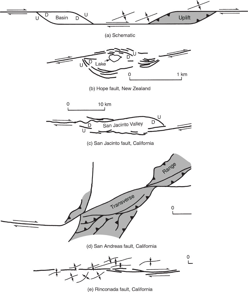
Figure 12-10 (a)–(e) Examples of releasing and restraining bends (Suppe 1985).
Releasing bends form as material within a stepover is subjected to extension. The amount of extension is related to the amount of slip on the strike-slip fault system. According to the releasing bend model, strike-slip faults bound the basin on two parallel sides and normal faults bound the basin on the other two sides. The strike-slip faults form the walls of the basin between the stepover, and normal faults form basin margins at the ends of the stepover (Fig. 12-9a). As the basin extends, material slumps into the void created by the extension parallel to the direction of strike-slip fault motion, and thus the extension records the amount of displacement that formed the basin. To determine the approximate amount of motion that formed the bend, restore the bend by moving the correlatable strata back in a direction that is opposite to the direction of strike-slip displacements.
If the subsidence rate in the basin exceeds the sedimentation rate, then the syntectonic sediments deposited concurrent with strike-slip displacements may contain initial offsets across the normal fault surfaces. Although releasing bends provide direct evidence for horizontal displacements, the restoration of releasing bends may overstate the amount of the strike-slip displacements, if the upthrown block does not contain growth sediments. Sequence stratigraphic evidence, based on high-stand or low-stand evidence, can minimize the amount of error encountered during the restoration process. However, if the stratigraphy easily correlates across fault surfaces, then any error in restoration is likely to be small.
The normal faults that form the margins of the basin contain hanging wall and footwall cutoffs that form piercing lines (Fig. 12-11a and b). These piercing lines represent the hanging wall and footwall cutoffs mapped in three dimensions. The piercing lines form as the blocks at the edge of the extensional basin slump into the basin subnormal to the surface trace of the strike-slip fault. Thus, if we can assume that the direction of strike-slip motion is parallel to the surface trace of the strike-slip fault (i.e., in the strike direction of the mapped fault surface), then we can restore, or close, the basin by moving the strata in the opposite direction of fault displacements and along any number of profiles that parallel the surface trace of the strike-slip fault (Fig. 12-11b and c). The hanging wall cutoffs restore back into the footwall cutoffs at their corresponding piercing points located along the piercing line (Fig. 12-11c).
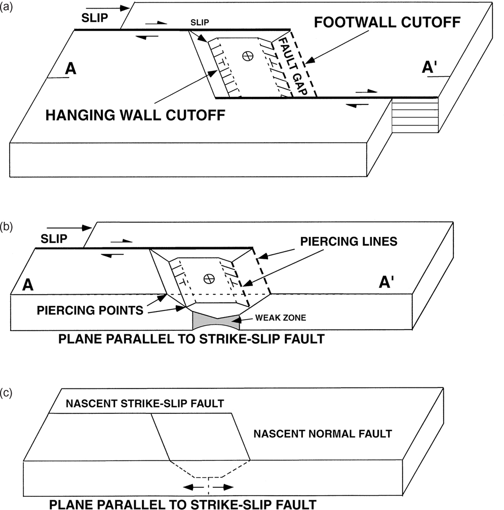
Figure 12-11 Motion along a strike-slip fault can be restored by (a) mapping the hanging wall and footwall cutoffs. (b) A profile taken parallel to the surface trace of the strike-slip fault cuts the piercing lines, creating piercing points. (c) The piercing points are restored back to an undeformed position. (Published by permission of R. Bischke.)
Restraining Bends.
If material moves into a stepover or bend, compression occurs in the restraining bend (Crowell 1974a, 1974b; Aydin and Nur 1985; Cunningham and Mann 2007). The compression forms reverse faults, thrust faults, and pressure ridges, or pop-ups (Fig. 12-9b). A description of the complex deformation occurring on a pop-up from 3D seismic data is in Durand-Riard et al. (2013). This example is on a clear restraining bend. McClay and Bonora (2001) present several examples of restraining stepovers from Nevada, Wyoming, Chile, and the Netherlands. The Transverse Ranges of California, which exist on the Great Bend, a stepover in the San Andreas Fault, are an example of a large restraining bend (Fig. 12-10d). Contraction also occurs at restraining bends on continuously curved strike-slip fault surfaces. Modern 3D seismic time seismic data image these offset bends (Benesh et al. 2014). We discuss an example along the Loma Prieta bend in the San Andreas Fault in a later section in this chapter.
Let’s restore a small restraining bend to illustrate how the process confirms the presence of strike-slip displacements, restores the initial Pliocene stratigraphic trends, and allows us to estimate the amount of Pliocene displacements. This knowledge will allow interpreters to converge on the geometry and history of the Pliocene structures and the associated petroleum system. The bend is located on the flank of the Long Beach Anticline in the Newport-Inglewood Trend, southern California, USA. The Newport-Inglewood Trend is a classic zone of “transpressional” deformation (Harding 1973). The strike-slip faults along the trend form left-stepping, en echelon offsets, and the Cherry Hill and Northeast Flank Faults are major faults in the Newport-Inglewood Trend. Along the southern flank of the Long Beach Anticline, the Northeast Flank Fault steps over to the Cherry Hill Fault (Wright 1991) (Fig. 12-12a). Trenching indicates that the Cherry Hill Fault dies out to the southeast of the map area. Motion along the Newport-Inglewood Trend is right-lateral and, therefore, the bend should be subject to compression. If we assume that material enters the bend parallel to the surface trace of the Northeast Flank Fault or the Cherry Hill Fault, then the resulting contraction is restorable. This contraction forms the Signal Hill Promontory, or pressure ridge (Fig. 12-12b), and a reverse fault that dips at about 50 deg to the southeast (Taylor 1973) (Fig. 12-13). The method of implied fault strike (Tearpock et al. 1994), when applied to Taylor’s map of the bend in the Northeast Flank Fault (Fig. 12-12a), shows that the fault strikes about N65E beneath Signal Hill. The reverse fault motions cause the hanging wall beds and footwall beds to form piercing lines that strike northeast-southwest beneath Signal Hill.
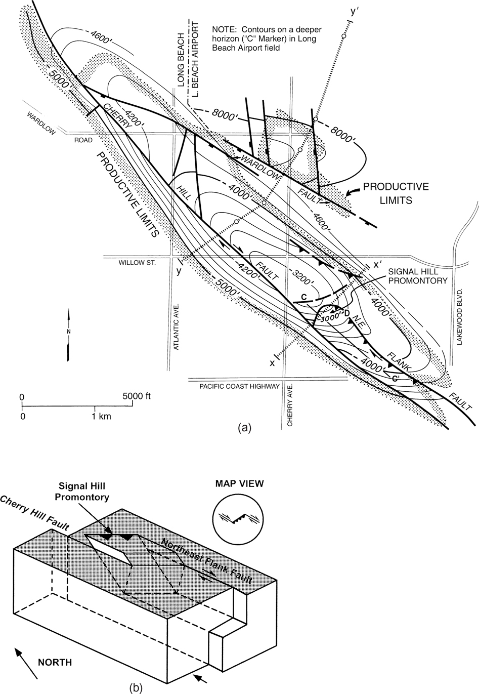
Figure 12-12 (a) Structural map of Long Beach Anticline showing Cherry Hill and Northeast Flank faults that locally define the Newport-Inglewood Trend. Profile C-C′, which trends NW-SE across the Signal Hill pressure ridge, is parallel to the surface trace of the Northeast Flank and Cherry Hill Faults. (Modified from Wright 1991. AAPG©1991, reprinted by permission of the AAPG whose permission is required for further use). (b) Structural model for Signal Hill restraining bend. Northeast Flank Fault bends to the southwest linking to Cherry Hill fault, forming a restraining bend. (Published by permission of J. Shaw and R. Bischke.)
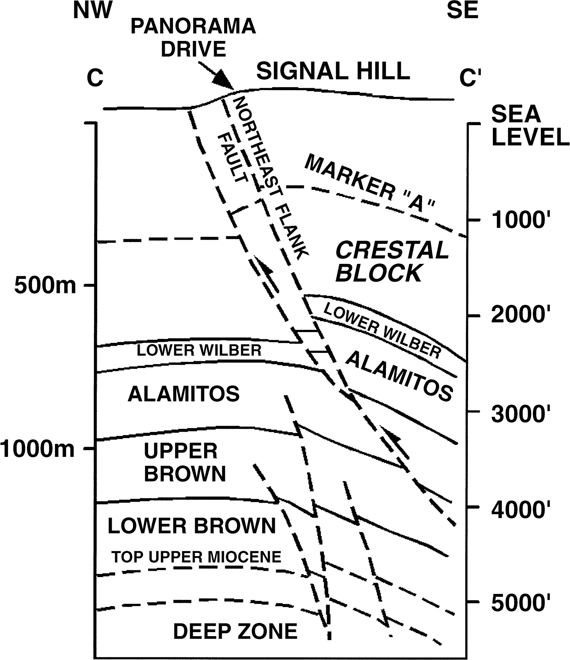
Figure 12-13 Cross section C-C′ across Signal Hill, parallel to Cherry Hill Fault. See Figure 12-12a for location. (Redrawn after Taylor 1973.)
Some textbooks seem to imply that strike-slip and compressional displacements are causatively related, and that transpressional strike-slip displacements commonly generate compressional folds adjacent to strike-slip faults (Fig. 12-1). The Signal Hill pressure ridge formed on the flank of the Long Beach Anticline, but strike-slip displacements need not be the cause of the Long Beach Anticline itself (Wright 1991). In this case, a decoupling of the strike-slip displacements from the compressional displacements may be more appropriate.
Several empirical observations support a decoupling process, which could change the interpretation of the Newport-Inglewood Trend. For example, according to the transpressional explanation shown in Figure 12-1, the axis of the folds would initiate at 30-deg to 45-deg angles to the strike-slip fault. The strains required to rotate a fold axis through a 30-deg to 45-deg angle suggest large amounts of strike-slip displacements. As the axis of the Long Beach Anticline is parallel to the Cherry Hill Fault (Fig. 12-12a), the strike-slip displacement on the Cherry Hill Fault should be substantial. Harding (1973) makes the observation that fold axes are presently offset only by 200 m to 800 m, but some or most of this displacement could be an initial offset of the axes of compartmentalized folds (Chapter 8, Fig. 8-74). The front limb of the Long Beach Anticline is not offset from its crest (Wright 1991) (Figs. 12-13 and 12-14). A second observation is that the structural contours in the hanging wall of the Northeast Flank Fault (Fig. 12-12a) are compatible with the footwall structural contours. This structural compatibility also implies small Plio-Pleistocene displacements (see Chapter 8). Thus, some or all of the displacements on the Northeast Flank Fault appear to be younger than the Long Beach Anticline, which supports Wright’s (1991) observations that the Newport-Inglewood Trend exhibits a complex structural and stratigraphic history not easily reconciled with a simple strike-slip origin.

Figure 12-14 Restored Signal Hill block that was thrust to the northwest. Block restores by moving strata back along the Northeast Flank Fault parallel to the surface trace of the Cherry Hill and Northeast Flank Faults. Restoration shows a pre-existing Long Beach folded anticline. (Published by permission of R. Bischke.)
If you construct a fault surface map for the Northeast Flank Fault along the southeastern flank of the Long Beach Anticline, it shows that the fault surface curves beneath Signal Hill (Taylor 1973), where the fault strikes at about N65E (Fig. 12-12). To the southeast of the anticline, the fault dips at high angles and strikes at about N60W (Fig. 12-12). A seismic or geological profile, such as cross section C-C′ taken in the NW-SE direction (and across the curved portion of the fault surface), will confirm whether the beds are thrust, reverse, or normally faulted. In this case they are reverse faulted (Fig. 12-13) and, referring to Figure 12-9, we can deduce the correct sense of strike-slip motion. That confirms the Signal Hill restraining bend to be a small but obvious restraining bend.
It is obvious from this discussion that in order to locate bends in fault surfaces, it is necessary to construct accurate maps of the fault surfaces, as described in Chapter 7. Typically, a 2D seismic grid is sufficient for constructing general fault surface maps and permits the detection of gentle bends in fault surfaces. Bends or offsets in fault surfaces have important consequences concerning the correct interpretation of data, prospect generation, or the absence of prospects (Tearpock et al. 1994). This is another reason for constructing loop-tied fault surface maps. As curved fault surfaces create releasing and restraining bends along strike-slip faults, maps of these fault surfaces may readily solve difficult structure problems.
The Signal Hill restraining bend is restorable along any number of profiles aligned subparallel to the surface trace of the Cherry Hill or Northeast Flank Faults (Figs. 12-13 and 12-14). The Northeast Flank Fault exhibits about 150 m of vertical separation and about 170 m of horizontal separation in the Pliocene Lower Wilber and Alamitos horizons. These displacements are in general agreement with Harding’s (1973) estimates. The Northeast Flank Fault cuts the southeastern limb of a pre-existing Long Beach anticline (Figs. 12-12 and 12-14) and appears younger than the compressional folding that formed the Long Beach anticline. The strike-slip motion may decouple from the compressional motions that formed the Long Beach Anticline (Shaw and Suppe 1996). Therefore, the compressional and strike-slip motions may not be directly related.
A misconception concerning piercing points is that offset fold axes, once thought to represent a continuous line, are good piercing point evidence because these offset fold axes restore to a single line. However, fold compartmentalization caused by tear faults are known to exist (Chapter 8, Fig. 8-74), and associated folds may form with an initial offset, and not along a single unbroken fold axis. These initial offsets can be large. In addition, folds forming along tear faults may grow during the deformation process, contributing to the offset. Unfortunately, we find that most types of piercing point evidence are rare or absent from most subsurface data sets.
In summary, the releasing and restraining bends, which are common to the known strike-slip faults throughout the world, often provide the best evidence in support of strike-slip faulting (Aydin and Nur 1985). If you are working a suspected strike-slip fault, locate a bend to confirm the strike-slip motions. Partially linked strike-slip fault systems typically contain stepovers. Often, a quick look at a structure map containing a strike-slip fault interpretation can resolve the presence or absence of strike-slip faulting in a matter of minutes. If strike-slip faults are thought to be in the area, examine a structure map for the presence of en echelon stepovers. Next, inquire as to the direction of fault motion. If fault motion moves material into the bend, then a structural high should exist on the map in the area of the restraining bend (Figs. 12-9b and 12-12). If, however, fault motion moves material out of the bend, then a low should exist on the map in the area of the releasing bend (Figs. 12-9a and 12-10b and c). An exception to this quick-look technique is structural inversion, which can also produce high and low areas along en echelon inversion faults. If a regional strike-slip fault interpretation does not contain restraining and releasing bends, perhaps style of faulting is present.
The documentation of strike-slip motion may be no more difficult than the documentation of other types of fault motion, but specific technical work must be done. First, fault surface maps, constructed in support of the deformation, should contain geometries that are consistent with the highs and lows on horizon structure maps. Second, in other tectonic regimes, whether it be compressional, extensional, or salt-related deformation, geoscientists and management require direct evidence of the type and style of the deformation. Strike-slip faults are not two-dimensional, and thus they require a 3D analysis. In many cases, the answer lies in a 4D analysis of the problem (Wright 1991). We presented techniques that can rapidly resolve the interpretation of strike-slip faulting that are no more difficult than techniques required to confirm other types of faulting. These techniques are supported by empirical evidence that establishes 3D structural validity.
Modern explorationists place emphasis on the petroleum system and its associated risk factors. To better understand how structures form and how faulting affects structural development and hydrocarbon migration, a good understanding of fault timing and geometry is necessary. We know of no way to address these issues concerning risk without fault surface maps, correctly interpreted from loop-tied data. If fault surface maps do not exist, then interpreters working an area have imprecise knowledge as to how the local structures formed and how the recognized faults may have channeled hydrocarbons. How can geoscientists correctly identify and understand the type and style of faulting, and generate viable prospects, without constructing viable maps based on loop-tied data? Furthermore, these maps of the fault surfaces may contain subtle bends that indicate small restraining and releasing curves, thus generating additional prospective structures. Fault surface maps also may record the strike-slip motions, as we show in a following section.
If accurate fault surface maps are not available, then it is possible to misidentify the structural style. On 2D seismic data, one may factor flower structure fault geometries (Harding 1985) into the risk analysis, where in reality inversion is the correct structural style. The petroleum system model may erroneously contain thick-skinned vertical faults, whereas in reality the faults are thin-skinned, low-angle faults. This can have a major effect on the interpretation of how hydrocarbons migrate and enter structures. Thus, differences in structural style can impact the understanding of the petroleum system, the interpretation model, the determination of risk, and the ultimate success of an exploration or development program.
Strike-slip faulting is sometimes over-interpreted and confused with other structural styles (Harding 1985), and some interpretations may lack positive evidence in support of horizontal displacements. Too often, strike-slip fault interpretation and the related structures are supported by a lack of data, no-seismic-data zones, high bed dips, axial surfaces, misapplied seismic interpretation rules, and so on (Tearpock et al. 1994). Certainly, strike-slip faulting should be subject to the same scientific methods and subsurface mapping standards that apply to other styles of faulting. Your success as a geoscientist depends on high-quality interpretations, maps, and prospects. Only solid scientific work, as described here, can ensure the best chance of success.
Scaling Factors for Strike-Slip Displacements
Scaling laws for faults allow us to predict the approximate length of all faults, including strike-slip faults. These empirical laws can keep interpretations focused and accurate in order to improve the success rate for finding hydrocarbons. Aydin and Nur (1982, 1985) conducted two interesting studies of restraining and releasing bends and developed a scaling law for the length of strike-slip fault bends. Their study has implications regarding the development of strike-slip faults that may not be totally understood. Aydin and Nur investigated 11 major strike-slip faults in various areas around the world, and they measured the length and the width of 70 restraining and releasing bends associated with those faults (Table 12-1). The width of bends was not independent of the length of bends, as one would assume from the model shown in Figure 12-15. Instead, the lengths (L) of bends are proportional to the widths (W) by the relation
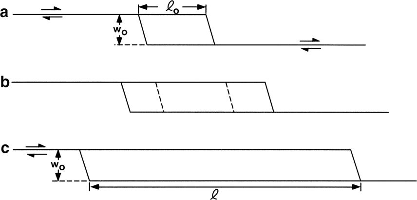
Figure 12-15 A simple model of a strike-slip fault that has a releasing bend that grows in length as the slip on the fault increases. According to this model, the width (w) of the bend should be independent of the length (l) of the bend. Strike-slip faults do not behave according to this simple model, and real strike-slip faults exhibit a relationship in which length is proportional to width. (From Aydin and Nur 1982. Published by permission of the American Geophysical Union.)
Equation 12.1 indicates that L is approximately equal to 3.2 W, at the 95% confidence level. The formula implies that the widths of bends widen as the slip on the faults increases. This implies that smaller bends may coalesce and cluster into larger bends (Aydin and Nur 1982), or that fault zones grow wider as the faults grow in length.
The consequences of their study are multifold. Strike-slip bend widths can be used to estimate the lengths of bends. Large strike-slip faults have wide bends (Fig. 12-10d), whereas small strike-slip faults have narrow bends. It is possible, however, that a large strike-slip fault may deactivate and a new fault may replace a major fault, which would start the process over again. As large strike-slip faults have wide bends, these wide bends should be easy to locate during a regional analysis, and help to confirm the strike-slip interpretation. Narrow bends on small strike-slip faults may be more difficult to locate. In this case, however, the strike-slip process is less important and other processes may dominate, such as extensional or compressional faulting or folding.
We know of no well-documented example by which large amplitude anticlines, domes, structural highs, or basins form as a result of small amounts of strike-slip motion. If the amount of strike-slip deformation is small, the exploration emphasis must shift from processes associated with strike-slip faulting to processes associated with other types of faulting. Another consequence of the study of releasing and restraining bends is that the bends are relatively common along strike-slip faults (Table 12-1). Lastly, as releasing bends grow wider with increasing slip, smaller basins that form within each bend may widen to form larger basins.
Balancing Strike-Slip Faults
The subject of balancing strike-slip faults is in its infancy. We have heard arguments to the effect that large amounts of displacement along some strike-slip faults preclude any attempt to balance or restore the displacements. In the Local Restoration section, we show that large strike-slip faults are locally restorable at their restraining and releasing bends. The concept of piercing lines or points enables geoscientists to restore the section under the assumption that material either enters or leaves the bend parallel to the surface trace of the strike-slip fault. Similarly, in the Regional Restoration section, long-wavelength restorations of major geological or geophysical features document the amount of strike-slip displacements on several well-known faults. Geoscientists have made considerable progress in restoring and documenting (Durand-Riard et al. 2013) strike-slip deformation in three dimensions.
Compressional restraining bends balance if we use the methods outlined in the section on compressional faulting in Chapter 10. We can balance extensional releasing bends using the methods described for extensional faulting in Chapter 11.
Compressional Folding along Strike-Slip Faults
Surface geological information allows us to generate a balanced cross section that is comparable to the subsurface geometry along a portion of the San Andreas Fault in California, as defined by earthquake hypocenters. The Loma Prieta Earthquake occurred on a restraining bend of the San Andreas Fault (Shaw et al. 1994; Schwartz et al. 1994) (Fig. 12-16). In the Loma Prieta epicentral zone, the surface of the San Andreas Fault changes its strike from N40W (320 deg) to N50W (310 deg) (Fig. 12-17). Material entering this restraining bend should therefore be subject to compressional as well as strike-slip motions. Accordingly, the focal mechanism solution for the earthquake inferred from first-motion studies is oblique-reverse, right-lateral motion (Oppenheimer 1990). Geodetic data indicate 1.6 m ± 0.3 m of strike-slip and 1.2 m ± 0.3 m of reverse slip during the earthquake (Lisowski et al. 1990). A fault surface map derived from aftershock hypocentral locations is shown in Figure 12-18a. The fault surface changes strike and dip along its trend. The curved shape of the fault surface, as defined by the hypocentral data, generates a restraining bend. Other strike-slip faults should exhibit similar geometries (Durand-Riard et al. 2013; Benesh et al. 2014).
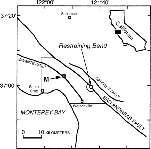
Figure 12-16 Location map of Loma Prieta earthquake and restraining bend on San Andreas Fault, with 1989 earthquake epicenter at M. (From Shaw et al. 1994, United States Geological Survey Publication.)

Figure 12-17 Geological map of Loma Prieta epicentral area showing Glenwood syncline emanating from bend in surface trace of San Andreas Fault. Balanced cross section B-B' is shown in Figure 12-19. San Andreas Fault turns from 320 deg to 310 deg, forming a restraining bend. (From Shaw et al. 1994, United States Geological Survey Publication.)

Figure 12-18 (a) Fault surface map for Loma Prieta restraining bend showing locations of cross sections 1, 2, and 3. (b) Cross sections of San Andreas Fault as defined by hypocentral activity. The fault bends at cross section 2 at a depth of 8 km and it dips at a higher angle at cross section 3. (From Shaw et al. 1994.)
Before entering the bend, the Pacific Plate moves in the N40W (320 deg) direction parallel to the surface trace of the San Andreas Fault. As material enters the bend to the north of Watsonville/Freedom (Fig. 12-17), the Pacific Plate moves up the ramp formed by the southwesterly dipping, high-angle reverse-strike-slip fault surface (Fig. 12-18a). The upward motion generates compressional synclines, similar to synclines that form at the base of compressional thrust fault ramps (Chapter 10). In this example, the syncline should emanate from where the fault surface bends and departs from its general N40W (320 deg) trend. In the south, hypocentral solutions define a San Andreas Fault that dips at 82 deg and strikes N40W (320 deg) (Profile 3 of Fig. 12-18b). In the restraining bend and at Profile 2 of Figure 12-18b, the fault changes in dip to 65-70 deg at 8 km depth and strikes at N50W (310 deg). As predicted, material entering this bend in the fault surface generates the Glenwood syncline (Fig. 12-17). This syncline terminates at the southern bend in the fault surface, northeast of the Rapp Well, where the San Andreas Fault departs from its general N40W (320 deg) trend (Fig. 12-17). Ground-surface dip data present on the surface geological map and well log data constrain the geometry of the Glenwood Syncline (Figs. 12-17 and 12-19).
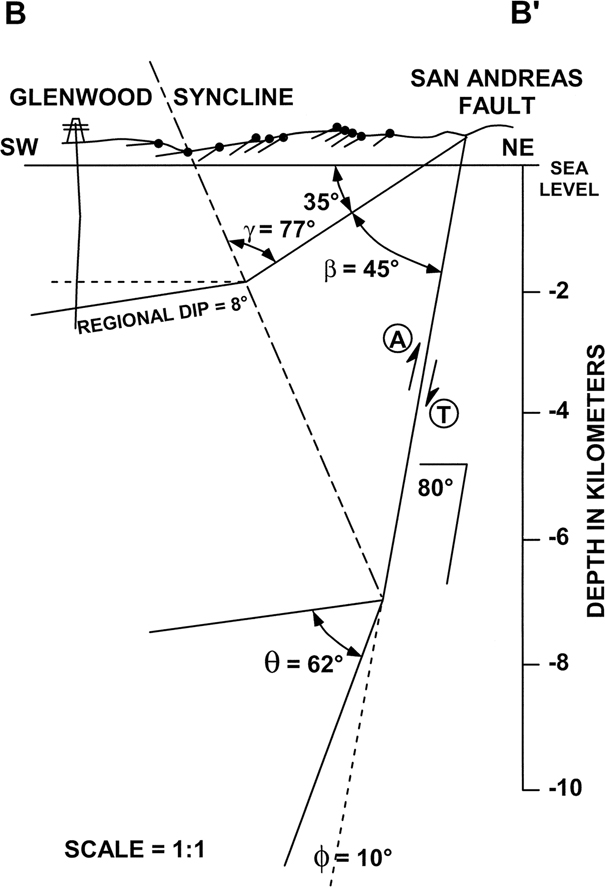
Figure 12-19 Example of a balanced strike-slip fault model for the Loma Prieta restraining bend, San Andreas Fault, California, simplified from Shaw et al. (1994). Model uses ground-surface bed dip data, well control, and dip of San Andreas Fault at the ground surface. The model contains a fault bend at 7 km, in good agreement with hypocentral data along the fault during the Loma Prieta Earthquake. See Figure 12-17 for location.
In the brittle regime of the earth’s crust, folds form as hanging wall beds move over nonplanar fault surfaces (Bally et al. 1966; Suppe 1983). Thus, we can use surface and well data related to the Glenwood Syncline to generate balanced models of strike-slip compressional folding along the San Andreas Fault. Cross section balancing allows us to predict the subsurface fault geometry from the surface and well data. In practice, this exercise allows geoscientists to predict the vertical and lateral dimensions of the hanging wall geometry (Tearpock et al. 1994). Hanging wall geometry is important in positioning wells, in understanding the size of a prospect, and in generating admissible interpretations of strike-slip faults (see the generic example in this section). We use the balanced model to predict subsurface fault geometry and compare the model predictions against the observed fault surface geometry as defined by hypocentral earthquake activity.
Sometimes fault surfaces image on seismic data sets, but the hanging wall structure does not clearly image. Balancing techniques can predict fold shape from fault shape (Tearpock et al. 1994; Shaw et al. 1994) and help constrain interpretations. We balance profile B-B′ on Figure 12-17 (profile 2 in Fig. 12-18b) and present it as Figure 12-19. One of two approaches can be employed in order to balance a profile. If the subsurface fault geometry is known from depth-corrected seismic sections and well control or, in this case, hypocentral aftershock activity, then geoscientists can generate a balanced, or generic, model of the hanging wall structure. Alternatively, if the shallow hanging wall geometry variables γ and β are known from depth-corrected seismic sections, outcrop data, or well control, then geoscientists can estimate the fault surface geometry variables θ and ϕ (Fig. 12-19), where
γ = angle between synclinal axial surface and the adjacent strata
β = angle between shallower portion of strike-slip fault and bedding
θ = angle between deeper portion of strike-slip fault and bedding
ϕ = difference in dip angle between shallower and deeper portion of strike-slip fault
In this case, we use surface dip data and shallow well control to determine γ, the angle between the axial surface and the adjacent beds of the Glenwood Syncline (Fig. 12-19). The hanging wall cutoff angle β, in Figure 12-19, can be determined from local bed dips and fault geometry. By definition,
The flank of the Glenwood Syncline adjacent to the fault dips at an average of 35 deg to the southwest (Figs. 12-17 and 12-19), whereas regional dip is 8 deg southwest in the area west of the synclinal axis. Well log and surface dip data from along the trend of the Glenwood Syncline constrain the regional dip. Thus, to determine β, subtract the dip of the flank of the Glenwood Syncline from the observed surface dip of the San Andreas Fault within the restraining bend. The surface dip of the fault is about 80 deg (Brabb 1989), and thus β = 80 deg − 35 deg = 45 deg. From inspection of Figure 12-19, the axial surface angle γ can be determined from the kink law (Chapter 10), or from the following equation.
Therefore,
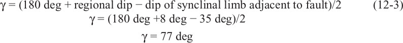
Dip data at the ground surface is used to position the axial surface (Fig. 12-19). The axial surface is drawn downward at an angle of 69 deg (77 deg − 8 deg) until it reaches the fault. This point determines the position of the bend in the fault. Horizons on the synclinal limbs can now be constructed, with the fold hinge bisected by the axial surface.
We next consult the fault-bend fold graph (Fig. 10-38) to generate a balanced solution to the fault surface problem. The correct graph to use is the diagram for synclines (right graph). The values required are γ = 77 deg, recorded on the y-axis of the graph, and β = 45 deg. The values for β are recorded by the right-sloping bold diagonal lines. Project a horizontal line into the graph from the value of γ = 77 deg. Where the γ = 77 deg line intersects the β = 45 deg curve, the change in fault dip angle ϕ is read off the graph from the thin, near-horizontal and downward-sloping curve on the graph. The value of ϕ is slightly less than 10 deg.
Therefore, we conclude that the Glenwood Syncline is created by about a 10-deg subsurface bend in the San Andreas Fault. The axial surface of the Glenwood Syncline emanates from this subsurface bend in the San Andreas Fault, where the previously undeformed beds moved over the bend in the fault surface (Fig. 12-19). As described previously, the depth to the bend in the fault surface was determined by projecting the axial surface of the Glenwood Syncline downward to where it intersects the 80-deg dipping fault. The axial surface intersects the San Andreas fault at a depth of about 7 km (Fig. 12-19). Below this depth, the fault takes a 10-deg bend and the balanced model predicts a fault dip of about 70 deg below 7 km (Fig. 12-19).
We can now compare the model-generated values and the predicted depth of the fault bend to profile 2 in Figure 12-18b. The strike-slip fault bend fold model predicts that the San Andreas Fault makes about a 10-deg angle bend at a depth of about 7 km and that the fault dips at about 70 deg below 7 km (Fig. 12-19). These values compare favorably with the hypocentral data that suggests about a 10-deg fault bend at a depth of about 8 km. Below this depth, the fault dips at about 70 deg, as shown in Figure 12-18b, Profile 2. Given the good agreement between theory and observation, strike-slip fault bend fold theory may allow geoscientists to make viable predictions of the structural geometry along strike-slip faults (Shaw et al. 1994). Balanced cross sections of compartmentalized displacements along strike-slip faults may help geoscientists generate higher quality prospects in a tectonic environment that has proven to be difficult to quantify. When millions of dollars are at stake, deterministic models may add value to conceptual interpretations of prospects generated in strike-slip faulted tectonic regimes.
The San Andreas Fault is subject to hundreds of kilometers of slip, which created the Glenwood Syncline with a broad south-dipping limb (Fig. 12-17). This limb could form a three-way closure against the San Andreas Fault. Other strike-slip faults that contain smaller amounts of slip should succumb to an analysis similar to what we have presented here. Balanced solutions of these structures can improve prospect viability, perhaps solve complex structural problems, and thereby reduce prospect risk.
Generic Example of Strike-Slip Compressional Folding.
If fault surface maps are obtainable from well log or seismic data, then balanced models of hanging wall geometries are possible. Balanced models of hanging wall geometries lead to viable, low-risk prospects. A generic example is shown in the cross section presented in Figure 12-20. Perhaps your working group was subject to the following type of problem that employed well log and seismic data. Let us assume that two companies find hydrocarbons in Wells No. 2 and 3, in the A, B, and C Horizons adjacent to a vertical fault. Outcrop and seismic data suggest that the near-vertical fault, containing restraining and releasing bends, is located between Wells No. 1 and 2 (Fig. 12-20). The two companies construct cross sections of the new field in order to propose additional development wells. In Figure 12-20, well log data constrain the fault geometry, but what is the limit of the field, and is it necessary to drill additional wells?

Figure 12-20 Well log data along a known strike-slip fault. The seismic data as collected are incoherent between dashed lines. Structural data are not subject to unique interpretations, which can result in dramatically different solutions to well-constrained seismic and well log data. (Published by permission of R. Bischke.)
We consider two interpretations of the data: a qualitative interpretation presented by Company A and a quantitative interpretation presented by Company B. We discuss the Company A interpretation first. We make the assumption that geoscientists from Company A do not have a solid background in structural geology and therefore have not been trained in volume conservation or structural balancing concepts. They construct a cross section through the field that employs conceptual, but not volume, conservation concepts. On the other hand, geoscientists from Company B construct a balanced cross section of the existing data. How may these two working groups and their interpretations differ? Can the difference affect future exploration and success? We will assume that the 3D seismic data that crosses the area is of reasonable quality but suffers from the usual problems, such as surface statics and the inability to image steeply dipping beds.
After examining the data present in Figure 12-20, the Company A geoscientist interprets a secondary fault along the western flank of the structure. Two independent sources of evidence exist for this fault. The first piece of evidence is the no-data seismic zone on the flank of the structure (Fig. 12-20). The second piece of evidence is the change in thickness of the stratigraphic units above the D Horizon, between Well No. 2 and Well No. 3. The interpretation is shown in Figure 12-21. The proposed secondary fault exhibits normal, strike-slip, and reverse separations, and it explains the bed dip and thickness variations between the B and C Horizons and the C and D Horizons in Wells No. 2 and 3. This fault geometry also accounts for the slip reversal between the B and D Horizons. Strike-slip faults can exhibit normal, reverse, and lateral separations. The interpreted fault turns down and merges with the large, master strike-slip fault at depth.

Figure 12-21 Company A geoscientists solve the folded-structure problem by using the concept of a secondary fault, related to strike-slip displacements, to explain the apparently high bed dips and vertical thickness changes interpreted from the wells. They propose two additional wells to test the A and B Horizons. (Published by permission of R. Bischke.)
Lastly, Company A completes the seismic interpretation by correlating the reflections from the crest of structure into the off-structure flank position located to the west of the no-data zone on the seismic data set. In the low dip area to the west of the no-data zone, the seismic images a gently folded structure in which the reflectors turn up beneath the secondary fault (Fig. 12-21). The turned-up beds are interpreted to be caused by fault drag on the secondary fault, as is shown in many structural geology textbooks (Billings 1972).
The Company A team present the cross section of the folded and faulted structure shown in Figure 12-21. Using cross sections and maps of the field, they propose two additional wells to define the western limits of the field. These wells will test the upturned A and B Horizons located beneath the fault.
The Company A interpretation makes three basic assumptions: first, that the no-data zone on the seismic data set results from faulting; second, that faulting causes changes in thickness of stratigraphic intervals as seen in well logs, perhaps associated with repeated or missing section; third, that folds tend to be gently curved, rounded features, as shown in some textbooks on structural-metamorphic geology (see Chapter 10). Does another interpretation of the data exist that applies to the low temperature portions of mobile belts?
The Company B geoscientist team, having knowledge of structural geology concepts and techniques, attempts to balance the data shown in Figure 12-20 using procedures developed in Chapter 10 and in this chapter. They notice that the D Horizon is on the same structural level in Wells No. 2 and 3, and thus this horizon is not subject to possible faulting or folding between these two wells. Procedures outlined in the section on compressional folding along strike-slip faults suggest that the D Horizon may be near a bend in the vertical fault. Using the fault cuts located below the D Horizon in Wells No. 2 and 3, the Company B geoscience team reasons that the cutoff angle (θ) between the D Horizon and the deeper part of the fault is 60 deg (Fig. 12-22). Thus, the difference (ϕ) in dip angle of the fault is 30 deg.
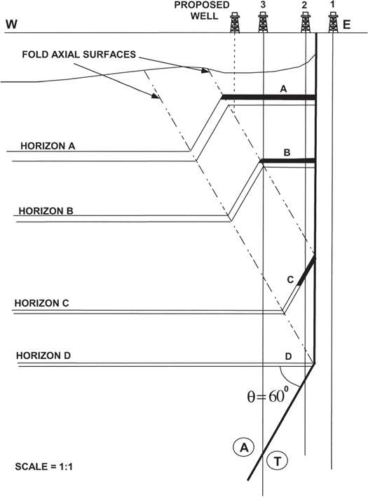
Figure 12-22 Company B geoscientists attempt to balance the structure and generate a strike-slip fault bend fold model that explains the anomalous bed dips and interval thickness changes at and below horizon C. In this model, the high bed dips occur at axial surfaces that define the flank of a monocline. Geoscientists propose a single shallow well at the A Sand to define the western limits of the field. This model shares properties with box and lift-off structures. (Published by permission of R. Bischke.)
The geoscientists can now complete the cross section shown in Figure 12-22, using the methods outlined in the previous section on compressional folding along strike-slip faults. Strata are deformed above the bend in the fault surface, so an axial surface emanates from this fault bend. They determine the dip of the axial surface by using the method described in the preceding section. Knowing that θ = 60 deg and ϕ = 30 deg, they use Figure 11-34 (right graph) to determine the axial surface angle γ to be 60 deg. As the regional dip is 0 deg, the actual dip of the axial surface is 60 deg. The axial surface projects upward at 60 deg from the bend in the fault (Fig. 12-22). The axial surface bisects the hinges of a fold, so by construction the A, B, and C Horizons dip at 60 deg through the no-seismic-data zone. The axial surface correlates to the western limit of the no-data zone on the seismic, and thus the no-data zone can result from changing bed dips and not from faulting, as assumed in the first interpretation.
Using similar reasoning with respect to Horizons A and B, the up-dip limit of the no-data zone can define a second axial surface. The axial surfaces are positioned as shown in Figure 12-22. As described earlier, seismic character correlation suggests the structural position of Horizons A and B are to the west (Fig. 12-20).
The Company B team assumes that the structure can be modeled using the Kink Method described in Chapter 10, and thus their cross section has more angular folds than the Company A cross section shown in Figure 12-21. Petroleum-scale structures, exhibiting a kink fold structural style, are common to the low temperature portions of fold and thrust belts (Suppe 1985; Boyer 1986). Furthermore, the Company B team are suspicious of the upturned beds imaged below the no-data seismic zone. The folding elevates high density and high velocity strata to a structural level that is higher than the equivalent beds located to the west of the no-seismic-data zone. Thus, the area below the region of high bed dips may be exhibiting velocity pull-up. In addition, as Company B concluded that the no-data zones result from folding and not faulting, there is no reason to postulate a fault-drag effect. They model the beds to the west of the no-data zone to be nearly flat surfaces.
The balanced interpretation presented by Company B also makes three assumptions. First, the no-data zone on the seismic data set results from high bed dips caused by folding. Second, folding causes changes in bed dips as well as in the different well log thicknesses. Third, folds in the low-temperature portions of mobile belts commonly exhibit kink geometry. The interpretation presented in Figure 12-22 has properties similar to lift-off or box folds (Chapter 10). The two interpretations contrast fundamentally. The interpretation presented by Company A emphasizes faulting, whereas the interpretation presented by Company B stresses folding.
The interpretation by Company B may not require any additional wells, depending on the areal extent of the reservoir and the drive mechanisms. However, to maximize development potential, one well is proposed to define the western limit of the accumulation in Horizon A. No wells are proposed to test the footwall plays in Horizons A and B (as presented by Company A), since the interpretation set has no closure in the footwall.
These two different interpretations will have a major impact on the exploration and development program. The interpretation shown in Figure 12-21 requires more wells and higher costs. It is based on negative evidence, limited structural knowledge, and a misunderstanding of the fold deformation in the footwall of the proposed secondary fault. Referring back to Chapter 1, we emphasize that a strong background in structural geology, not to be confused with an understanding of seismic interpretation, is a major component of a successful exploration or development program. This is particularly true in complex structural areas such as those discussed in this section.
The differences in the two interpretations result primarily from philosophical differences as to the approach used to resolve no-data zone problems and as to what represents real data. Rather than repeat many of the structural principles discussed in Tearpock et al. (1994) and this and other texts, we propose the following approach to evaluating conflicting or questionable structural interpretations. This approach is suggested by our experience in reviewing the results of many wells drilled in similar structural settings around the world.
Begin by examining interpretations to determine whether they honor all the data. Then look for obvious problems. Tearpock et al. (1994) present many quick-look techniques that aid in this analysis.
Certainly, geology can be complex, but where alternative solutions exist that honor all the data, the probable solution is commonly the less complex solution.
Valid interpretations of geological structures should be based on positive empirical evidence that confirms the presence of observed features. This requires an understanding of valid structural principles. The fault in Figure 12-21 may exist, but this interpretation is of high risk and is less likely. What constitutes negative evidence? A no-data zone on seismic, if used to support an argument, can qualify as an argument based on negative evidence. Thus, if faulting is proposed that is based on a no-data zone, then this argument is based on negative evidence. Again, this does not mean that the fault is not present; it means that this fault is a high-risk fault. Another way of approaching this problem is to consider what feature(s) on the data set will lower risk.
If an argument is based on negative evidence, ask yourself what positive evidence is required to support the argument. Throughout the world, most normal faults that dip at 70 deg image on seismic sections. Does a proposed fault in a no-data zone have a surface reflection or exhibit discontinuous reflections across the surface, and if not, why not? If the fault surface images, can a viable map of the fault surface be constructed that supports the faulting? Other observable features, such as large amounts of missing or repeated section in well log data, are direct evidence for faulting. These features lower fault risk. However, a change in dip on a dipmeter log can result from either faulting or the well crossing an axial surface.
Can another model better explain the observed features? This is where experience and training are important. Perhaps the no-data zone in our example results from high bed dips caused by folding and not by faulting. Geoscientists who work fold-thrust belts know that high bed dips are common to fold belts. Folding creates high bed dips that do not image on many seismic data sets. Furthermore, our experience shows that if faulting is present, then dip domain analysis (Chapter 10) typically locates direct evidence for the faulting in the form of bed dip discontinuities. If another explanation is as probable, or more probable, then caution is prudent. Risk the uncertainty accordingly. Good scientific work should yield better interpretations, resulting in more success at lower costs.
A structure similar to Figure 12-22 is shown in Figure 12-23 from Pecos Country, New Mexico, USA (Kelley 1971). The geological map of the region shows several long, arcuate northeast-southwest trending faults attributed to strike-slip displacements. This structure, called the Y-O Buckle, is bound by a near-vertical fault that contains a bend. A monoclinal fold forms above the bend in the fault, and below the bend the beds are not folded. The folded structures along these faults are subparallel to the surface trace of the faults, and they tend to exist at gentle bends in the faults. Thus, some of the folds appear to form at restraining bends. Field mapping demonstrates that the faults contain vertical separations that commonly change from normal to reverse separations along strike (Kelley 1971). The strata are deformed adjacent to the fault surfaces, often as disharmonic folds with near-vertical limbs (Figs. 12-22 and 12-23).
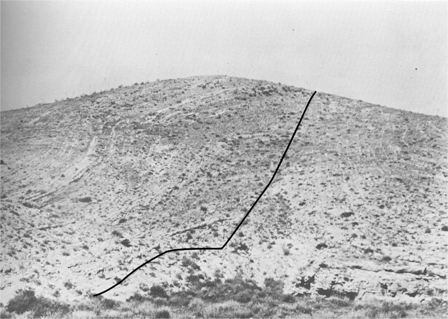
Figure 12-23 Box-like detachment fold in Pecos County, New Mexico, USA, along a long, arcuate fault system that appears to contain restraining and releasing bends. In the photograph, the strata are folded above the bend in the fault surface, similar to Figure 12-22. (From Kelly 1971. Published by permission of the New Mexico Bureau of Mines and Mineral Resources.)
Extensional Folding along Strike-Slip Faults
The balancing of releasing bends is similar to the balancing of restraining bends, except that the displacements are in the opposite direction. Rather than employing the techniques used in Chapter 10 on compressional structures, we use the techniques previously discussed for extensional structures (Chapter 11). We apply these ideas to a possible releasing bend in the classic Ridge Basin, southern California, that was carefully mapped by Crowell and his colleagues and students (Crowell 1950, 1982, 2003a, 2003b, 2003c). Crowell (2003c) and Link (2003) describe the detailed structure and stratigraphy of the basin along with the geological complications. In this section, we attempt to integrate surface dip data, seismic data, well log data, sedimentary data, and structural data into a model for Ridge Basin.
Ridge Basin Geology.
Ridge Basin formed along the northeastern boundary of the large right lateral San Gabriel strike-slip fault (Fig. 12-24), which was active during the late Miocene. The San Gabriel Fault is an inclined fault surface that strikes at about N40W and dips 50 deg to 70 deg to the northeast (Crowell 2003c). Piercing point evidence, consisting of offset belts of pre–Late Miocene rocks and structures, suggests that the San Gabriel Fault experienced about 60 to 80 km of strike-slip displacement (Crowell 1982, 2003c).

Figure 12-24 The compressional Transverse Range terminates at the right lateral San Gabriel Fault. (From Crowell 2003a. Published by permission of the Geological Society of America.)
Crowell (1974a, 1974b, 2003c) proposed that Ridge Basin formed as a result of a restraining bend located to the northwest of Ridge Basin and beneath the Frazier Mountain and Dry Creek Thrusts, that overthrust the northwestern part of Ridge Basin (Fig. 12-24). In his more recent model (Crowell 2003c) removed the extensional deformation from the basement that floors Ridge Basin and proposes squeezing and uplift at the stepover. As the evidence supports that 60 to 80 km of material moved through this restraining bend, a question arises as to why the active east-west-trending compressional Transverse Ranges terminate at the San Gabriel fault (Crowell 2003a) (Fig. 12-24); or why this east-west thrust faulting trend in the Transverse Ranges does not exist within domains 1 and 2 of Ridge Basin (Crowell, 1982, 2003c) (Fig 12-24; consult Restraining Bends section). An alternative interpretation of the regional data is that the right lateral San Gabriel Fault was originally part of the San Andreas Fault, and that modern strand of the San Andreas Fault has about 240 km of displacements (Ehlert 2003).
A seismic line presented by May et al. (1993) trends across the northwestern portions of Ridge Basin (Figs. 12-24 and 12-25). This line contains reflections that diverge toward an apparent listric normal fault that branches (splays) off the San Gabriel Fault. We call this proposed branch fault the Hungry Valley Fault. The deepest coherent reflections at about −10,000 feet on this depth-corrected seismic line dip at about 30 degrees, similar to the surface dips on the Geologic Map of Ridge Basin (Crowell 1982, 2003a, 2003b, 2003c). Most important, the line appears to image a rollover structure (May et al. 1993) (Fig. 12-26; also see Figs. 11-16 and 11-17). Typically, divergent dipping reflections dip toward listric normal faults and dip at about right angles to the normal fault. Therefore, the rolled-over reflections may dip toward a north-striking, branch normal fault that splays off the San Gabriel Fault (Link 2003).
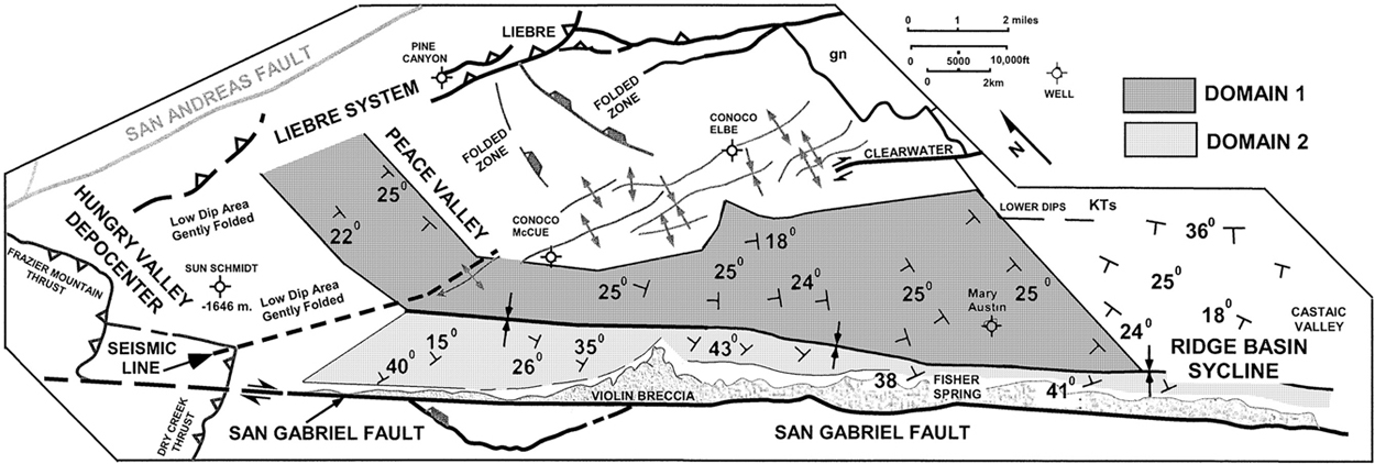
Figure 12-25 Generalized geologic map of Ridge Basin, California, modified after Crowell (1982, 2003a, Plate 1, a fold-out detailed map). Dip domain 1, located 1 to 3 km from the San Gabriel Fault, strikes north-south and dips to the west. Dip domain 2, adjacent to the San Gabriel Fault, dips to the north and is syncline-separated from dip domain 1. The two domains form the Ridge Basin syncline that subparallels the San Gabriel Fault. The gentle dips beneath Hungry Valley (in the west) are slightly folded by later compressional forces. Posted on the figure are the average values of the bed dips in the individual subdomains, along with the dip and strike directions. Average bed dips and strikes in domain 1 are 25W and N10E, and plunge of the synclinal axis is 24NW. Bed dips in domain 2 generally dip at high angles to the north, typically between the 25-deg to 45-deg range. (Published by permission of R. Bischke.)
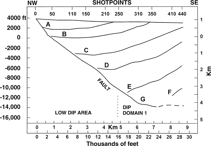
Figure 12-26 Tracing of depth-corrected seismic line across Ridge Basin that images an apparent half-graben rollover structure. The oblique seismic profile images reflections that contain apparent dips to the northwest. Where the profile crosses the low dip area of Hungry Valley, the hanging wall reflections directly above and adjacent to the fault surface exhibit low apparent dips. Seismic line crosses into domain 1 at about sp 250. See Figure 12-25 for the line location. Consult Link (2003) for a more detailed drawing of the seismic line. (After May et al. 1993. Published by permission of the Geological Society of America.)
This structural configuration favors an extensional releasing bend (Figs.12-9a and 12-11), subjecting Ridge Basin to a component of both dip-slip and strike-slip deformation. Furthermore, the Hungry Valley Fault, as shown in Figure 12-25, has normal separations that create accommodation space for the accumulation of the Ridge Basin sediments. This depocenter beneath Hungry Valley trends about north-south (Link 2003), so the Hungry Valley Fault also trends in a north-south direction (Link 2003). The Hungry Valley Fault was apparently responsible for the accumulation, rotation, and shingling of a section of Ridge Basin syntectonic sediments that are 14 km thick. The basin, however, was only about 5 km to 6 km deep (Crowell 2003c; Link 2003, 2003). Some deformational process was responsible for the rotation of these strata to dip at about 30 deg to the west (Crowell 2003a, 2003b, 2003c, Geologic Map of Ridge Basin and Geologic Cross-Section of Ridge Basin, profile A).
That this rotation is tectonic in nature is supported by the type of sedimentation in Ridge Basin, which involves the Peace Valley formation, and is about 9.0 km thick (Crowell, Geologic Cross-Section of Ridge Basin, profile A; Link 2003). Within the clastic units of the Peace Valley Formation the paleocurrent directions are to the southwest (Link 2003). According to Link et al. (1978) and Smyth (1982) the Peace Valley formation sediments are largely lacustrine, and 40% to 50% of the Violin Breccia consists of lacustrine fan deltas (Link 2003). These lacustrine deposits within the Peace Valley formations start with the shallow, freshwater Osito Canyon and Cereza Peak members and end with the Alamos Canyon and Posey Canyon members, which consist of brackish, deep-water lake sediments (Wood 1981; Link et al. 1978; Smith 1982). According to Smith (1982), the shallow fresh water deposits contain “wave-ripples, mudcrack casts, mammal tracks and arthropod burrows” and that these features are common. On Crowell’s Cross-Section A, these sediments extend for 15 km along the axis of the basin and downlap a thin veneer of Violin Breccia at high angles directly above horizontal basement. Thus, any model for Ridge Basin should account for these 30-deg dips through a 9.0-km thick lacustrine section.
A geological map of the basin published by Crowell (1982, 2003a, 2003b, 2003c) shows the following major features (Fig. 12-24). The geology adjacent to the San Gabriel Fault is dominated by the syntectonic Violin Breccia, deposited throughout the Late Miocene (Crowell 1982). Paralleling the breccia is the Ridge Basin syncline. The close association of the Violin Breccia with the Ridge Basin syncline suggests that the two features are related and that Ridge Basin syncline is a syntectonic feature. As Ridge Basin Group sediments onlap the flanks of the syncline, the stratigraphy supports the interpretation that the syncline is syntectonic (Link 2003). In the vicinity of Hungry Valley, the Pliocene sediments dip at gentle angles of 5 deg to 10 deg. These gently warped sediments were subject to late-stage Pliocene to Holocene folding that postdated the structure in areas north and northwest of dip domain 1 (May et al. 1993). Thus, the area surrounding Hungry Valley represents a gently dipping domain that was subsequently folded (Fig. 12-24).
Surface bed dips measured by Crowell define two large dip domains that dominate the structure to the southeast of Hungry Valley (dip domains 1 and 2 in Fig. 12-24). The Ridge Basin syncline partitions these domains. The largest of the domains (domain 1) dips to the west and lies about 1 to 3 km to the northeast of the San Gabriel Fault (Wood 1981; Crowell 1982, 2003c). The beds in domain 1 strike from 45 deg to 90 deg relative to the surface trace of the San Gabriel Fault (Fig, 12-24). We interpret this domain to dip toward the Hungry Valley Fault. The average bed dips, partitioned into smaller subdomains, are shown on Figure 12-24.
Dip domain 2 lies adjacent to the San Gabriel Fault and is syncline-separated from domain 1 (Fig. 12-25). In the northwest, this domain extends about 3 km to the northeast of the San Gabriel Fault, but to the southeast of Fisher Spring, the domain narrows to within 1 km of the fault zone. In domain 2 and in map view, the beds generally dip at high angles to the north and uniformly dip away from the San Gabriel Fault at oblique angles to the fault zone. Bed dips in this domain average 34 deg to the north. We emphasize, on typical rollover structures, from different areas of the world, beds dip toward normal faults at about right angles, not away from the fault surface at oblique angles. Thus, dip domains 1 and 2 form the Ridge Basin syncline. The oblique seismic line extends near the northwest portions of dip domain 2, located adjacent to the San Gabriel Fault, before entering dip domain 1, located about 4 km from the fault zone to the seismic line (Fig. 12-25).
Any model of the gross structural features in Ridge Basin should qualitatively and quantitatively explain the following structural features: (1) the approximate bed dips and the direction of the dips within the two domains; (2) the close association of the syntectonic Ridge Basin syncline with the syntectonic Violin Breccia and the San Gabriel Fault; (3) the processes that cause the strike of the beds to rotate up to 90 deg near the San Gabriel Fault zone, forming the Ridge Basin synclinal kink fold, and how these processes operate; and (4) how Ridge Basin was filled with at least 14 km of sediments, 7.5 km of which are lacustrine that presently dip at 30 deg to the west (the model also must be compatible with the stratigraphy of Ridge Basin [Link 2003] and with Goguel’s law of volume conservation [Chapter 10]); and (5) the interpretation should be restorable in that the cover should be restorable along with the basement (Chapter 10). Thus, one problem is how to restore the lacustrine sediments to the horizontal along with the basement without leaving a hole (see Crowell 2003a, Plate 1, Geologic Cross-Section of Ridge Basin, profile A). The dip domains and the syncline mapped by Crowell provide insight into the major tectonic processes associated with the San Gabriel Fault and the formation of Ridge Basin. As the subsurface geology is not well-constrained, we consider a solution to the Ridge Basin geology that assumes an extensional origin. This model will test the viability of an extensional origin for Ridge Basin based primarily on surface data. Other explanations may be possible, especially if more seismic data are acquired (consult Link 2003 for a review of the existing proposed models).
Geometry of Strike-Slip Extensional Folding.
The deformation of the hanging wall beds along a releasing bend differs from the deformation along a normal fault, as is seen in the perspective view diagram presented in Figure 12-27. An inclined strike-slip fault and a branch normal fault are shown. The dip of the branch normal fault surface decreases with depth. For purposes of convenience only, in Figure 12-27 we show this deep fault surface to be virtually horizontal. Displacement of the hanging wall block over the footwall causes the beds to be downthrown to the branch normal fault. These displacements also create accommodation space for growth sediments. According to the model, the beds adjacent to the strike-slip fault rotate downward at high and acute angles toward the branch fault. The beds forming to the right of the synclinal axis and located above the deep branch fault surface rotate toward the branch normal fault at right angles. The process generates a synclinally folded structure downthrown to the branch normal fault, with a synclinal axis that subparallels the strike of the strike-slip fault, mimicking the Ridge Basin geologic map (compare Fig. 12-27 to Crowell 2003a, Geologic Map of Ridge Basin, or Fig. 12-25).
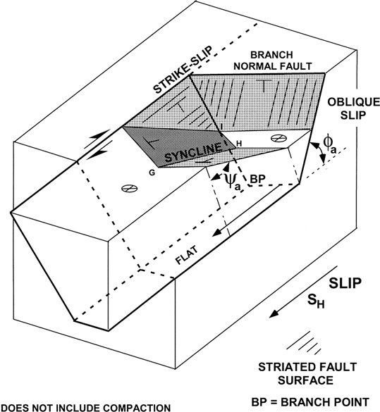
Figure 12-27 Perspective view of a synclinal, rollover structure forming along an inclined strike-slip fault. The strike-slip and branch normal faults form a releasing bend, and the strike-slip fault may be throughgoing. Slip vector is parallel to the strike direction of the strike-slip fault surface. The dip domain panel adjacent to the strike-slip fault dips away from the strike-slip fault, as the dip domain situated across the synclinal fold axis dips toward the branch fault surface. This fold style occurs along the San Gabriel Fault as the Ridge Basin syncline (Fig. 12-25 and Crowell 2003a, Plate 1, Geologic Map of Ridge Basin). Synclines may emanate from inclined releasing bends subject to large components of strike-slip motion. Figure is not drawn to scale. (Published by permission of R. Bischke.)
The detailed kinematics of the process are best shown in Figure 12-28, which is drawn such that the left-hand portion of the block is in the same vertical plane as the synclinal axis GH in Figure 12-27 (or plane GCDEH in Fig. 12-28b). In Figure 12-28a, slip on the strike-slip fault forms an inclined strike-slip fault surface, ABCD, and forms a nascent right-stepping releasing bend, fault surface ADF (Fig 12-28b) (also consult Figs. 11-2 and 12-30). The hanging wall in Figure 12-28 exhibits normal separations. In other words, the hanging wall block slips a small distance SH over the inclined strike-slip fault from point A to B, parallel to the strike of the strike-slip fault. This motion opens a small void beneath the hanging wall, a void which extends to the hidden, dashed line BC (Fig. 12-28a). The line BC was originally coincident with the line of bifurcation, AD, of the two fault surfaces (Fig. 12-28a). Thus, this small void exists above the surface ABCDF. As fault ADF is a normal fault subject to oblique-slip, this void is instantaneously filled by gravitational collapse (along Coulomb failure surface ψa in Figs. 12-28a and 12-30) of the hanging wall material onto the surface ABCDF (Fig. 11-2).

Figure 12-28 The kinematics of rollover folding above a releasing bend in a strike-slip fault. Slip component SH parallels the strike of the fault surface. (a) Slip from point A to point B causes the hanging wall cutoff BC to separate from footwall cutoff AD. The resultant motion opens a void beneath surface EBC, and the hanging wall will collapse by Coulomb shear onto the footwall. Point D' collapses onto point D along the apparent collapse angle ψa. (b) The resultant deformation causes the beds to dip away from the strike-slip fault surface in a direction perpendicular to the surface trace of the Coulomb collapse surface BG. Stereographic projection methods can determine the plunge of the line of bifurcation AD (branch normal fault in Fig. 12-29), based on knowledge of the strike and dip of the beds adjacent to the strike-slip fault and the apparent collapse angle ψa. Figure is not drawn to scale. (Published by permission of R. Bischke.)
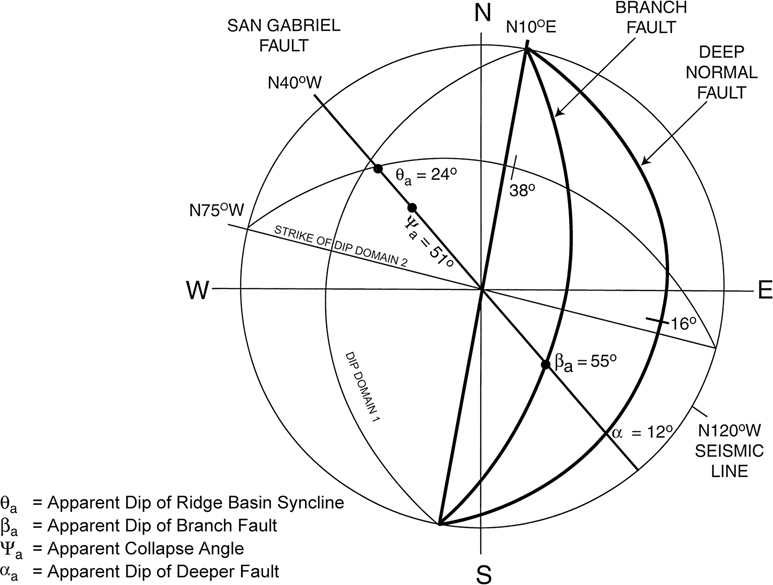
Figure 12-29 Stereoplot showing interpreted surface and subsurface structure at the Hungry Valley branch point (Fig. 12-32). Fault surfaces are bold lines and dip domains are thin lines on the projection. Constraints on the interpretation include the structural cross sections of Crowell (2003c), a seismic line, the surface trace of the San Gabriel Fault that trends at N40W, the measured average dip and strike of beds in dip domains adjacent to Hungry Valley, the N10W trend of the Hungry Valley depocenter (Link 2003), and the Sun Schmidt Well. The plunge of dip domain 2 and the Ridge Basin syncline (θa = 24 deg at N40W) help constrain the apparent dip (βa = 55 deg at N40W) of the Hungry Valley Fault that strikes at about N10E. The Hungry Valley Fault flattens at depth to form a listric fault surface. Measured dips in dip domain 1 (25W/N10E) and dip domain 2 (36NE/N75W) intersect to form the Ridge Basin syncline that trends subparallel to the San Gabriel Fault. Apparent bed dip of θa = 24NW constrains the bend in the normal fault surface, as does ϕa = 55 deg. (Published by permission of R. Bischke.)
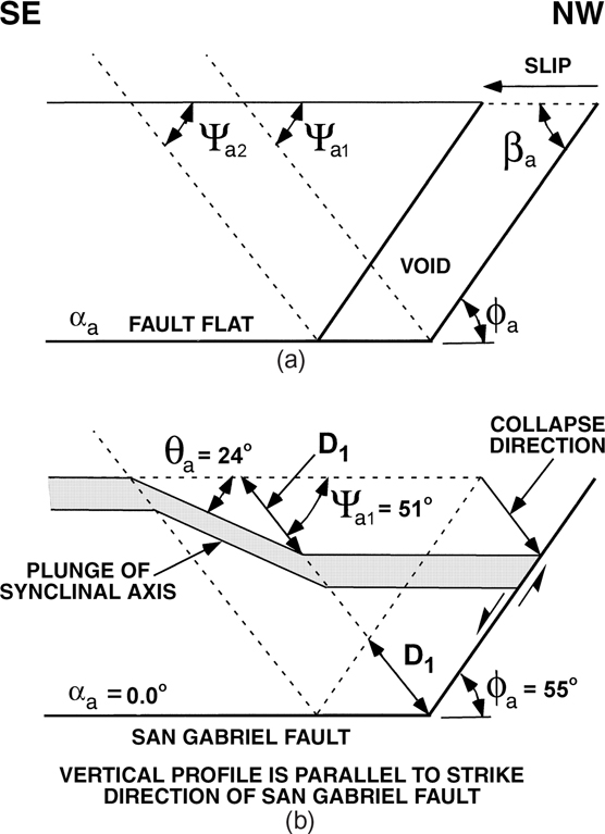
Figure 12-30 (a)–(b) Model for dip domain 2 adjacent and parallel to the San Gabriel Fault. (Published by permission of R. Bischke.)
In Figures 12-27 and 12-28b, line GH defines the plunge of the synclinal axial surface. Volume conservation therefore dictates that point D′ collapses onto the footwall in the plane containing line GH. As points D and D′ lie in the plane defined by the apparent Coulomb collapse angle ψa, point D′ collapses onto point D, forming a rollover. The collapse of the hanging wall onto the footwall causes the hanging wall beds to rotate and displace toward point E in Figure 12-28b, by bending along the active axial surface trace line BG. The active axial surface trace line BG is the surface expression of the inactive Coulomb collapse surface, BGC. The strike of the beds adjacent to the strike-slip fault define this deformation, which in the case of Ridge Basin is dip domain 2 in Figure 12-25. This deformation causes the beds to rotate away from the inclined strike-slip fault surface, forming one-half of a synclinal fold.
The remaining half of the synclinal fold is shown in Figure 12-27 as the surface above the fault flat that dips toward the branch normal fault. For clarity, that surface was not shown in Figure 12-28. Collapse along Coulomb shear surfaces causes the surface to the right of the synclinal axis to dip toward the branch fault. In the case of Ridge Basin, this surface is in dip domain 1 (Fig. 12-25).
If a dipping strike-slip fault and branch fault form a fault flat, as shown in Figure 12-27, then two dip domains form as the hanging wall block slides over the footwall. The beds adjacent to the strike-slip fault dip away from the strike-slip fault, and the beds above the fault flat dip toward the branch normal fault. This deformation results in a synclinal structure with an axial surface that trends subparallel to the surface trace of the strike-slip fault (Fig. 12-27). The Ridge Basin syncline exhibits this type of geometry (Fig. 12-25).
Geometry of the Hungry Valley Fault.
After determining the strike and dip of the proposed Hungry Valley Fault, which branches off the San Gabriel Fault, we model the dip of the deep normal fault beneath Ridge Basin. The modeling uses stereographic projection methods and extensional inverse balancing techniques, described in Chapter 11. As stated previously, near Hungry Valley, the San Gabriel Fault strikes at about N40W and dips to the northeast (Crowell 2003c) (Fig. 12-25). In addition, the trend of the Hungry Valley depocenter of about N10E (Link 2003), and the measured average N10E strike of the beds in domain 1, constrain the strike of the proposed Hungry Valley branch normal fault.
Notice on Figure 12-25 or on Crowell’s Geologic Map of Ridge Basin, that the synclinal axial surface near the seismic line subparallels the surface trace of the San Gabriel Fault. This allows the kinematics of strike-slip extensional folding to simply construct a balanced model for Ridge Basin (Fig.12-28b). Notice on Figure 12-28b that any vertical profile, oriented parallel to the surface trace of a dipping master strike-slip fault, contains a zero-deg (αa = 0.0) apparent dip for the deep fault surface (Fig. 12-30).
In other words, Figure 12-28b contains a vertical surface GCDEH that intersects the dipping master fault along dipping surface ABCD. The line of intersection between the two dipping surfaces GCDEH and ABCD, define the angle (αa). This apparent dip angle (α a) is independent of the dip on the dipping portion ABCD of the major strike-slip fault surface. This means that a general solution to the problem of strike-slip extensional folding is independent of the dip on the San Gabriel Fault surface. Also notice that from a comparison of Figure 12-28b to 12-30, the surface GHE (Fig 12-28b) allows a calculation of five apparent angles: (1) angle (αa), (2) angle (θa) = the apparent dip of the Ridge Basin syncline, (3) angle (ψa1) = the apparent dip of the Coulomb collapse angle, (4) angle (βa) = the apparent dip of the proposed Hungry Valley Fault, and angle, (5) (ϕa) = the apparent change in dip in the apparent fault surface. Also from Fig. 12-25, measurements exists for the calculation of (1) the strike of the San Gabriel Fault trending at N40W, (2) the strike of the branch fault from the averaged strikes of dip domain 1 located to the west of Peace Valley, and (3) the averaged dip and strike of domain 2 adjacent to the San Gabriel fault.
Lastly, the Coulomb collapse angle typically varies from 60 deg to 70 deg (Xiao and Suppe 1992; Bischke and Tearpock 1999). Here we assume a 65-deg Coulomb collapse angle. Next, we propose two balanced extensional folding models for Ridge Basin, one for dip domain 1, which traverses the deeper portions of the basin, and the second for dip domain 2, which parallels and cuts the San Gabriel Fault. Both domains are portrayed on a stereographic projection as thin lines (Fig. 12-29). We start with dip domain 2. These procedures may apply to other strike-slip faults (Fig. 12-33).
Model for Dip Domain 2.
We start with the best constrained data, the strike of the San Gabriel Fault and the Ridge Basin syncline, which is N40W on Figures 12-25 and 12-29. Next, the kinematics of pure strike-slip folding shown in Figures 12-27 and 12-28 permit a balanced and retrodeformable model of Ridge Basin along a vertical plane defined by line GCD (Fig. 12-28a). A profile in dip domain 2, constructed parallel to the surface trace of the San Gabriel Fault, can resolve the rollover structural geometry (Fig. 12-30). The problem is solvable if methods exist to measure (1) the apparent collapse angle ψa1 (Bischke and Tearpock 1999), (2) the apparent bed dip (θa), and (3) the apparent dip (αa), of the fault at depth. It then follows that the apparent fault bend (ϕa) in the fault surface is obtainable using either forward or inverse modeling techniques described in Chapter 11, in this case, the angles are measurable as ϕa = βa.
Notice in Figure 12-28b that line GHE lies in the plane that parallels the direction of fault slip and the Ridge Basin synclinal plunge GH (Fig. 12-27). Furthermore, material does not cross this plane. Also, notice that the active Coulomb collapse plane BGC intersects line GHE at an acute angle BG, located at the top of the hanging wall (Fig. 12-28a). This means that (1) not only will a balanced profile lie in the plane defined by the direction of fault slip, but (2) the Coulomb collapse angle (ψa), must be corrected for apparent dip (along with the other appropriate angles, such as apparent bed dip θa, βa, ψa1 (Fig. 12-30).
Assuming a Coulomb collapse angle of 65 deg, we first calculate the apparent collapse angle (ψa1), from the strike direction of the Coulomb collapse surface. We obtain this angle by measuring the strike direction of the beds in domain 2 adjacent to the San Gabriel Fault (Fig. 12-25). In the model in Figure 12-28, the calculated strike of the beds in domain 2 is parallel to the active axial surface trace line BG. The measured strike of the beds on dip domain 2 from Figure 12-25 averages N75W and is labeled on stereoplot in Figure 12-29. When θa is measured, then the bed dips in dip domain 1 and 2 can be predicted from the stereograph. Accordingly, and using stereographic projection methods, the true Coulomb collapse plane ψ dips at 65 deg and dips perpendicular to the active axial surface line BG, striking at N75W. However, on plane GCDEH (Fig. 12-28b), the apparent Coulomb collapse angle measurement is ψa1 = 51 deg and lies in a profile trending at N40W (Figs. 12-29 and 12-30). Next, using the same procedures to determine ψa1 (Fig. 12-30), we measure the apparent plunge angle θa of the Ridge Basin syncline, and the apparent dip of the branch fault, βa.
The plunge angle of the Ridge Basin syncline on plane GCDEH of Figure 12-28b is θa = 24 deg toward N40W (Fig. 12-30b). This value constrains the model as the great circles of dip domain 1, with dip domain 2, define the Ridge Basin syncline (Figs. 12-27 and 12-29). This 24-deg dip results in two conclusions. First, the great circle defining dip domain 2 determines the maximum dip for dip domain 2, which is about 38 deg to the north (Fig 12-29). Measured values from Figure 12-25 are 34N, striking at N85W, and thus calculated values from Figure 12-29 are close to measured values for dip domain 2. Second, in this solution, the branch fault dips at an apparent dip of 55 deg. SE (βa on Figs. 12-29 and 12-30).
In generating the model, we will later describe that the strike of the beds in dip domain 1 will be consistent with the strike of the Hungry Valley Branch Fault at about N10E. As stated in the previous paragraph, the apparent bed dip θa at the intersection of domains 1 and 2 defines the plunge angle of the Ridge Basin syncline (Figs. 12-29 and 12-30), which means that this 24-deg dip trending at N40W dip in domain 2 must be similar to the apparent dip in domain 1. This is required in order to maintain continuity at and across the synclinal axial surface. This apparent dip lies in the same vertical profile as the strike direction of the strike-slip fault and the Ridge Basin syncline, which in this case is the San Gabriel Fault treading at N40W (Figs. 12-25 and 12-29). If a profile lies in the strike direction of an inclined strike-slip fault, then the apparent fault dip αa = 0.0 deg (Fig 12-30a), and the apparent bend ϕa in the fault surface is equal to βa, the apparent dip of the Branch Fault (Fig. 12-30). Thus, the value for the apparent dip of the Hungry Valley Branch Fault can also be plotted on the stereographic projection with an apparent dip βa = 55 deg southeast (Fig. 12-29), and trending at S140E. We discuss in the next section that the trend of the branch fault is about N10E. Thus, the great circle through the apparent dip βa = 55 deg southeast defines the maximum dip of the branch fault at 59E/N10E (Fig. 12-29).
Inverse Modeling of Dip Domain 1 and the Branch Normal Fault.
Lastly, using the extension inverse theory (Chapter 11), and briefly described in this section, we first justify the shallow geometry of the Hungry Valley Fault from the geological data and then determine the dip of the deeper portion of the Hungry Valley Branch Fault, which forms the basal portions of Ridge Basin. We briefly describe the sedimentary evidence first.
According to the extensional model, the branch fault forms the western flank of the Hungry Valley depocenter. This assumption seems reasonable, as the stratigraphy of the basin (Link and Osborne 1982; Link 2003) predicts that a depocenter exists in the area of Hungry Valley (Figs. 12-25 and 12-26). A normal fault would form a depocenter. In addition, the direction of sedimentary transport into the Hungry Valley depocenter is from the north at about N10E (Link 2003). If we assume that the shallow portions of the proposed Hungry Valley Fault parallels the strike direction of dip domain 1, then the Hungry Valley Branch Fault may subparallel the present trend of the Hungry Valley basin. Using the observation that dipping beds, related to normal faulting, typically dipping at about a right angles to the strike of the normal fault (typical of rollover structures), measurements of strike of domain 1 (Fig. 12-25) predict a strike for the proposed Hungry Valley Fault is N10E, which is consistent with the sedimentary source direction (Link 2003).
Next, we estimate the strike of the branch fault using (1) the plunge angle of the Ridge Basin syncline of θa = deg toward the proposed Hungry Valley Fault, (2) the stereographic plot of the measured domain 1 bed dips, and (3) inverse modeling (Chapter 11). Inverse modeling, which is the reverse of forward modeling, employs surface bed dips or depth-corrected seismic data to predict deep subsurface fault geometry. The consequence of decoupling known surface data from the unknown deep fault geometry introduces uncertainty into the subsurface depth predictions. This uncertainty results primarily from measurement errors that are inherent in all inversion methods, including seismic and potential field methods. Although inversion methods contain error, they have the advantage of being able to make predictions.
The inversion of the surface dip data and the 55-deg southeast apparent dip on the Hungry Valley normal fault predicts the gross crustal structure beneath Ridge Basin. This exercise results in a generic and retrodeformable model of Ridge Basin (Chapter 11). Additional subsurface data, such as seismic profiles, are required to confirm these predictions.
Inverse theory requires a number of assumptions that include knowledge of the Coulomb collapse angle (typically between 60 deg and 70 deg), taken here to be 65 deg. This inversion uses a profile constructed parallel to the strike of the San Gabriel Fault using domain 1 dips in the direction of the San Gabriel Fault slip, which is N40W.
Retrodeformable Figure 12-31 represents any profile that trends in a direction of N40W across dip domain 1. This profile can trend adjacent to the Ridge Basin syncline or across Hungry and Peace Valleys in the northern portions of Ridge Basin (Fig. 12-25). As the profile parallels the slip direction of the San Gabriel Fault, the bed dip angle θa and deep normal fault dip angle αa are apparent dip angles. Domain 1 has an average bed dip θ of about 25 deg west, and it is separated from the gently dipping and folded Hungry Valley domain by an axial surface (Fig. 12-25). Correcting the bed dips in domain 1 to the profile direction of N40W results in an apparent dip θa =20 deg. This profile intersects the Hungry Valley Fault at an apparent dip of βa = 55 deg (Figs. 12-29 and 12-31).
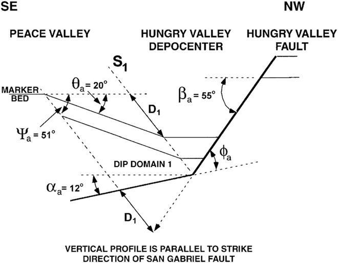
Figure 12-31 Inversion model for dip domain 1, used to calculate dip aa of the normal fault at depth. The listric normal fault causes the beds between Hungry and Peace Valleys to dip toward that fault, thus forming the Hungry Valley depocenter. The interpretation based on the surface dip data suggests that the 16-deg dipping normal fault may intersect the brittle-ductile transition beneath the volcanic Soledad Basin. (Published by permission of R. Bischke.)
To determine the apparent dip of the deeper part of the fault αa, use the methods described in the section Procedures for Projecting Large Normal Faults to Depth, in Chapter 11. As described in that section, simply project the distance D1 (Fig. 12-31) from the active to the inactive axial surface at the projection of the shallow fault surface. This procedure establishes the position and dip of the deeper part of the branch fault αa. In this case, the dip angle of the deep fault αa = 12 deg (Fig. 12-31). Using the stereonet (Fig. 12-29), this 12-deg apparent dip of the deeper fault, in a S140E direction, establishes the plane or great circle representing the deep normal fault. The true dip of the fault is 16 deg in a S100E direction (Fig. 12-29).
A normal fault dip of 16 deg projects to the east to intersect the brittle-ductile transition at a depth of about 20 km beneath the Soledad Basin that contains Tertiary volcanic rocks (Ehlert, 2003). This prior volcanic activity may have weakened the crust, facilitating the crustal extension. A generalized fault surface map for the Ridge Basin basement is shown in Figure 12-32. According to the model, hanging wall beds moving over the nonplanar fault surfaces deform at the bends in the fault surfaces. This motion replicates the main structural features and bed dips observed in Ridge Basin. Thus, the fault surface map represents a 3D fault surface model for the Ridge Basin structure (Fig. 12-25). The faults are tied to cross sections constructed by Crowell (2003c) and to the Sun Schmidt Well (Fig. 12-32). On Figure 12-32, all the fault surfaces are planar and the lines of fault intersection are determined with stereoplots. Where well control and seismic data are sparse, this procedure allows for the projection of fault surfaces over long distances and provides strong constraints on an interpretation surface dip data (Suppe 1983). Methods involving curved line projection techniques require dense data control and are not applicable to underconstrained data sets.
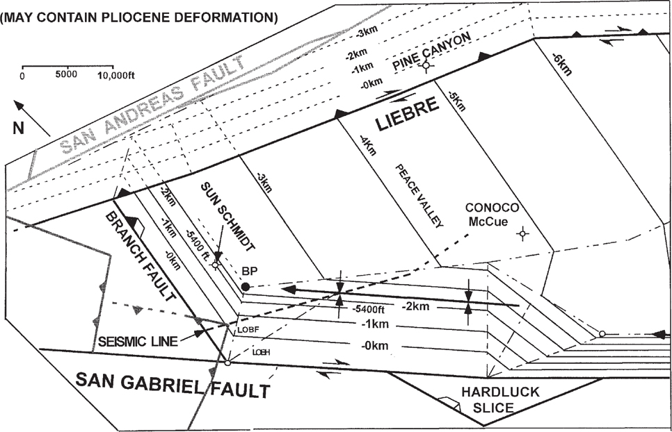
Figure 12-32 Generic fault surface map for the Ridge Basin basement, California. The interpretation of dip domain, seismic, and well data suggest that a branch fault forms a releasing bend in the area of Hungry Valley. This fault geometry, when combined with Coulomb collapse theory, models the general dip and strike pattern shown in Figure 12-25. The synclinal fold structure emanates from branch points (BP) located beneath Hungry Valley. Stereographic projection methods determine the fault plane intersections. (Published by permission of R. Bischke.)
The generalized fault surface map for the basement shown in Figure 12-32 is consistent with the major structural features and the bed dips observed in the Ridge Basin surface dips (Fig. 12-25). The generalized model shows that the Ridge Basin syncline emanates from the branch point (BP) of the San Gabriel Fault with the Hungry Valley Branch Fault. As the San Gabriel Fault dips at a higher angle in the southeast area of the map, the intersection of the deep normal fault with the San Gabriel Fault migrates to the south. This map may explain why domain 2 narrows to the southeast near Fisher Spring. The geometry of the San Gabriel Fault controls the position of the Ridge Basin syncline.
Tests of Model.
Measurements and stereographic projection can determine the true bed dip θ for dip domain 2, and measurements on profiles can determine apparent dip of the beds θa parallel to the San Gabriel Fault. This apparent dip angle θa lies in the same plane, defined by the great circle, as the true bed dip (Fig. 12-29). Near Hungry Valley, the strike of the beds in dip domain 2 is about N75W (Figs. 12-25 and 12-30). As the apparent dip of the beds (θa = 24 deg) lies in a profile that trends at N40W and in a plane that strikes at N75W, the maximum bed dip from the stereogram is determined to be 38 deg in a N15E strike direction (Fig. 12-29). This calculated value of 38N/N75W for the dip and strike of the beds in domain 2 is close to the observed average dips of 34N/N85W in dip domain 2 (Fig. 12-25).
Plotted on Figure 12-29 is dip domain 1, which dips and strikes at 25W/N10E. This plane intersects dip domain 2 to form the Ridge Basin syncline, which subparallels the surface trace of the San Gabriel Fault (compare Figs. 12-25 and 12-29). In Figure 12-29, the plane representing domain 1 (25W/N10E) intersects the plane representing dip domain 2 (36N/N75W) in a direction that is subparallel to the surface trace of the San Gabriel Fault and the Ridge Basin syncline at a direction of N43W. Thus, there is a good correspondence between the model and the observed surface bed dip data (Fig. 12-25 and Fig, 12-29).
Summary for Section
The balancing of strike-slip fault displacements is in its infancy and requires additional work involving restorable kinematic models that describe the structural styles observed along strike-slip fault zones. In Ridge Basin, the good correspondence between model-based predictions and observation is encouraging. However, these kinematic models should be subject to additional tests utilizing well-constrained data sets and viable fault surface maps. Nilsen and McLaughlin (1985) report that Ridge Basin contains some structures that are similar to Hornelen Basin in Norway and to portions of Little Sulphur Creek Basin in northern California (Fig. 12-33). Two of these basins contain a throughgoing strike-slip fault that bounds one flank of the basin, and talus and debris flow deposits exist adjacent to the strike-slip fault. These syntectonic breccias demonstrate growth through time. Paralleling the fault along the talus and debris flow deposits is a synclinal fold structure (Fig. 12-33). Nilsen and McLaughlin (1985) conclude that many of the world’s strike-slip extensional basins share similar tectonostratigraphic histories.
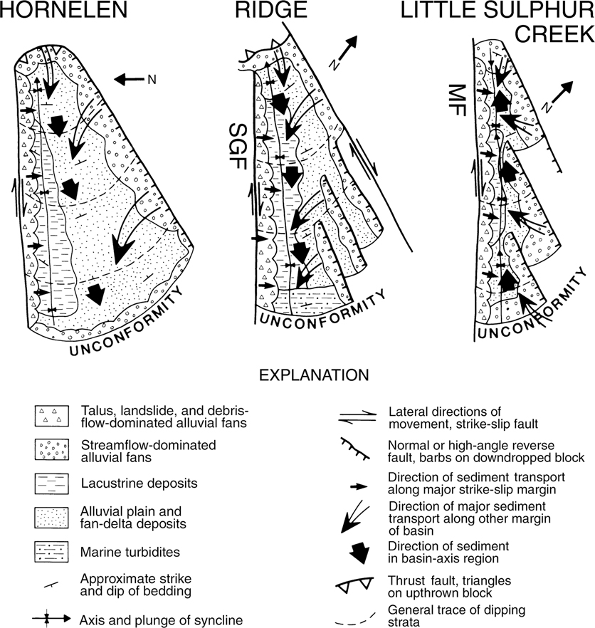
Figure 12-33 Hornelen Basin (Norway), Ridge Basin (southern California), and Little Sulphur Creek Basin (northern California), showing strike-slip fault and associated breccia and synclinal structure that parallel the strike-slip fault zone. (From Nilsen and McLaughlin 1985. Published by permission of the Society for Sedimentary Geology.)
When examining a strike-slip structure, we should ask ourselves how the structure and bed dips moved into their present positions. In this case, the question is, How did 25-to 30-deg lacustrine sediments downlap basement, along a N40W profile, across the deepest portions of the basin? A kinematic description of displacement of the structure is essential prior to embarking on the more theoretical analysis of how the structure reacted to stress and strain. The theory of elasticity is clear on this subject: kinematics is followed by dynamics (Obert and Duval 1967; Ramsay 1967). Clearly, scientists must develop the kinematic equations prior to formulating the tensor equations for stress and strain or differential equations. Structural studies that restrict the analysis to stress, while ignoring displacement analysis, seem questionable and unrealistic.
General Conclusions for Chapter 12
We are unaware of any method obtained from seismic or well log correlation data, or from models concerning stress theory (or the strain ellipsoid), that leads to resolving the state of stress on fault surfaces. Deductions concerning stress are not a viable exploration or prospect-generation tool. Stress is a mathematical concept, is invisible, and its direction cannot be deduced from neotectonic or older faulting data. Furthermore, clay analog models of strike-slip faulting contain a number of assumptions that affect the understanding of the structures and the styles of faulting that form along strike-slip faults. Clay models do not scale to the real earth (Hubbert 1937) and suffer from near-field boundary condition problems that impart contractional motions across a fault surface. The clay models do not correctly model the orientation or the regional distribution of real structures (Figs. 12-3, 12-4, and 12-5). Geoscientists are best served by applying correct interpretation procedures and mapping techniques to their data and prospects rather than relying on theoretical models involving stress or strain.
Early in an exploration project, geoscientists should concentrate their interpretation on observable and reliable data and should construct viable maps of recognizable fault surfaces. During the interpretation and construction of admissible fault surface maps, geoscientists will gain insight into the appropriate tectonic style affecting their area. When the mapped data lead geoscientists to a viable tectonic style, then geoscientists may employ a model to better understand and interpret the area. If interpreters approach a data set with preconceived ideas of the structure or bias toward a particular model, then the results of the exploration project are predictable—the interpretation and maps will conform to the preconceived ideas based on the model. A data-first, models-second approach is a more objective approach to any data set involving subsurface structure. Geoscientists then develop the appropriate model from the data rather than interpret the data using a convenient model. This approach is more likely to result in admissible interpretations and maps of the subsurface that are valid in 3D. This approach will minimize structural risks where exploration prospects exist.
Strike-slip fault interpretations should present direct evidence for horizontal displacements. As strike-slip faulting is a 3D problem, 2D seismic profiles can, at best, provide only suggestions of strike-slip faulting. However, the construction of viable maps of the faults is the first step in providing direct evidence for the horizontal displacements that are required for strike-slip interpretations. These viable maps of fault surfaces should show evidence of curved, or bent, fault surfaces. Strike-slip displacements at the bends will create restraining and releasing bends. Thus, restraining and releasing bends seem fundamental to the existence and understanding of strike-slip faults (Crowell 1974a, 1974b). Their ubiquitous presence along the major strike-slip fault zones presents direct evidence for strike-slip faulting. However, restraining and releasing bends may not record the total amount of strike-slip displacements. The bends may be obvious, such as the large bend along the Transverse Ranges of California (Fig. 12-10b). Alternatively, the bends may be subtle, like the bend at Loma Prieta along the San Andreas Fault (Fig. 12-18). Most important, these bends contain information that can confirm the presence of the horizontal displacements that accompany strike-slip faulting. If strike-slip faulting is present on a subsurface map, one only needs to look for the presence of restraining and releasing bends. Restraining bends should map as structural highs and releasing bends as structural lows. If evidence for restraining and releasing bends is not present on a regional scale subsurface map, then another interpretation may be warranted. If the strike-slip fault breaks the surface, then look for offset rock types on the surface geologic map (Crowell 1974a, 1974b).
We discussed several published techniques for recognizing strike-slip displacements. Three-dimensional regional and local restorations of strike-slip faulting may be supportive of horizontal displacements. Fault surface maps may show curved fault surfaces that form restraining and releasing bends. Folds form as the hanging wall beds move over curved fault surfaces (Bally et al. 1966; Rich 1934). Fault bend folding along strike-slip faults may prove useful in describing and analyzing structures in fault bends and along mapped fault surfaces. Balanced cross sections of restraining and releasing bends provide constraints on structural interpretation problems that lead to 3D structural validity and to admissible interpretations of subsurface data. Balanced cross sections of restraining and releasing bends should assist industry to generate high-quality prospects with reduced risk. In short, strike-slip fault interpretations should be subject to the same high-quality and rigorous interpretation techniques required of other styles of faulting.