

Post-deployment of DB2 with BLU Acceleration
In this chapter, we provide information about monitoring elements that you can observe from a DB2 with BLU Acceleration environment. We discuss how you can analyze and ensure that the environment is set up correctly for maximum performance. To demonstrate these concepts, we use the Cognos Sample Outdoors Warehouse example.
The following topics are covered:
6.1 Post-deployment of BLU Acceleration
With simplicity and ease of use being the main key objectives of the BLU Acceleration design, typical relational analytics database deployment tasks are greatly simplified. Database administrators no longer need to explicitly create user-defined indexes, or significantly tune databases to reach a state that is ready for production with excellent performance results.
With DB2 BLU Acceleration, analytic environments are automatically optimized with available hardware and are combined into a single registry variable, DB2_WORKLOAD=ANALYTICS. Basically create your column-organized tables, and then load and go. Chapter 5, “Performance test with a Cognos BI example” on page 169 showed decent performance results after data was loaded into column-organized tables, without any manual tuning effort.
The deployment of DB2 with BLU Acceleration is made easy through autonomics; the maintenance of BLU Acceleration is also straightforward. For DBAs, the DB2 process model is the same as you are used to. The same DB2 administration skills, APIs, backup and recovery protocols, and so on can all be kept as before. Also, you no longer must do many of the maintenance tasks because DB2 automatically does these for you.
Although DB2 with BLU Acceleration is easy to use with significantly less manual administration items, understanding how the database is configured and performing is useful. After a deployment, a DBA naturally wants to obtain the performance gain in the current workload with BLU Acceleration tables. DBAs can observe new monitoring elements to ensure that a deployed BLU Acceleration environment is working the way it should. This chapter focuses on these monitoring elements and some interesting BLU Acceleration administration tasks useful for DBAs.
6.2 Table organization catalog information
After deployment, the first item that you can check is the table organization of the converted tables listed in the catalog. DB2 10.5 adds a new column, TABLEORG, to the SYSCAT.TABLES catalog view. This single character value, displays the organization of each table: the letter “R” for row-organization or the letter “C” for column-organization.
Use the query in Example 6-1 on page 189 to see if your tables were created in BLU Accelerated columnar format.
Example 6-1 checking if table is in BLU Accelerated columnar format
SELECT
substr(tabschema, 1, 30) AS TABSCHEMA,
substr(tabname, 1, 30) AS TABNAME,
tableorg
FROM syscat.tables
WHERE tabschema ='<tabschema_name>';
Example 6-2 shows an excerpt of the output from the Cognos sample database after a BLU Acceleration deployment. The TABLEORG column shows “C” for all the column-organized tables in the GOSALESDW schema. The TABLEORG for those tables in the GOSALES schema are denoted as “R” to indicate traditional row-organized tables.
Example 6-2 Sample output of TABLEORG
TABSCHEMA TABNAME TABLEORG
-------------------- ------------------------------ --------
GOSALESDW SLS_RTL_DIM C
GOSALESDW SLS_SALES_FACT C
GOSALESDW SLS_SALES_ORDER_DIM C
GOSALESDW SLS_SALES_TARG_FACT C
GOSALES BRANCH R
GOSALES CONVERSION_RATE R
GOSALES COUNTRY R
GOSALES CURRENCY_LOOKUP R
6.3 BLU Acceleration metadata objects
To ensure optimal performance with BLU Acceleration, the DB2 engine creates and maintains metadata objects in the background. Although no DBA intervention is required for these metadata objects, it is beneficial to know about them.
6.3.1 Synopsis tables
One of the metadata object that gets created for BLU Acceleration is a data object called a synopsis table. It is created and populated automatically upon creation of a BLU Acceleration columnar table. This internal metadata table is maintained automatically during subsequent loads, imports, inserts, updates, and deletes of the column organized table for data-skipping purposes.
Before analyzing the structure of a synopsis table, first understand the synopsis table and how it is built. In DB2 10.5, when column-organized tables are created, a companion table (synopsis table) is also created by DB2, automatically. The synopsis table tracks the minimum and maximum column data values for each range of 1024 rows. The range of values that we store are specifically, from non-character columns and those character columns that are part of its primary or foreign key definitions. The size of the synopsis table is approximately 0.1% the size of the base table.
|
Note: Although not a requirement, loading pre-sorted data helps to cluster data and increase efficiency of synopsis tables.
|
Example 6-3 shows a synopsis table from a test environment. Note the structure of the table. Minimum and maximum values of non-character or key columns are stored, with the TSNMIN and TSNMAX values that indicate the row ranges (that is, tuple sequence numbers). In this example, when BLU Acceleration runs a query that looks for orders made in February 2014, it goes straight to the second two ranges of tuple sequence numbers (1024 - 3071) without having to scan through all the data.
Example 6-3 Sample excerpt of the output from a synopsis table
SHIP_DAY_KEYMIN SHIP_DAY_KEYMAX TSNMIN TSNMAX
--------------- --------------- ------------------- -------------------
20040113 20040115 0 1023
20040120 20040223 1024 2047
20040224 20040225 2048 3071
20040416 20040426 3072 4095
20040513 20061023 4096 5119
20061025 20061026 5120 6143
20061027 20061030 6144 7167
20061204 20061205 7168 8191
20061211 20061211 8192 9215
Synopsis tables are always created in the SYSIBM schema, with a naming convention like SYN%_<tablename>. To obtain a list of all synopsis tables that are created in the database, simply query a list of tables in the SYSIBM schema with its naming pattern, as shown in Example 6-4.
Example 6-4 Sample query to return a list of synopsis tables in database
select TABNAME, COLCOUNT
from SYSCAT.TABLES
where TABSCHEMA='SYSIBM' and TABNAME like 'SYN%';
Alternatively, to determine the name of the synopsis table that is created for a specific column-organized table, you can query the SYSCAT.TABLES catalog view by using the command shown in Example 6-5.
Example 6-5 Sample command and output to determine name of a synopsis table
select substr(TABSCHEMA,1,30) AS TABSCHEMA, substr(TABNAME,1,40) AS TABNAME
from SYSCAT.TABLES
where TABNAME like '%SLS_SALES_FACT';
TABSCHEMA TABNAME
------------------------------ ----------------------------------------
GOSALESDW SLS_SALES_FACT
SYSIBM SYN140325171836089285_SLS_SALES_FACT
2 record(s) selected.
Alternatively and to achieve similar results, you can query the SYSCAT.TABDEP catalog view as shown in Example 6-6. A new value to the dependent object metric is added to signify synopsis table objects (dtype='7').
Example 6-6 Synopsis Table Name Query
SELECT
bschema AS BLU_SCHEMA,
bname AS BLU_TABLENAME,
tabschema AS SYN_SCHEMA,
tabname AS SYN_TABLENAME
FROM syscat.tabdep
WHERE dtype = '7';
Example 6-7 shows an excerpt of the output of this query.
Example 6-7 Sample output of Synopsis tables from SYSCAT.TABDEP catalog view
BLU_SCHEMA BLU_TABLENAME SYN_SCHEMA SYN_TABLENAME
---------- -------------------- ---------- ------------------------------------
GOSALESDW SLS_RTL_DIM SYSIBM SYN140325171835493928_SLS_RTL_DIM
GOSALESDW SLS_SALES_FACT SYSIBM SYN140325171836089285_SLS_SALES_FACT
|
Tip: Synopsis tables only stores data value ranges for non-character columns or key columns. If a column with date values is a frequently queried column in a BLU Accelerated database, and it is currently defined as a character column, consider defining the column in the DATE data type instead. This ensures that the date column is included in the synopsis table and data-skipping is considered during a query process.
|
6.3.2 Pagemap indexes
DB2 with BLU Acceleration also automatically creates a data object called a pagemap index. It is also automatically maintained by the DB2 engine and is used by the engine to get the physical location of pages.
Example 6-8 shows a query that returns the associated pagemap index that is created for a particular BLU Acceleration table.
Example 6-8 Finding pagemap index query
SELECT
tabname,
indname,
indextype
FROM syscat.indexes
WHERE tabschema ='GOSALESDW'
ORDER BY tabname,indname;
Example 6-9 shows output. The CPMA index type represents column-organized page map (CPMA) index.
Example 6-9 Output of CPMA index types
TABNAME INDNAME INDEXTYPE
------------------------------ -------------------- ---------
SLS_RTL_DIM SQL14032517183566738 CPMA
SLS_SALES_FACT SQL14032517183626671 CPMA
SLS_SALES_ORDER_DIM SQL14032517183685697 CPMA
SLS_SALES_TARG_FACT SQL14032517183743802 CPMA
6.4 Storage savings
BLU Acceleration uses several compression algorithms to compress data, thus delivering significant storage savings. Besides saving storage, BLU Acceleration adaptive compression also helps improve query performance. The better your column-organized tables are compressed, the more data you can store in memory, thus reducing disk I/0 and improving query response time.
BLU Acceleration also has a unique vector-processing engine, which operates on compressed values rather than uncompressed values. This unique feature delivers much quicker query response times.
6.4.1 Table-level compression rates
Starting at a table level first, we examine the size and compression rates of BLU Acceleration tables. In particular, seeing the number of data pages that are saved through columnar compression is useful. DB2 10.5 creates the following monitor elements for columnar based data:
•COL_OBJECT_L_SIZE: Amount of disk space logically allocated for the column-organized data in the table, reported in kilobytes.
•COL_OBJECT_P_SIZE: Amount of disk space physically allocated for the column-organized data in the table, reported in kilobytes.
•COL_OBJECT_L_PAGES: Number of logical pages used on disk by column-organized data contained in this table.
These elements are reported by the ADMIN_GET_TAB_INFO table function, a standard administrative routine in DB2 10.5.
Also, an existing compression monitor element PCTPAGESSAVED is adapted for columnar tables. You can find the value of PCTPAGESSAVED for each BLU Acceleration table in the SYSCAT.TABLES catalog view. It provides an approximate percentage of pages saved in a table as a result of compression.
For row-based tables, NPAGES is normally used to determine the table size. However, for column-based BLU Acceleration tables, because NPAGES does not account for metadata or empty pages, it will underestimate the actual space usage, especially for small tables. You can obtain a more accurate value by adding the following key metric values from ADMIN_GET_TAB_INFO:
TOT_COL_STOR_SIZE = COL_OBJECT_P_SIZE + DATA_OBJECT_P_SIZE + INDEX_OBJECT_P_SIZE
This equation sums physical size of associated objects for a column-organized table:
•COL_OBJECT_P_SIZE is the physical size for column-organized data objects, including column-organized user data and empty pages.
•DATA_OBJECT_P_SIZE is the physical size for metadata objects including compression dictionaries created by DB2.
•INDEX_OBJECT_P_SIZE is the physical size for all index objects, including non-enforced keys and unique constraints if there is any, and pagemap indexes which is a metadata object that BLU uses to locate physical location of pages.
Example 6-10 is a query to retrieve the computed size (AS COLSIZE) of the column-organized tables along with the computed compression ratio (AS COMPRATIO).
Example 6-10 Table level compression analysis
SELECT
substr(a.tabschema,1,20) AS TABSCHEMA,
substr(a.tabname,1,20) AS TABNAME,
a.card,
b.data_object_p_size+ b.index_object_p_size+ b.col_object_p_size AS COLSIZE,
a.pctpagessaved,
DEC(1.0 / (1.0 - pctpagessaved/100.0),5,2) AS COMPRATIO
FROM
syscat.tables a,
sysibmadm.admintabinfo b
WHERE a.tabname = b.tabname
AND a.tabschema = b.tabschema
AND a.tabschema = 'GOSALESDW';
Example 6-11 shows an excerpt of the output.
Example 6-11 PCTPAGESSAVED and compression ratio sample output
TABSCHEMA TABNAME CARD COLSIZE PCTPAGESSAVED COMPRATIO
---------- -------------------- ---------- --------- ------------- ---------
GOSALESDW SLS_SALES_FACT 2999547946 158704640 83 5.88
GOSALESDW SLS_SALES_TARG_FACT 233625 9728 83 5.88
GOSALESDW DIST_PRODUCT_FORECAS 129096 4736 84 6.25
GOSALESDW MRK_PRODUCT_SURVEY_F 165074 5888 86 7.14
GOSALESDW SLS_PRODUCT_DIM 3000300 107520 86 7.14
In this example, we obtained a compression ratio (COMPRATIO) of approximately 5 - 7x, reducing storage and at the same time fitting more data into memory cache. If you find that PCTPAGESAVED has a value of -1, statistics might be outdated.
You can update the statistics by running the following DB2 command-line processor (CLP) command on the table in question:
db2 "RUNSTATS ON TABLE <BLU_TABLENAME> ON ALL COLUMNS WITH DISTRIBUTION ON ALL COLUMNS AND INDEXES ALL ALLOW WRITE ACCESS"
6.4.2 Column-level compression rates
Now that you have an idea of the column-organized tables storage footprint, and how effective the compression algorithms are, examining the tables further can help you understand how the data values are encoded at the column level. This section explores how to obtain the percentage of values that are encoded as a result of compression, for each column in our BLU Acceleration column-organized tables.
DB2 10.5 offers the PCTENCODED column in the SYSCAT.COLUMNS catalog view. It represents the percentage of values that are encoded as a result of compression for individual columns in a column-organized table. This information is collected and maintained as part of the automatic statistics gathering feature in BLU Acceleration.
By checking the value for each column in your columnar tables, you can measure and identify which columns have been optimally compressed. You can also determine if any column values were left uncompressed because of an insufficient utility heap during the data load. The SQL statement shown in Example 6-12 queries the column information and the percentage of values encoded in a Cognos sample GOSALESDW.SLS_SALES_FACT table.
Example 6-12 Column level compression analysis
SELECT
substr(tabname,1,20) AS TABNAME,
substr(colname,1,20) AS COLNAME,
substr(typename,1,10) AS TYPENAME,
length,
pctencoded
FROM
syscat.columns
WHERE tabschema ='GOSALESDW' and tabname='SLS_SALES_FACT'
ORDER BY 1,5 DESC;
Example 6-13 on page 196 shows output of the query. In this example, all columns in the GOSALESDW.SLS_SALES_FACT table are 100% encoded. This means, all column values are encoded by the compression dictionaries. This is the most ideal compression to achieve for best performance.
Example 6-13 Sample output of PCTENCODED
TABNAME COLNAME TYPENAME LENGTH PCTENCODED
-------------------- -------------------- ---------- ----------- ----------
SLS_SALES_FACT ORGANIZATION_KEY INTEGER 4 100
SLS_SALES_FACT CLOSE_DAY_KEY INTEGER 4 100
SLS_SALES_FACT ORDER_DAY_KEY INTEGER 4 100
SLS_SALES_FACT QUANTITY BIGINT 8 100
SLS_SALES_FACT PRODUCT_KEY INTEGER 4 100
SLS_SALES_FACT EMPLOYEE_KEY INTEGER 4 100
SLS_SALES_FACT GROSS_MARGIN DOUBLE 8 100
SLS_SALES_FACT RETAILER_KEY INTEGER 4 100
SLS_SALES_FACT PROMOTION_KEY INTEGER 4 100
SLS_SALES_FACT RETAILER_SITE_KEY INTEGER 4 100
SLS_SALES_FACT SALE_TOTAL DECIMAL 19 100
SLS_SALES_FACT SALES_ORDER_KEY INTEGER 4 100
SLS_SALES_FACT GROSS_PROFIT DECIMAL 19 100
SLS_SALES_FACT UNIT_COST DECIMAL 19 100
SLS_SALES_FACT ORDER_METHOD_KEY INTEGER 4 100
SLS_SALES_FACT UNIT_PRICE DECIMAL 19 100
SLS_SALES_FACT UNIT_SALE_PRICE DECIMAL 19 100
SLS_SALES_FACT SHIP_DAY_KEY INTEGER 4 100
18 record(s) selected.
If you see many columns, with a noticeable low value (or even 0) for PCTENCODED, the utility heap might have been too small when the column compression dictionaries were created.
If you see any columns or tables, where PCTENCODED has a value of -1, verify the following information:
•The table is organized by column.
•The statistics were collected and are up to date.
•The data was loaded into the table.
6.4.3 Automatic space reclamation
When data is deleted from a column-organized table, ideally, we want to return the pages, on which the deleted data resided, to table space storage, where they can later be reused by any table in the table space.
By setting the DB2_WORKLOAD registry variable to ANALYTICS, a default policy is applied, and the AUTO_REORG database configuration parameter is set so that automatic reclamation is active for all column-organized tables.
For environments where DB2_WORKLOAD registry variable is not set, you can set AUTO_REORG database configuration parameter to ON to enable automatic column-organized tables space reclamation. If for any reason you prefer to keep the AUTO_REORG configuration parameter disabled, you can manually reclaim space by using the REORG TABLE command and specifying the RECLAIM EXTENTS option for that command. As with most background processes, BLU Acceleration uses an automated approach.
If required, you can monitor the progress of a table reorganization operation with the reorganization monitoring infrastructure. The ADMIN_GET_TAB_INFO table function returns an estimate of the amount of reclaimable space on the table, which you can use to determine when a table reorganization operation is necessary.
To determine whether any space can be reclaimed, you might use the query shown in Example 6-14, which returns the amount of reclaimable space for a BLU Acceleration column-organized table.
Example 6-14 Estimate reclaimable space
SELECT
tabname,
reclaimable_space
FROM table(sysproc.admin_get_tab_info('GOSALESDW','SLS_SALES_FACT'));
Example 6-15 shows output where no space needs to be reclaimed. This is as expected in an environment where AUTO_REORG is enabled. A DB2 daemon runs in the background and frequently checks and reclaims any empty extents that can be reclaimed automatically.
Example 6-15 Reclaimable space for a table
TABNAME RECLAIMABLE_SPACE
------------------------------ --------------------
SLS_SALES_FACT 0
1 record(s) selected.
6.5 Memory utilization for column data processing
Another key feature of DB2 with BLU Acceleration is scan-friendly memory caching. Most database systems have memory caching, but they tend to be configured for transaction processing rather than analytical. Transaction processing systems tend to use paging algorithms, such as least recently used (LRU) and most recently used (MRU). This usually results in keeping the data most recently referenced, in memory and getting rid of older, less frequently accessed data from memory to disk.
DB2 with BLU Acceleration introduces a new scan-friendly, analytics-optimized, page-replacement algorithm. It detects data access patterns, keeps hot data in buffer pools as long as possible, and minimizes I/O. It also works well with traditional row-based algorithms in mixed workload environments. As with most admin tasks with BLU Acceleration, the DBA does not have to do any tasks here, BLU Acceleration automatically adapts the way it caches data based on the organization of the table being accessed. No optimization hints, no configuration parameters to set, it all happens automatically.
6.5.1 Column-organized hit ratio in buffer pools
Although BLU Acceleration delivers accelerated performance using unique analytics-optimized algorithms and buffer pool caching, a prudent task is to always monitor the memory aspects of your database. Understand how well your workloads use buffer pool reads versus physical reads.
Table A-1 on page 409 indicates new monitor elements that are added to DB2 10.5 and that you can use to monitor buffer pool and prefetch usage by column-organized tables. Rather than individually querying each of these metric values, DB2 10.5 automatically creates administrative views that provide a condensed representation of the monitor elements, displaying the highlights, and providing several standard calculations that are of most interest, such as buffer pool hit ratio. These views are similar to table functions because they return data in table format. However, unlike table functions, they do not require any input parameters.
The MON_BP_UTILIZATION administrative view returns the following columnar buffer pool information:
•COL_PHYSICAL_READS
This is the number of column-organized table data pages read from the physical table space containers.
•COL_HIT_RATIO_PERCENT
This is the column-organized table data hit ratio (percentage of time that the database manager does not have to load a page from disk for the request).
You can use the SQL query in Example 6-16 on page 199 to observe how the buffer pool is performing.
Example 6-16 SQL query for observing the buffer pool performance
SELECT
varchar(bp_name,20) AS BUFFER_POOL,
col_physical_reads,
col_hit_ratio_percent
FROM
sysibmadm.mon_bp_utilization;
Example 6-17 shows output from a Cognos Sample Outdoors sample database. In this example, the GOSALES_BP where the column-organized GOSALESDW schema resides has 96.9% COL_HIT_RATIO_PERCENT. This means for approximately 96.9% of the time, the workload was able to process the column-organized data from the buffer pools without reading the physical disk. Ideally, we want the COL_PHYISICAL_READS to be as low as possible, and the COL_HIT_RATIO_PERCENT to be as close to 100% as possible.
Example 6-17 Bufferpool columnar performance metrics
BUFFER_POOL COL_PHYSICAL_READS COL_HIT_RATIO_PERCENT
-------------------- -------------------- ---------------------
IBMDEFAULTBP 0 -
GOSALES_BP 9413531 96.90
IBMSYSTEMBP4K 0 -
IBMSYSTEMBP8K 0 -
IBMSYSTEMBP16K 0 -
IBMSYSTEMBP32K 0 -
6 record(s) selected.
6.5.2 Prefetcher performance
The prefetch logic for queries that access column-organized tables is used to asynchronously fetch only those pages that each thread reads for each column that is accessed during query execution. If the pages for a particular column are consistently available in the buffer pool, prefetching for that column is disabled until the pages are being read synchronously, at which time prefetching for that column is enabled again.
Prefetch monitor elements (listed in Table A-1 on page 409) can help you track the volume of requests for data in column-organized tables that are submitted to prefetchers, and the number of pages that prefetchers skipped reading because the pages were in memory. Efficient prefetching of data in column-organized tables is important for mitigating the I/O costs of data scans.
You can use the SQL query in Example 6-18 to observe how the prefetchers are performing. A reference to what each column represents is in Table A-1 on page 409. Typically, we are looking for small values to be returned for prefetch waits and prefetch wait times, which indicates minimal I/O as pages already in the buffer pool.
Example 6-18 SQL query for observing prefetch performance
SELECT
bp_name,
pool_queued_async_col_reqs AS COL_REQS,
pool_queued_async_col_pages AS COL_PAGES,
pool_failed_async_col_reqs AS FAILED_COL_REQS,
skipped_prefetch_col_p_reads AS SKIPPED_P_READS,
prefetch_wait_time,
prefetch_waits
FROM table(sysproc.mon_get_bufferpool('',-1));
Example 6-19 shows output of the query. In this example, we focus on the GOSALES_BP buffer pool that handles the sample Cognos analytic workloads for the test. From this output, we observe a total of 13,594,221 (pool_queued_async_col_reqs AS COL_REQS) column-organized pages that are requested from the workload.
Of the total of pages requested, approximately 5,368,715 pages (skipped_prefetch_col_p_reads AS SKIPPED_P_READS) are skipped from physical reads because those pages are already in the buffer pool. This means that approximately 40% of data was already found in the buffer pool as the Cognos workload was run.
We examine the pool_queued_async_col_reqs element (AS COL_REQS in output). There are total of 3,146,216 column-organized requests from the workload. Of all the requests, only 280657 (prefetch_waits) requests need to wait for the prefetcher to load data to buffer pool. This means, approximately 9% of the total requests require a wait from the prefetcher. This can be a result of the DB2 prefetcher being able to detect and determine the correct type of prefetch to use.
If we take the prefetch_wait_time divided by the prefetch_waits, we get the average time spent for prefetcher to load data onto the buffer pool. From our example, only about 35 milliseconds are spent for each prefetch. Ideally, you want as short a prefetch wait time as possible in an optimal environment.
Example 6-19 Prefetcher performance sample output
BP_NAME COL_REQS COL_PAGES FAILED_COL_REQS SKIPPED_P_READS PREFETCH_WAIT_TIME PREFETCH_WAITS
-------------- -------- --------- --------------- --------------- ------------------ --------------
IBMDEFAULTBP 0 0 0 0 179 25
GOSALES_BP 3146216 13594221 0 5368715 9845548 280657
IBMSYSTEMBP4K 0 0 0 0 0 0
IBMSYSTEMBP8K 0 0 0 0 0 0
IBMSYSTEMBP16K 0 0 0 0 0 0
IBMSYSTEMBP32K 0 0 0 0 0 0
6 record(s) selected.
6.5.3 Monitoring sort memory usage
Monitoring sort memory usage is important to ensure that BLU Acceleration is performing optimally against your analytical queries. In earlier chapters, we learned that BLU Acceleration uses a set of innovative algorithms to join and group column-organized data in an exceptionally fast manner, resulting in the dramatic performance improvements in analytic workloads. These algorithms utilize hashing techniques, which in turn, require sort memory to process. Therefore, BLU Acceleration does typically require more sort memory than traditional row-organized databases. The primary sort memory consumers are JOINs and GROUP BY operations.
In an environment with BLU Acceleration, there are a few factors that affect performance of sort memory consumers:
•SORTHEAP database configuration parameter
SORTEHAP is generally set to a higher number with self-tuning disabled when BLU Acceleration is enabled on a database. This parameter limits the maximum number of memory pages that sort heap memory can use.
•SHEAPTHRES_SHR database configuration parameter
SHEAPTHRES_SHR is also set to a higher number with self-tuning disabled when BLU Acceleration is enabled on a database. Together with the SHEAPTHRES database manager parameter set to 0, this parameter specifies the total amount of database shared memory that is available for sort memory consumers at any given time. It controls the shared sort memory consumption at the database level. When overall sort memory usage approaches the SHEAPTHRES_SHR limit, memory throttles and sort memory requests might get less memory than required. This can lead to data spilling into temporary tables and performance degrade. When overall memory usage exceeds the SHEAPTHRES_SHR limit, queries can fail.
•The number of sort memory consumers running concurrently.
To monitor and ensure that sort memory usage is optimal in your BLU Acceleration environment, you can monitor behaviors of various sort memory consumers and the concurrency.
Monitoring sort usage
The following monitoring elements return the overall sort memory usage for a database:
•SORT_SHRHEAP_ALLOCATED
Total amount of shared sort memory currently allocated in the database. When no active sort is running at a given time, SORT_SHRHEAP_ALLOCATED reports a value of 0.
•SORT_SHRHEAP_TOP
The high watermark for database-wide shared sort memory.
Example 6-20 shows a SQL query that reports the currently allocated shared sort heap at a given time and the high watermark shared sort heap usage. The high watermark value gives a baseline on the maximum sort memory that the system requires for the workload.
Example 6-20 Currently allocated and maximum shared sort heap usage
SELECT SORT_SHRHEAP_ALLOCATED, SORT_SHRHEAP_TOP
FROM TABLE(MON_GET_DATABASE(-1));
SORT_SHRHEAP_ALLOCATED SORT_SHRHEAP_TOP
---------------------- --------------------
51690 71009
1 record(s) selected.
Monitoring active sort operations
The following monitoring elements report the currently active sort operations being executed on the database:
•ACTIVE_SORTS
Number of sorts in the database that are currently running and consuming sort heap memory.
•ACTIVE_HASH_JOINS
Total number of hash joins that are currently running and consuming sort heap memory.
•ACTIVE_OLAP_FUNCS
Total number of OLAP functions that are currently running and consuming sort heap memory.
•ACTIVE_HASH_GRPBYS
Total number of GROUP BY operations that use hashing as their grouping method that are currently running and consuming sort heap memory.
Example 6-21 shows a SQL query that reports the total number of active sort operations currently running and consuming sort memory:
Example 6-21 Total number of active sort operations currently running and consuming sort memory
SELECT
(ACTIVE_SORTS + ACTIVE_HASH_JOINS + ACTIVE_OLAP_FUNCS + ACTIVE_HASH_GRPBYS) AS TOTAL_ACTIVE_SORTS
FROM TABLE(MON_GET_DATABASE(-1));
TOTAL_ACTIVE_SORTS
--------------------
6
1 record(s) selected.
Using these monitoring elements, you can determine the maximum number of concurrent sort memory operations. If concurrency is high, consider a lower ratio of SORTHEAP and SHEAPTHRES_SHR database configuration parameters. For example:
•Set SORTHEAP to a value of (SHEAPTHRES_SHR/5) for low concurrency
•Set SORTHEAP to a value of (SHEAPTHRES_SHR/20) for higher concurrency
Monitoring total sort memory and overflows
The following monitoring elements report the total number sort memory consumers executed on the database:
•TOTAL_SORTS
Total number of sorts that have been executed.
•TOTAL_HASH_JOINS
Total number of hash joins executed.
•TOTAL_OLAP_FUNCS
Total number of OLAP functions executed.
•TOTAL_HASH_GRPBYS
Total number of hashed GROUP BY operations.
The following monitoring elements report the total number of sort overflows on the database. When there are sort overflows, results are spilled to the system temporary table which causes undesirable disk access. This degrades performance and should be avoided.
•SORT_OVERFLOWS
The total number of sorts that ran out of sort heap and may have required disk space for temporary storage.
•HASH_JOIN_OVERFLOWS
The number of times that hash join data exceeded the available sort heap space.
•OLAP_FUNC_OVERFLOWS
The number of times that OLAP function data exceeded the available sort heap space.
•HASH_GRPBY_OVERFLOWS
The number of times that GROUP BY operations use hashing as their grouping method and exceeded the available sort heap memory.
Example 6-22 shows an SQL query that reports the total sort usage and the number of sort operations overflowed.
Example 6-22 Total sort consumers and number of sort operations overflowed
SELECT
(TOTAL_SORTS + TOTAL_HASH_JOINS + TOTAL_OLAP_FUNCS + TOTAL_HASH_GRPBYS) AS TOTAL_SORT_CONSUMERS,
(SORT_OVERFLOWS + HASH_JOIN_OVERFLOWS + OLAP_FUNC_OVERFLOWS + HASH_GRPBY_OVERFLOWS) AS TOTAL_SORT_CONSUMER_OVERFLOWS
FROM TABLE (MON_GET_DATABASE(-1));
TOTAL_SORT_CONSUMERS TOTAL_SORT_CONSUMER_OVERFLOWS
-------------------- -----------------------------
178 0
1 record(s) selected.
Optionally, you can use the two values to compute the percentage of sort memory operations that spilled to disk. To do so, divide the total sort memory consumers overflowed by the total number of sorts used. If the sort overflow percentage is high, there is a large percentage of sort operations throttled and spilled to disk.
In this case, consider the following possibilities:
•Increase the SHEAPTHRES_SHR database configuration parameter so that more memory is available for concurrent sort operations.
•Adjust the Workload Management concurrency limits for the workload to reduce the number of concurrently executing sort operations.
For more details of monitoring sort consumer overflows, see this web page:
6.6 Workload management
From DB2 9.5, a set of features was introduced into the DB2 engine, in the form of DB2 Workload Manager (WLM). With DB2 WLM, you can treat separate workloads (applications, users, and so on) differently, and provide them with different execution environments to run in. It improves the workload management process by ensuring priority workloads get the most resources allocated to them.
6.6.1 Automatic workload management
DB2 10.5 with BLU Acceleration builds on DB2 Workload Manager (WLM) and includes automated query resource consumption controls to deliver even higher performance to your analytic database environments. With BLU Acceleration, there is a threshold limit on the number of “heavyweight” queries that can run against a database at any one time. This ensures that heavier workloads that use column-organized data will not overload the system and affect the lighter weight queries.
Several default workload management objects are created for new or converted BLU Acceleration databases. Particularly, a new service subclass called SYSDEFAULTMANAGEDSUBCLASS is enabled for analytics workload. It is specifically for handling heavy, long running queries and is bounded by the SYSDEFAULTCONCURRENT threshold. Table 6-1 summarizes the WLM components for this service subclass.
Table 6-1 WLM components for the SYSDEFAULTMANAGEDSUBCLASS
|
WLM component
|
Name
|
Description
|
|
service subclass
|
SYSDEFAULTMANAGEDSUBCLASS
|
Controls and manages heavyweight queries.
|
|
threshold
|
SYSDEFAULTCONCURRENT
|
Controls the number of concurrently running queries that are running in the SYSDEFAULTMANAGEDSUBCLASS.
|
|
work class
|
SYSMANAGEDQUERIES
|
Identifies the class of heavyweight queries to control. This includes queries that are classified as READ DML (a work type for work classes) and that exceed a timeron threshold that reflects heavier queries.
|
|
work class set
|
SYSDEFAULTUSERWCS
|
Identifies the class of heavyweight queries to control.
|
These workload management objects help control the processing of light and heavyweight queries. Figure 6-1 illustrates how the automatic WLM process works for analytic workloads.
Figure 6-1 Automatic WLM process for BLU Acceleration
Any read-only queries submitted to the system are categorized based on the query cost estimate generated by DB2 cost-based optimizer into a managed and unmanaged query classes. Lightweight queries that are below a defined cost (and non-read-only activities) are categorized as unmanaged and are allowed to enter the system with no admission control. This avoids a common problem with queuing approaches in which the response time of small tasks that require modest resources can suffer disproportionately when queued behind larger, more expensive tasks.
For heavyweight queries above the timeron cost, DB2 categorizes these as managed, and applies an admission control algorithm that operates based on the processor parallelism of the underlying hardware. When a certain number of managed queries are running on the server, further submitted queries are queued if the current number of long-running queries is at the upper limit to optimize the current hardware. This is done transparently to the user, who sees only the resulting performance benefit from a reduction in spilling and resource contention among queries.
Automatic SYSDEFAULTCONCURRENT threshold for heavy queries
The threshold limit, SYSDEFAULTCONCURRENT, is automatically enabled on new databases if you set the value of the DB2_WORKLOAD registry variable to ANALYTICS. Its value is calculated during database creation or when database is autoconfigured, based on system hardware attributes such as the number of CPU sockets, CPU cores, and threads per core.
This limit is captured in the SYSCAT.THRESHOLDS catalog view. To retrieve this limit, you can use the query shown in Example 6-23.
Example 6-23 WLM threshold
SELECT
substr(thresholdname,1,25) AS THRESHOLDNAME,
SMALLINT(maxvalue) AS MAXVALUE,
decode(enforcement,'W','WORKLOAD','D','DATABASE','P','PARTITION',
'OTHER') AS ENFORCEMENT
FROM syscat.thresholds
WHERE thresholdname='SYSDEFAULTCONCURRENT';
Example 6-24 shows output of the query. In this example, the maximum number of heavy queries that can run at the same time is 14, enforced on database level.
Example 6-24 System WLM concurrent limit
THRESHOLDNAME MAXVALUE ENFORCEMENT
------------------------- -------- -----------
SYSDEFAULTCONCURRENT 14 DATABASE
1 record(s) selected.
Changing threshold when hardware specs has changed
If your hardware specification has changed since SYSDEFAULTCONCURRENT threshold was last auto-configured, you can use the configuration advisor to generate a new threshold suitable for your new hardware. Example 6-25 shows an AUTOCONFIGURE APPLY NONE command to review the recommended changes:
Example 6-25 Review autoconfigure recommended values
db2 AUTOCONFIGURE APPLY NONE
Current and Recommended Values for System WLM Objects
Description Current Value Recommended Value
-----------------------------------------------------------------------------
Work Action SYSMAPMANAGEDQUERIES Enabled = Y Y
Work Action Set SYSDEFAULTUSERWAS Enabled = Y Y
Work Class SYSMANAGEDQUERIES Timeroncost = 1.50000E+05 1.50000E+05
Threshold SYSDEFAULTCONCURRENT Enabled = Y Y
Threshold SYSDEFAULTCONCURRENT Maxvalue = 14 16
If the recommended value has changed, you can use the command in Example 6-26 to change the current SYSDEFAULTCONCURRENT threshold to a recommended value. This example demonstrates changing the threshold to a recommended value of 18 as an example.
Example 6-26 Changing SYSDEFAULTCONCURRENT threshold
db2 ALTER THRESHOLD SYSDEFAULTCONCURRENT
WHEN CONCURRENTDBCOORDACTIVITIES > 16 STOP EXECUTION
Display total CPU and queue time for each service subclass
If you want to drill-down further to observe how each workload management service class is performing, specifically, the wait time that is spent in the SYSDEFAULTMANAGEDSUBCLASS where heavy queries are run, use the command shown in Example 6-27.
Example 6-27 SQL statement to determine CPU costs and total queue time in each service subclass
SELECT
service_superclass_name,
service_subclass_name,
sum(total_cpu_time) as TOTAL_CPU,
sum(wlm_queue_time_total) as TOTAL_QUEUE_TIME
FROM TABLE(MON_GET_SERVICE_SUBCLASS('','',-2)) AS t
GROUP BY service_superclass_name, service_subclass_name
ORDER BY total_cpu desc;
This command returns the total CPU time, and the total queue time for every WLM service class, ordered by CPU time.
Example 6-28 shows output. The WLM_QUEUE_TIME_TOTAL metric indicates the accumulated time that queries wait on concurrency threshold. Ideally, WLM_QUEUE_TIME_TOTAL should be as low as possible.
Example 6-28 Service subclasses and their total CPU costs and queue time
SERVICE_SUPERCLASS_NAME SERVICE_SUBCLASS_NAME TOTAL_CPU TOTAL_QUEUE_TIME
---------------------------- ---------------------------- ------------ ------------------
SYSDEFAULTMAINTENANCECLASS SYSDEFAULTSUBCLASS 65179497 0
SYSDEFAULTUSERCLASS SYSDEFAULTMANAGEDSUBCLASS 35227720522 0
SYSDEFAULTUSERCLASS SYSDEFAULTSUBCLASS 198413509 0
SYSDEFAULTSYSTEMCLASS SYSDEFAULTSUBCLASS 0 0
4 record(s) selected.
If your application workload or business requirements have changed and you observe that the WLM_QUEUE_TIME_TOTAL of the SYSDEFAULTMANAGEDSUBCLASS is accumulated, this means that a large amount of queries are categorized as heavy queries and are bounded by a concurrency limit.
In this case, where the system is under-utilized, consider increasing the timeron cost minimum for the SYSMANAGEDQUERIES class. This action routes the less heavy queries back to the default subclass and minimizes the wait time for those subset of queries (SYSDEFAULTSUBCLASS).
Alternatively, consider increasing the SYSDEFAULTCONCURRENT threshold if the distribution of the service classes appears to be reasonable. Likewise, you can decrease the metrics if the system appears to be over-utilized.
6.7 Query optimization
SQL queries that are submitted within a DB2 with BLU Acceleration environment are processed as usual by the DB2 industry-leading, cost-based optimizer and query rewrite engine. For DBAs, being able to generate an explain plan, and do cost-analysis, remains the same.
The explain facility is invoked by issuing the EXPLAIN statement, which captures information about the access plan chosen for a specific explainable statement and writes this information to explain tables. You must create the explain tables before issuing the EXPLAIN statement. For further information about the explain facility, see the following web page:
Besides the db2expln and db2exfmt engine tools, comprehensive support is also available for explain in the new version of Optim Query Workload Tuner and Optim Performance manager. All these utilities and tools are enabled for BLU Acceleration.
6.7.1 CTQ operator
What is unique to BLU Acceleration queries is a columnar-table-queue (CTQ) operator for query execution plans. It represents a runtime boundary in the query execution plan. It indicates a transition between column-organized data processing and row-organized data processing. Anything below the CTQ operator in the query access plan is run on encoded, compressed column-organized data. Anything above the CTQ operator is run on non-encoded data.
Example 6-29 shows a statement to generate an explain plan for a query.
Example 6-29 Sample command to generate explain plan for query
db2expln -d GS_DB -f workload.sql -t -z ";" -g > explain.out
The following parameters are used:
-d GS_DB Specifies the name of the database (in our example, GS_DB).
-f workloads.sql Is the input file containing the SQL statement to generate an explain plan for (in our case, workloads.sql).
-t Sends the db2expln output to the terminal.
-z ";" Specifies the semi-colon character as the SQL statement separator.
-g Shows optimizer plan graphs in the output.
> explain.out Redirects output from terminal to file.
Figure 6-2 shows a sample BLU query explain plan. Note the CTQ operator. We can see that most operators lie below this CTQ boundary, which indicates that our query is optimized for columnar processing.
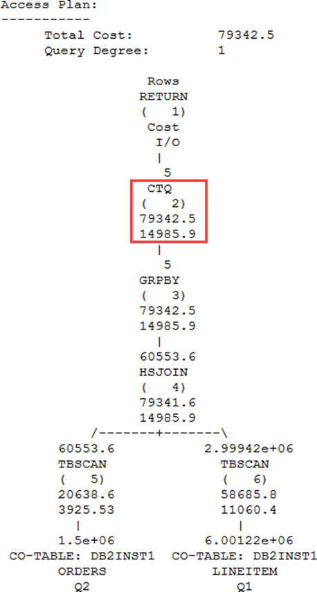
Figure 6-2 An example of a good query execution plan for column-organized tables
Ideally, you want as much of the plan run below the CTQ operator. In good execution plans for column-organized tables, the majority of operators are below the CTQ operator, and only a few rows flow through the CTQ operator (Table 6-2).
Table 6-2 CTQ recommendations
|
Optimal plan
|
Suboptimal plan
|
|
One or few CTQ operators
|
Many CTQs
|
|
Few operators above CTQ
|
Many operators above CTQ
|
|
Operators above CTQ work on few rows
|
Operators above CTQ work on many rows
|
|
Few rows flow through the CTQ
|
Many rows flow through the CTQ
|
In DB2 10.5, the following examples are of some operators that are optimized for column-organized tables:
•Table scan operators
•Hash-based join operators
•Hash-based group by operators
•Hash based unique operators
6.7.2 Time spent on column-organized table processing
Time-spent monitor elements provide information about how the DB2 database manager spends time processing column-organized tables. The time-spent elements are broadly categorized into wait time elements and processing time elements. The columnar-related monitor elements listed in Table 6-3 are added to the time-spent monitoring hierarchy.
Table 6-3 Time spent on queries metrics in the Time area
|
Elements
|
Description
|
|
TOTAL_SECTION_TIME
|
Total column-organized section time monitor element: Represents the total time agents spent performing section execution. The value is given in milliseconds.
|
|
TOTAL_COL_TIME
|
Total column-organized time monitor element: Represents the total elapsed time over all column-organized processing subagents.
|
|
TOTAL_SECTION_PROC_TIME
|
Total column-organized section process time monitor element: Represents the total amount of processing time agents spent performing section execution. Processing time does not include wait time. The value is given in milliseconds.
|
|
TOTAL_COL_PROC_TIME
|
Total column-organized processing time monitor element: Represents the subset of this total elapsed time in which the column-organized processing subagents were not idle on a measured wait time (for example, lock wait or IO).
|
|
TOTAL_COL_EXECUTIONS
|
Total column-organized executions monitor element: Represents the total number of times that data in column-organized tables was accessed during statement execution.
|
You can use these elements, in the context of other “time-spent” monitor elements, to determine how much time was spent, per thread, in performing column-organized data processing. For example, if you want to know what portion of a query was run in column-organized form and what portion was executed in row-organized form, you can compare TOTAL_COL_TIME to TOTAL_SECTION_TIME. A large ratio suggests an optimal execution plan for BLU Acceleration.
Use the query in Example 6-30 to obtain the time spent on column-organized data processing.
Example 6-30 Columnar processing times
SELECT
total_col_time AS TOTAL_COL_TIME,
total_col_executions AS TOTAL_COL_EXECUTIONS,
total_section_time AS TOTAL_SECTION_TIME
FROM
table(mon_get_database(-1));
Your query output should be like the output in Example 6-31.
Example 6-31 Time spent on queries key metrics
TOTAL_COL_TIME TOTAL_COL_EXECUTIONS TOTAL_SECTION_TIME
-------------------- -------------------- --------------------
103679097 121 114185091
1 record(s) selected.
Notice that most of the total time was spent on column-organized data processing (103,656,167 ms out of 114,111,844 ms in the example). This means that our query is using the column-organized data processing advantages of DB2 with BLU Acceleration for the majority of the elapsed processing time.
6.7.3 Observing query performance
The MON_GET_PKG CACHE_STMT table function returns report metrics that relate to key database metrics, such as I/O server efficiency, processing time for authentication, statistics generation, and statement execution. You can use this table function to identify possible problematic static and dynamic SQL statements for both row and columnar query processing.
MON_GET_PKG CACHE_STMT returns a point-in-time view of SQL statements in the database package cache. This has a similar query from Example 6-30 on page 213, except that this is reported per SQL query execution. This allows you to examine the aggregated metrics for a particular SQL statement, and to quickly determine the performance of an executed query. The query in Example 6-32 collects execution times of the statements from the package cache by using the MON_GET_PKG_CACHE_STMT table function.
Example 6-32 Statement execution times
SELECT
varchar(stmt_text,30) AS STATEMENT,
substr(total_cpu_time/num_exec_with_metrics,1,12) AS AVG_CPU_TIME,
total_col_time,
total_section_time,
rows_read,
rows_returned
FROM
table(mon_get_pkg_cache_stmt( NULL, NULL, NULL, -1))
WHERE num_exec_with_metrics <> 0;
Example 6-33 shows output from a Cognos sample workload. It shows that the query section took 76861 ms to execute (TOTAL_SECTION_TIME). Out of the total section time, 73471 ms was spent in column-processing (TOTAL_COL_TIME). That is, about 96% of the time was spent in column-processing and using BLU Acceleration technologies to optimize the query.
Example 6-33 Total column-processing time versus total section time for queries
STATEMENT AVG_CPU_TIME TOTAL_COL_TIME TOTAL_SECTION_TIME
------------------------------ ------------ -------------- ------------------
select "T0"."C0" "C0" , "T0"." 928702 73471 76861
ROWS_READ ROWS_RETURNED
---------- -------------
239968 420
6.7.4 Average number of columns referenced in workload
A new monitor element, TAB_ORGANIZATION, reports information about the organization of data in a table and is returned by the MON_GET_TABLE table function.
BLU Acceleration works best on queries that access only a subset of table columns. This is because of the nature of column-organized table processing. In an environment where majority or all of the workloads tend to access all columns in the tables, traditional row-organized table might achieve more efficient performance rather than scanning different column-organized tables individually.
To determine the average number of columns that a query accesses, you can divide NUM_COLUMNS_REFERENCED by the SECTION_EXEC_WITH_COL_REFERENCES monitor element. If this average is much less than the number of columns in the table, the query is accessing only a small subset of the columns. We can confirm that the workload favors column organization.
Example 6-34 shows how to assess if our workload is columnar in nature.
Example 6-34 Query for assessing if a workload is columnar in nature
SELECT
varchar(b.tabname,25) AS TABNAME,
num_columns_referenced AS NUM_COLUMNS_REFERENCED,
section_exec_with_col_references AS TOTAL_SECS,
cast(num_columns_referenced*1.0/section_exec_with_col_references as decimal(2,1)) AS COL_PER_SEC,
colcount AS COLCOUNT,
card AS ROWCOUNT
FROM
table(mon_get_table('<BLU_SCHEMA>', '<BLU_TABLENAME>',-1)) a,
syscat.tables b
WHERE a.tabschema = b.tabschema
AND a.tabname = b.tabname
AND section_exec_with_col_references > 0
ORDER BY 2 DESC;
Example 6-35 on page 216 shows the result of the query against a series of Cognos Sample Outdoor Warehouse sample analytic workloads. You can see in this test case, that the average number of columns that a particular query accesses in our workload is using the column data organization and we are not scanning all individual column-organized tables for the query.
Example 6-35 Columns per query section versus total column count in tables
TABNAME NUM_COLUMNS_REFERENCED SECTIONS COL_PER_SEC COLCOUNT ROWCOUNT
---------------- ---------------------- -------- ----------- -------- ----------
GO_TIME_DIM 275 38 7.2 73 2930
GO_REGION_DIM 239 34 7.0 66 21
SLS_RTL_DIM 187 32 5.8 88 847
SLS_PRODUCT_DIM 184 28 6.5 14 3000300
SLS_SALES_FACT 184 40 4.6 18 2999547946
Example 6-35 shows that the total column count of each tables (card AS COLCOUNT) is significantly larger than the average number of columns being queried per section (computed COL_PER_SEC). Therefore, we can conclude that this series of executed workload found in the package cache is ideal for BLU Acceleration.
6.7.5 The MONREPORT module
DB2 10.5 also has several modules you can use to generate reports containing a variety of monitoring information.
One of these modules, the MONREPORT module, provides a set of procedures for retrieving a variety of monitoring data and generating text reports. In DB2 10.5, this module was updated to include columnar monitor elements.
In particular, the procedures that were updated are as follows:
•MONREPORT.CONNECTION: This procedure outputs a summary report based on connection information from MON_GET_CONNECTION.
•MONREPORT.DBSUMMARY: This procedure outputs a summary report, based on MON_GET_SERVICE_SUBCLASS, MON_GET_CONNECTION and MON_GET_WORKLOAD.
You use the following DB2 commands to call these procedures:
db2 call monreport.connection;
db2 call monreport.dbsummary;
The report contains a good amount of monitor information for the entire database and also key performance indicators for each connection, workload, service class, and database member.
For a sample output of the database summary report from monreport, see A.1, “Sample Monreport output” on page 412.
..................Content has been hidden....................
You can't read the all page of ebook, please click here login for view all page.