

DB2 with BLU Acceleration and SAP integration
This chapter contains information about the integration of DB2 for Linux, UNIX, and Windows (DB2) with BLU Acceleration into SAP Business Warehouse (SAP BW) and into the SAP BW near-line storage solution (NLS). We list the SAP releases in which BLU Acceleration is supported and the SAP and DB2 software prerequisites.
We discuss ABAP Dictionary integration of BLU Acceleration and how to monitor the DB2 columnar data engine in the SAP DBA Cockpit, as well as the usage of BLU Acceleration in SAP BW in detail. We explain which SAP BW objects BLU Acceleration can be used with, how to create new SAP BW objects that use column-organized tables, and how to convert existing SAP BW objects from row-organized to column-organized tables.
We provide information about installing SAP BW systems on DB2 10.5 and about the handling of BLU Acceleration in migrations of SAP BW systems to DB2 10.5. Results from IBM internal lab tests give a description of performance and compression benefits that you can achieve with BLU Acceleration in SAP BW systems. We also provide preferred practices and suggestions for DB2 parameter settings when BLU Acceleration is used in SAP BW.
We explain is the usage of BLU Acceleration in SAP’s near-line storage solution on DB2 in detail, showing for which SAP BW objects in the near-line storage archive BLU Acceleration can be used, and how to create new data archiving processes (DAPs) that use column-organized tables in the near-line storage database.
Finally, we demonstrate installing an NLS database on DB2 10.5 and the preferred practices for DB2 parameter settings when using BLU Acceleration in SAP BW NLS systems.
The following topics are covered:
8.1 Introduction to SAP Business Warehouse (BW)
This section briefly describes the elements of the SAP BW information model. The information in this section is an excerpt from the SAP Help Portal for SAP BW (Technology → SAP NetWeaver Platform → 7.3 → Modeling → Enterprise Data Warehouse Layer)1.
SAP BW is part of the SAP NetWeaver platform. Key capabilities of SAP BW are the buildup and management of enterprise, and departmental data warehouses for business planning, enterprise reporting and analysis. SAP BW can extract master data and transactional data from various data sources and store it in the data warehouse. This data flow is defined by the SAP BW information model (Figure 8-1).
Furthermore, SAP BW is the basis technology for several other SAP products such as SAP Strategic Enterprise Management (SAP SEM), SAP Business Planning and Consolidation (SAP BPC).

Figure 8-1 SAP BW information model
8.1.1 Persistent Staging Area (PSA)
Usually, data extracted from source systems is first stored directly in the Persistent Staging Area (PSA) as it was received from the source system. PSA is the inbound storage area in SAP BW for data from the source systems. PSA is implemented with one transparent database table per data source.
8.1.2 InfoObjects
InfoObjects are the smallest information units in SAP BW. They can be divided into three groups:
•Sets of characteristics, modeled as master data references, form entities. Such a reference remains unchanged, even if the corresponding value (attribute) is changed. Additional time characteristics are used to model the state of an entity over the course of time.
•Numerical attributes of entities are modeled as key figures. They are used to describe their state at a certain point of time.
•Units and other technical characteristics are used for processing and transformation purposes.
InfoObjects for characteristics consist of several database tables. They contain information about time-independent and time-dependent attributes, hierarchies, and texts in the languages needed. The central table for characteristics is the surrogate identifiers (SIDs) table that associates the characteristics with an integer called SID. That is used as foreign key to the characteristic in the dimension tables of InfoCubes.
8.1.3 DataStore Objects (DSOs)
DSOs store consolidated and cleansed transactional or master data on an atomic level. SAP BW offers three types of DSOs:
•Standard
•Write-optimized
•Transactional
Write-optimized and transactional DSOs consist of one database table that is called the DSO active table.
Standard DSOs consist of three database tables:
•The activation queue table
•The active table
•The change log table
The data that is loaded into standard DSOs is first stored in the activation queue table. The data in the activation queue table is not visible in the data warehouse unless it has been processed by a complex procedure that is called DSO data activation. Data activation merges the data into the active table and writes before and after images of the data into the change log table. The change log table can be used to roll back activated data if the data is not correct or other issues occur.
8.1.4 InfoCubes
InfoCubes are used for multidimensional data modeling according to the star schema. There are several types of InfoCubes. Two of them are introduced in this section:
Standard InfoCubes
SAP BW uses the enhanced star schema as shown in Figure 8-2 on page 250, which is partly normalized. An InfoCube consists of two fact tables, F and E. They contain recently loaded and already compressed data. To provide a single point of access, a UNION ALL view is defined on these two tables. The fact tables contain the key figures and foreign keys to up to 16 dimension tables. The dimension tables contain an integer number DIMID as primary key and the SIDs to the characteristics that belong to the dimension.
The F fact table is used for staging new data into the InfoCube. Each record contains the ID of the package with which the record was loaded. To accelerate the load process, data from one package is loaded to the F fact table in blocks. Although a certain combination of characteristics will be unique in each block, there can be duplicates in different blocks and packages. By the assignment of loaded data to packages, incorrect or mistakenly loaded data can be deleted easily as long as it resides in the F fact table.
The process of bringing the data from the F fact table to the E fact table is called InfoCube compression. In the course of this, the relation to the package is removed and multiple occurrences of characteristic combinations are condensed. Thus the F fact table contains only unique combinations of characteristics. Compressed packages are deleted from the F fact table after compression is completed.

Figure 8-2 SAP BW extended star schema
InfoCube query processing
The SAP BW OLAP processor maps the query to the underlying InfoProvider. It processes reporting queries and translates them into a series of SQL statements that are sent to the database. Depending on the query, the OLAP processor might run additional complex processing to combine the results of the SQL queries into the final result that is sent back to the user.
A typical BW InfoCube query involves joins between the fact, dimension, and master data tables, as shown in Example 8-1.
Example 8-1 Sample SAP BW Query
-- Projected columns
SELECT "X1"."S__0INDUSTRY" AS "S____1272"
, "DU"."SID_0BASE_UOM" AS "S____1277"
, "DU"."SID_0STAT_CURR" AS "S____1278"
, "X1"."S__0COUNTRY" AS "S____1270"
, SUM ( "F"."CRMEM_CST" ) AS "Z____1279"
, SUM ( "F"."CRMEM_QTY" ) AS "Z____1280"
, SUM ( "F"."CRMEM_VAL" ) AS "Z____1281"
, COUNT( * ) AS "Z____031"
-- F fact table
FROM "/BI0/F0SD_C01" "F“
-- Dimension tables
JOIN "/BI0/D0SD_C01U" "DU" ON "F“ ."KEY_0SD_C01U" = "DU"."DIMID“
JOIN "/BI0/D0SD_C01T" "DT" ON "F“ ."KEY_0SD_C01T" = "DT"."DIMID“
JOIN "/BI0/D0SD_C01P" "DP" ON "F“ ."KEY_0SD_C01P" = "DP"."DIMID“
JOIN "/BI0/D0SD_C013" "D3" ON "F“ ."KEY_0SD_C013" = "D3"."DIMID“
JOIN "/BI0/D0SD_C011" "D1" ON "F“ ."KEY_0SD_C011" = "D1"."DIMID"
-- Master data attribute table
JOIN "/BI0/XCUSTOMER" "X1" ON "D1"."SID_0SOLD_TO" = "X1"."SID“
-- Predicates
WHERE ( ( ( ( "DT"."SID_0CALMONTH" IN ( 201001, 201101, 201201,
201301, 201401 ) ) )
AND ( ( "DP"."SID_0CHNGID" = 0 ) )
AND ( ( "D3"."SID_0DISTR_CHAN" IN ( 9, 7, 5, 3 ) ) )
AND ( ( "D3"."SID_0DIVISION" IN ( 3, 5, 7, 9 ) ) )
AND ( ( "DP"."SID_0RECORDTP" = 0 ) )
AND ( ( "DP"."SID_0REQUID" <= 536 ) )
AND ( ( "X1"."S__0INDUSTRY" IN ( 2, 4, 6, 9 ) ) )
) )
AND "X1"."OBJVERS" = 'A‘
-- Aggregation
GROUP BY "X1"."S__0INDUSTRY"
, "DU"."SID_0BASE_UOM"
, "DU"."SID_0STAT_CURR"
, "X1"."S__0COUNTRY"
;
In this case, the fact table, the F fact table /BI0/F0SD_C01, is joined to several dimension tables, /BI0/D0SD_C01x, and the table of dimension 1, /BI0/D0SD_C011, is joined to a master data attribute table, /BI0/XCUSTOMER, to extract information about customers in certain industries.
SAP BW query processing might involve SQL queries that generate intermediate temporary results that are stored in database tables. Consecutive SQL queries join these tables to the InfoCube tables. The following examples make use of such tables:
•Evaluation of master data hierarchies
•Storage of a large number of master data SIDs, considered as too large for an IN-list in the SQL query
•Pre-materialization of joins between a dimension table and master data tables when the SAP BW query involves a large number of tables to be joined
Flat InfoCubes
Flat InfoCubes are similar to standard InfoCubes. However, they use a simplified schema as shown in Figure 8-3. The E fact table and all dimension tables other than the package dimension table are eliminated from the original schema. The SIDs of the characteristics are directly stored in the fact table. For databases other than SAP HANA, flat InfoCubes are only available in SAP BW 7.40 Support Package 8 and higher.

Figure 8-3 Flat InfoCube
From the storage point of view, one aspect is that this denormalization increases the redundancy of data in the fact table significantly; the other aspect is that two columns per dimension are dropped which were required for the foreign key relation. Furthermore, the compression algorithm of DB2 with BLU Acceleration can reach high compression rates on redundant data. Thus, in most cases, the impact of the denormalization on the total storage consumption is low.
The number of columns of the fact table is considerably increased by the denormalization. Using BLU Acceleration this does not affect the query performance, because only those columns are read, which are actually required.
You can run InfoCube compression on flat InfoCubes. Compressed and uncompressed data are stored in the same fact table (the F fact table).
Flat InfoCubes have the following advantages:
•Reporting queries might run faster because less tables have to be joined.
•Data propagation into flat InfoCubes might run faster because the dimension tables do not need to be maintained. This is especially true in cases where some dimension tables are large.
•Administration and modelling simplified because line items do not have to be handled separately and the logical assignment of characteristics to dimensions can be changed without any effort.
In SAP BW, the following restrictions apply to flat InfoCubes:
•Flat InfoCubes cannot be stored in the SAP Business Warehouse Accelerator (BWA).
•Aggregates cannot be created for flat InfoCubes.
Aggregates and SAP Business Warehouse Accelerator
To increase speed of reporting, SAP BW allows the creation of aggregates for non flat InfoCubes. Aggregates contain pre-calculated aggregated data from the InfoCubes. They are comparable to materialized query tables but are completely managed by SAP BW. The SAP BW OLAP processor decides when to route a query to an SAP BW aggregate. The creation and maintenance of aggregates is a complex and time-consuming task that takes a large portion of the extract, transform, and load (ETL) processing time.
SAP offers the SAP Business Warehouse Accelerator (SAP BW Accelerator) for speeding up reporting performance without the need to create aggregates. SAP BW Accelerator runs on a separate hardware and does not support flat InfoCubes. InfoCubes and master data can be replicated into SAP BW Accelerator. Starting with SAP BW 7.30, InfoCubes that reside only in SAP BW Accelerator can be created. When InfoCubes and master data are replicated, the SAP BW Accelerator data must be updated when new data is loaded into SAP BW. This creates ETL processing overhead.
8.1.5 BLU Acceleration benefits for SAP BW
Creating column-organized database tables for SAP BW objects provides the following benefits:
•Reporting queries run faster on column-organized tables. Performance improvements vary and depend on the particular query, but results from customer proof of concepts show that a factor greater than ten can be achieved in many cases.
•These performance improvements can be achieved with little or no database tuning effort. Table statistics are collected automatically. Table reorganization, the creation of indexes for specific queries, statistical views, or database hints are usually not needed.
•Because of the much faster query performance, aggregates might not be required any more, or at least the number of aggregates can be reduced significantly. Even the SAP BW Accelerator might become obsolete. This greatly improves the ETL processing time because aggregate rollup and updating the SAP BW Accelerator data is no longer required.
•Except for primary key and unique constraints, column-organized tables have no indexes. Thus, during ETL processing, hardly any time needs to be spent on index maintenance and index logging. This significantly reduces the SAP ETL processing time and the active log space consumption, especially for ETL operations such as InfoCube data propagation and compression. Also data deletion might run much faster, especially when MDC rollout is not applicable on a certain object.
•The compression ratio of column-organized tables is much higher than the ratio achieved with adaptive compression on row-organized tables. In addition, space requirements for indexes are drastically reduced.
•Modelling of InfoCubes is simplified by the use of flat InfoCubes because the logical assignment of characteristics to dimensions can be changed without any effort.
8.2 Prerequisites and restrictions for using BLU Acceleration in SAP BW
This section discusses the following topics:
•Important SAP documentation and SAP Notes that you should read
•Prerequisites and restrictions for using DB2 BLU Acceleration in SAP BW
•Required SAP Support Packages and DBSL kernel patches
•Required SAP Kernel parameter settings
8.2.1 Important SAP documentation and SAP notes
Before you use BLU Acceleration in SAP BW and SAP NLS on DB2, see the available SAP documentation:
•Database administration guide:
Select <Your SAP NetWeaver Main Release> → Operations → Database-Specific Guides.
The name of the guide is: SAP Business Warehouse on IBM DB2 for Linux, UNIX, and Windows: Administration Tasks.
•How-to guide:
Select <Your SAP NetWeaver Main Release> → Operations → Database-Specific Guides
The name of the guide is: Enabling SAP Business Warehouse Systems to Use IBM DB2 for Linux, UNIX, and Windows as Near-Line Storage (NLS).
•Database upgrade guide:
Database Upgrade Guide Upgrading to Version 10.5 of IBM DB2 for Linux, UNIX, and Windows2:
Database Upgrades → DB2 UDB → Upgrade to Version 10.5 of IBM DB2 for LUW
SAP Notes3 with general information about the enablement of DB2 10.5 with BLU Acceleration are listed in Table 8-1.
Table 8-1 SAP Notes regarding the enablement of BLU Acceleration in SAP Applications
|
SAP Note
|
Description
|
|
1555903
|
Gives an overview on the supported DB2 features.
|
|
1851853
|
Describes the SAP software prerequisites for using DB2 10.5 in general for SAP applications. The note also provides an overview of the new DB2 10.5 features that are relevant for SAP, including BLU Acceleration.
|
|
1851832
|
Contains a section about DB2 parameter settings for BLU Acceleration.
|
|
1819734
|
Describes prerequisites and restrictions for using BLU Acceleration in the SAP environment (includes corrections).
|
The SAP Notes in Table 8-2 contain corrections and advises that you must install to enable BLU Acceleration for the supported SAP BW based applications. You can install these SAP Notes using SAP transaction SNOTE.
Table 8-2 SAP Notes regarding BLU Acceleration of SAP BW based Applications
|
SAP Note
|
Description
|
|
1889656
|
Contains mandatory fixes you must apply before you use BLU Acceleration in SAP BW. With the Support Packages installed, which are listed in 8.2.2, “Prerequisites and restrictions for using DB2 BLU Acceleration” on page 258, this is only necessary for SAP BW 7.0 Support Package 32.
|
|
1825340
|
Describes prerequisites and the procedure for enabling BLU Acceleration in SAP BW.
|
|
2034090
|
Contains recommendations and best practices for SAP BW objects with BLU Acceleration created on DB2 10.5 FP3aSAP or earlier.
|
|
1911087
|
Contains an advise regarding a DBSL patch.
|
|
1834310
|
Describes how to enable BLU Acceleration for SAP’s near-line storage solution on DB2 (includes corrections).
|
|
1957946
|
Describes potential issues with column-organized InfoCubes. This note is only relevant if you use DB2 10.5 FP3aSAP. If you often make structural changes to InfoCubes, for example, by adding key figures or by adding or changing dimensions, you should upgrade to DB2 Cancun Release 10.5.0.4.
|
The list of SAP Notes listed in Table 8-3 contain further improvements and code fixes. They should be installed as well to achieve the best functionality.
Table 8-3 SAP Notes with further improvements and fixes
|
SAP Note
|
Description
|
|
1964464
|
Contains specific fixes for the conversion report from row-organized to column-organized tables. This is needed if you want to convert existing InfoCubes to BLU on DB2 10.5 FP3aSAP or earlier.
|
|
1996587 2022487
|
Contain code fixes for the InfoCube compression of the accelerated InfoCubes with BLU Acceleration.
|
|
1979563
|
Contains a fix for eliminating mistakenly created warning messages in the SAP work process trace files.
|
|
2019648
|
Handles issues that might occur when you transport a BLU InfoCube to a system that does not use automatic storage or does not use reclaimable storage tablespaces.
|
|
2020190
|
Contains corrections for BLU InfoCubes with dimensions that contain more than 15 characteristics
|
Starting with DB2 Cancun Release 10.5.0.4, several additional features have been added, which can be enabled by applying the SAP Notes in Table 8-4.
Table 8-4 SAP Notes for DB2 Cancun Release 10.5.0.4 specific features
|
SAP Note
|
Description
|
|
1997314
|
Required to use BLU Acceleration for DataStore Objects, InfoObjects, and PSA tables. This is only supported as of DB2 Cancun Release 10.5.0.4.
|
|
2038632
|
Required for using flat InfoCubes in SAP BW 7.40 Support Package 8 or higher. This is only supported as of DB2 Cancun Release 10.5.0.4.
|
|
1947559 1969500
|
These notes are required for SAP system migrations. They enable the generation of BW object tables directly as BLU tables without the need to run conversions to BLU in the migration target system later. This is only supported when your DB2 target system is set up on DB2 Cancun Release 10.5.0.4 or higher.
|
8.2.2 Prerequisites and restrictions for using DB2 BLU Acceleration
BLU Acceleration is currently only supported in SAP BW, SAP Strategic Enterprise Management (SAP SEM), and SAP NLS on DB2. BLU Acceleration is not supported in other SAP applications, including applications that are based on SAP BW, such as SAP Supply Chain Management (SAP SCM). The latest list of supported products can be found in SAP Note 1819734.
The following additional restrictions for your DB2 database apply:
•You need at least DB2 10.5 Fix Pack 3aSAP. The preferred version is DB2 Cancun Release 10.5.0.4 or later, which provides additional significant optimizations and performance improvements for SAP and enables the BLU implementation for DSOs, InfoObjects, and PSA tables.
•BLU DSOs, InfoObjects, and PSA tables are only supported as of DB2 Cancun Release 10.5.0.4 (see SAP Note 1997314). All InfoObject types except for key figures (for which no database tables are created) are supported.
•Flat InfoCubes are only supported as of DB2 Cancun Release 10.5.0.4 and SAP BW 7.40 Support Package 8.
•Your database server runs on platform that supports BLU Acceleration. At the time of writing these are AIX or Linux on the X86_64 platform.
•Your database uses Unicode.
•You do not use DB2 pureScale and do not use the DB2 Database Partitioning Feature (DPF).
•If you use DB2 10.5 Fix Pack 3aSAP you do not use HADR. This restriction does not exist any more in DB2 Cancun Release 10.5.0.4 release.
•Your database is set up with DB2 automatic storage.
•You provide reclaimable storage tablespaces for the BLU tables.
8.2.3 Required Support Packages and SAP DBSL Patches
SAP BW 7.0 and later are supported. The lowest preferred Support Packages for each SAP BW release are shown in Table 8-5. With DB2 Cancun Release 10.5.0.4 and these Support Packages and additional SAP notes that have to be installed on top, BLU Acceleration for InfoCubes, DataStore objects, InfoObjects, PSA tables, and BW temporary tables is available. Furthermore, it is possible to directly create column-organized tables in SAP BW system migrations to DB2 10.5.
Table 8-5 Supported SAP BW releases and Support Packages
|
SAP NetWeaver release
|
SAP BASIS Support Package
|
SAP BW Support
Package |
|
7.0
|
30
|
32
|
|
7.01
|
15
|
15
|
|
7.02
|
15
|
15
|
|
7.11
|
13
|
13
|
|
7.30
|
11
|
11
|
|
7.31/7.03
|
11
|
11
|
|
7.40
|
6
|
6
|
These support packages contain ABAP code that is specific to DB2 in the SAP Basis and SAP BW components that enable the use of BLU Acceleration and extensions to the DBA Cockpit for monitoring and administering SAP DB2 databases. They are prerequisites for using BLU Acceleration in SAP BW. For more details, see SAP Notes 1819734 and 1825340.
We suggest that you also install the latest available SAP kernel patches and SAP Database Shared Library (DBSL). The minimum required DBSL patch level for using DB2 Cancun Release 10.5.0.4 with BLU Acceleration in SAP BW and SAP’s near-line storage solution on DB2 can be found in SAP Note 2056603. These patch levels are higher than the levels listed in the SAP database upgrade guide: Upgrading to Version 10.5 of IBM DB2 for Linux, UNIX, and Windows.
8.2.4 Required SAP kernel parameter settings
As of DB2 Cancun Release 10.5.0.4 and SAP BW support InfoObjects, the following SAP kernel parameters are required:
•dbs/db6/dbsl_ur_to_cc=*
This parameter sets the default DB2 isolation level that is used in the SAP system to Currently Committed. This applies to all SQL statements that otherwise run with isolation level UR (uncommitted read) by default. This parameter is needed to avoid potential data inconsistencies during the update of existing master data and insertion of new master data in the SAP BW system.
•dbs/db6/deny_cde_field_extension=1
This parameter prevents operations in the SAP BW system that extend the length of a VARCHAR column in a column-organized table. Extending the length of a VARCHAR column in a column-organized table is not supported in DB2 10.5 and causes SQL error SQL1667N. (The operation failed because the operation is not supported with the type of the specified table. Specified table: <tabschema>.<tabname>. Table type: “ORGANIZE BY COLUMN”. Operation: “ALTER TABLE”. SQLSTATE=42858). When the SAP profile parameter is set, the SAP ABAP Dictionary triggers a table conversion if extending the length of a VARCHAR column in a column-organized table is requested.
8.3 BLU Acceleration support in the ABAP Dictionary
In the ABAP Dictionary, storage parameters are used to identify column-organized tables. The property, including the column-organized table, can be retrieved from the database and displayed in the “Storage Parameter” window of the SAP data dictionary.
In the example in Figure 8-4, the /BIC/FICBLU01 table is a column-organized table. Use the following steps to look up the storage parameters of the transaction table SE11:
1. Enter the table name in the Database table field and select Display.

Figure 8-4 ABAP Dictionary initial window
2. In the “Dictionary: Display” table window, select Utilities → Database Object → Database Utility from the menu (Figure 8-5).

Figure 8-5 ABAP Dictionary: retrieval of table properties
3. In the “ABAP Dictionary: Utility for Database Tables” window, select Storage Parameters, as shown in Figure 8-6.

Figure 8-6 ABAP Dictionary: retrieval of table database storage parameters
The “Storage parameters: (display and maintain)” window (Figure 8-7) shows the table properties that are retrieved from the DB2 system catalog. The last entry with the OPTIONS label is ORGANIZE BY COLUMN, which shows that the table is organized column-oriented.

Figure 8-7 Table storage parameters of a column-organized SAP BW F fact table
|
Notes:
•Although BLU Acceleration does not require DPF for parallel query processing, DB2 accepts the specification of a distribution key. In SAP BW, distribution keys are always created for InfoCube fact, DSO, and PSA tables.
SAP uses the term PARTITIONING KEY for distribution keys in the ABAP Dictionary.
•SAP NetWeaver 7.40 introduces an option in the ABAP Dictionary to specify whether a table should be created in Column Store or in Row Store. This option does not trigger creation of column-organized tables in DB2.
|
8.4 BLU Acceleration support in the DBA Cockpit
The DBA Cockpit has been enhanced with the DB2 monitoring elements for column-organized tables.
The DBA Cockpit extensions for BLU Acceleration are available in the SAP NetWeaver releases and Support Packages listed in the second column of Table 8-6. With these Support Packages, time spent analysis, the BLU Acceleration buffer pool, and I/O metrics are only available in the Web Dynpro user interface. When you upgrade to the Support Packages listed in column three, these metrics are included in the SAP GUI user interface.
Table 8-6 Availability of DBA Cockpit enhancements for BLU Acceleration in the SAP Web Dynpro and SAP GUI user interfaces
|
SAP NetWeaver release
|
SAP BASIS Support Package for BLU Acceleration metrics in Web Dynpro
|
SAP BASIS Support Package for BLU Acceleration metrics in SAP GUI
|
|
7.02
|
14
|
15
|
|
7.30
|
10
|
11
|
|
7.31
|
9
|
11
|
|
7.40
|
4
|
6
|
We suggest that you also implement SAP Note 1456402. This SAP Note contains a patch collection for the DBA Cockpit that is updated regularly. You can install the most recent DBA Cockpit patches by reinstalling the patch collection SAP Note. When you reinstall the SAP Note, only the delta between your current state and the most recently available patches is installed.
When you monitor your SAP systems using SAP Solution Manager, you need SAP Solution Manager 7.1 Support Package 11 to get the BLU Acceleration metrics.
For SAP BW 7.0 and SAP BW 7.01, a compatibility patch for DB2 10.5 is available in the Support Packages that are required for using BLU Acceleration in SAP BW. This patch handles only changes in the DB2 monitoring interfaces that are used in the DBA Cockpit. It does not provide any extra metrics for BLU Acceleration in the DBA Cockpit of SAP NetWeaver 7.0 and 7.01.
With the DBA Cockpit enhancements for BLU Acceleration, you can obtain the following information:
•Individual table information, including whether the table is column-organized
•Database information, including the databases that contain column-organized tables
•Columnar data processing information as part of time spent analysis
•Buffer pool hit ratio, buffer pool read and write activity, and prefetcher activity for the whole database, buffer pools, table spaces, and applications
In the following sections, we provide examples of BLU Acceleration monitoring using the DBA Cockpit. The windows in the figures are from an SAP BW 7.40 system running on Support Package stack 5.
8.4.1 Checking whether individual tables in SAP database are column-organized
In the DBACOCKPIT transaction, choose Space → Single Table Analysis in the navigation frame (Figure 8-8). Enter the table name in the Name field of the Space: Table and Indexes Details window and press Enter. You find the table organization in the Table Organization field on the System Catalog tab.

Figure 8-8 DBA Cockpit: properties of a single table
8.4.2 Checking if SAP database contains column-organized tables
In the DBACOCKPIT transaction, choose Configuration → Parameter Check in the navigation frame (Figure 8-9). On the Check Environment tab in the Parameter Check window, find the System Characteristics panel. If the CDE attribute has the value YES, the database contains column-organized tables.

Figure 8-9 DBA Cockpit: DB2 configuration parameter check window
8.4.3 Monitoring columnar data processing time in the SAP database
Time spent analysis was originally only available in the Web Dynpro user interface. With the service packs listed Table 8-6 on page 265 it is available in SAP GUI as well. The configuration of the Web Dynpro user interface is described in SAP Note 1245200.
Choose Performance → Time Spent Analysis in the navigation frame of the DBA Cockpit. A window similar to the one shown in Figure 8-10 opens. Enter the time frame for which you want to retrieve the information. The window is updated and shows how much time DB2 spent in various activities, including the columnar processing time in the selected time frame.

Figure 8-10 DBA Cockpit: Analysis of time spent in DB2
8.4.4 Monitoring columnar processing-related prefetcher and buffer pool activity in the SAP database
You can monitor buffer pool and prefetcher activity at database, workload, table space, and application level.
Choose Performance → (Snapshots → )4 Database in the DBA Cockpit. Select the time frame for which you want to display the information. On the “Buffer Pool” tab in the “History Details” area (Figure 8-11), you see the logical and physical reads, the physical writes, synchronous reads and writes, and temporary logical and physical reads on column-organized tables in the “Columnar” section. In the “Buffer Quality” section, you see the buffer pool hit ratio for column-organized tables.

Figure 8-11 DBA Cockpit: Buffer pool metrics
As shown in Figure 8-12, when you switch to the “Asynchronous I/O” tab, you find separate counters for column-organized tables in these sections:
•Prefetcher I/O
•Total No. of Skipped Prefetch Pages
•Skipped Prefetch Pages Loaded by Agents in UOW sections.
For example, the “Prefetcher I/O” section shows “Columnar Prefetch Requests”, which is the number of column-organized prefetch requests successfully added to the prefetch queue. This corresponds to the pool_queued_async_col_reqs DB2 monitoring element.

Figure 8-12 DBA Cockpit: Asynchronous I/O metrics
To retrieve the buffer pool and prefetcher information for individual table spaces, buffer pools, and for the current unit of work of an application, choose Performance → (Snapshots → ) Tablespaces, Bufferpools, or Applications in the DBA Cockpit navigation frame.
8.5 BLU Acceleration support in SAP BW
You can do the following operations in SAP BW:
•In the SAP Data Warehousing Workbench, you can create InfoCubes, DSOs, InfoObjects, and PSA tables as column-organized tables in the database. The following list indicates the supported BW object types:
– Basic cumulative InfoCubes
– Basic non-cumulative InfoCubes
– Multi-Cubes with underlying column-organized basic InfoCubes
– Multi-Provider which consolidate several InfoProvider
– In SAP BW 7.30 and higher, semantically partitioned InfoCubes
– As of DB2 Cancun Release 10.5.0.4 BLU Acceleration is also supported for the following BW objects:
• Standard DSOs
• Write-optimized DSOs
• InfoObjects (characteristics, time characteristics, units), through a new RSADMIN parameter
• PSA tables, through a new RSADMIN parameter
You cannot create column-organized real-time InfoCubes and transactional DSOs.
•As of SAP BW 7.40 Support Package 8 and DB2 Cancun Release 10.5.0.4, you can work with flat InfoCubes. Flat InfoCubes have a simplified star schema with only one fact table and no dimension tables except for the package dimension table. You can create flat InfoCubes and you can convert existing standard InfoCubes to flat InfoCubes (see 8.5.2, “Flat InfoCubes in SAP BW 7.40” on page 297).
•DB6CONV is enhanced with the option to convert BW objects (InfoCubes, DSOs, InfoObjects, and PSA tables) from row-organized to column-organized tables. You can convert selected BW objects or all BW objects in your system (see 8.6, “Conversion of SAP BW objects to column-organized tables” on page 350). Thus, the SAP_CDE_CONVERSION report is discontinued with DB2 Cancun Release 10.5.0.4.
•You can set an SAP BW RSADMIN configuration parameter that causes new InfoObject SID and attribute SID tables to be created as column-organized tables.
•You can set an SAP BW RSADMIN configuration parameter that causes new PSA tables to be created as column-organized tables.
•You can set an SAP BW RSADMIN configuration parameter that causes new SAP BW temporary tables to be created as column-organized tables.
In this section, we explain in detail how to perform these operations.
8.5.1 Column-organized standard InfoCubes in SAP BW
This section shows how to create a new standard InfoCube that uses column-organized tables in the Data Warehousing Workbench of SAP BW. We illustrate the procedure with an example in an SAP BW 7.40 system in which the BI DataMart Benchmark InfoCubes have been installed (InfoArea BI Benchmark). The example works in exactly the same way in the other SAP BW releases in which BLU Acceleration is supported.
Follow these steps to create a new InfoCube that uses column-organized tables in the Data Warehousing Workbench of SAP BW:
1. Call transaction RSA1 to get to the Data Warehousing Workbench and create the InfoArea BLU Acceleration Example InfoArea (Figure 8-13).
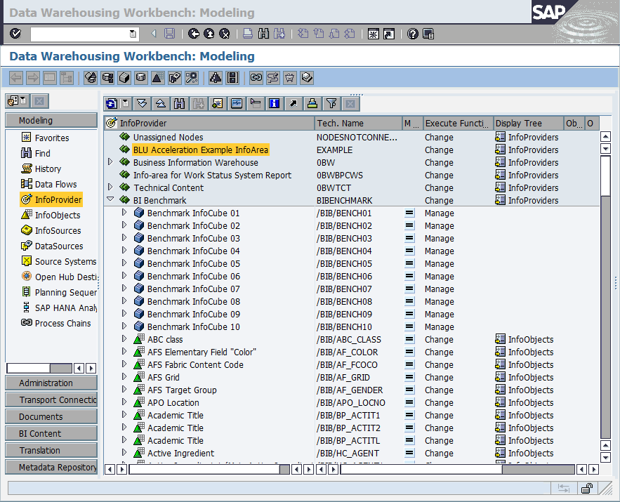
Figure 8-13 SAP Data Warehousing Workbench main window
2. In BI Benchmark, select Benchmark InfoCube 01 (technical name is /BIB/BENCH01), and choose Copy from the context menu (Figure 8-14).

Figure 8-14 SAP Data Warehousing Workbench: Copying an InfoCube
3. In the Edit InfoCube window, enter BLUCUBE1 as the technical name, BLU Demo InfoCube 1 as the description, and select EXAMPLE (BLU Acceleration Example InfoArea) as the InfoArea. Click the Create icon (Figure 8-15).
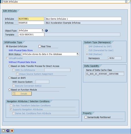
Figure 8-15 SAP Data Warehousing Workbench: Editing InfoCube window
4. The Edit InfoCube window in the Data Warehousing Workbench opens. From the menu, choose Extras → DB Performance → Clustering (Figure 8-16).

Figure 8-16 SAP Data Warehousing Workbench: Specifying DB2-specific properties
5. In the Selection of Clustering dialog window, select Column-Organized and then click the check mark icon to continue (Figure 8-17).

Figure 8-17 SAP Data Warehousing Workbench: Select column-organized tables
6. Save and activate the InfoCube.
7. Inspect the tables:
In transaction RSA1, you can inspect the tables of an InfoCube by choosing Extras → Information (logs/status) from the menu (Figure 8-18).
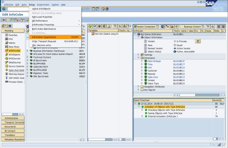
Figure 8-18 SAP Data Warehousing Workbench: Accessing protocol and status information
In the Info Selection dialog window, click Dictionary/DB Status (Figure 8-19).
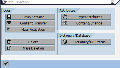
Figure 8-19 Accessing ABAP Dictionary for the tables of an InfoCube
The “Status Information” window displays the tables of the InfoCube. To look up the storage parameters for the table, double-click a table to get to the ABAP Dictionary information for the table (Figure 8-20).

Figure 8-20 ABAP Dictionary information for a InfoCube table
When you work with BLU Acceleration InfoCubes, consider the following information:
•When you copy an existing InfoCube, the target InfoCube inherits the clustering and table organization settings of the source InfoCube. You can change the settings of the target InfoCube in the “Selection of Clustering” window in the Data Warehousing Workbench before you activate the target InfoCube.
•You might no longer need aggregates when you work with BLU Acceleration InfoCubes because the query performance on the basic InfoCubes is fast enough. However, you can create aggregates for BLU Acceleration InfoCubes just as for row-organized InfoCubes if needed. The tables for any aggregates of BLU Acceleration InfoCubes are also created as column-organized tables.
•When you install InfoCubes from SAP BI Content, they are created with the default clustering settings for DB2, which is index clustering. If you want to create BLU Acceleration InfoCubes, you must change the clustering settings in the Data Warehousing Workbench after you install the InfoCubes, and then reactivate the InfoCubes.
•When you transport an InfoCube from your development system into the production system, the behavior is as follows:
– If the InfoCube already exists in the production system and contains data, the current clustering settings and table organization are preserved.
– If the InfoCube does not yet exist in the production system or does not contain any data, the clustering and table organization settings from the development system are used. If the tables exist, they are dropped and re-created.
•When you create a semantically partitioned InfoCube, the clustering settings that you select for the semantically partitioned InfoCube are propagated to the partitions of the InfoCube. Therefore, when you choose to create column-organized tables, the tables of all partitions of the semantically partitioned InfoCube are created automatically as column-organized.
Table layout of column-organized InfoCubes
This section shows the differences in the layout of row-organized and column-organized InfoCube tables.
For comparison, we also create ROWCUBE1, a row-organized InfoCube. Here we use multidimensional clustering (MDC) on the package dimension key column of the InfoCube F fact table and on the time characteristic calendar month on the InfoCube F and E fact tables:
1. You select these clustering settings for the row-organized InfoCube in SAP BW by choosing Multi-Dimensional Clustering in the “Selection of Clustering” dialog window (Figure 8-21).
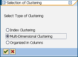
Figure 8-21 SAP Data Warehousing Workbench: Creating a sample row-organized InfoCube
2. Then make selections in the “Multi-Dimensional Clustering” dialog window (Figure 8-22).
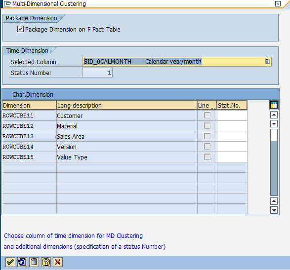
Figure 8-22 Specification of multi-dimensional clustering for the sample row-organized InfoCube
3. Save and activate the InfoCube. After that, the tables listed in Figure 8-23 exist for ROWCUBE1 InfoCube.

Figure 8-23 Tables of the sample row-organized InfoCube
Comparison of the F fact tables
You can use the DB2 db2look tool to extract the DDL for the two fact tables:
db2look -d D01 -a -e -t "/BIC/FBLUCUBE1"
Example 8-2 shows the DDL of the table.
Example 8-2 DDL of column-organized F fact table
CREATE TABLE "SAPD01 "."/BIC/FBLUCUBE1" (
"KEY_BLUCUBE1P" INTEGER NOT NULL WITH DEFAULT 0 ,
"KEY_BLUCUBE1T" INTEGER NOT NULL WITH DEFAULT 0 ,
"KEY_BLUCUBE1U" INTEGER NOT NULL WITH DEFAULT 0 ,
"KEY_BLUCUBE11" INTEGER NOT NULL WITH DEFAULT 0 ,
"KEY_BLUCUBE12" INTEGER NOT NULL WITH DEFAULT 0 ,
"KEY_BLUCUBE13" INTEGER NOT NULL WITH DEFAULT 0 ,
"KEY_BLUCUBE14" INTEGER NOT NULL WITH DEFAULT 0 ,
"KEY_BLUCUBE15" INTEGER NOT NULL WITH DEFAULT 0 ,
"/B49/S_CRMEM_CST" DECIMAL(17,2) NOT NULL WITH DEFAULT 0 ,
"/B49/S_CRMEM_QTY" DECIMAL(17,3) NOT NULL WITH DEFAULT 0 ,
"/B49/S_CRMEM_VAL" DECIMAL(17,2) NOT NULL WITH DEFAULT 0 ,
"/B49/S_INCORDCST" DECIMAL(17,2) NOT NULL WITH DEFAULT 0 ,
"/B49/S_INCORDQTY" DECIMAL(17,3) NOT NULL WITH DEFAULT 0 ,
"/B49/S_INCORDVAL" DECIMAL(17,2) NOT NULL WITH DEFAULT 0 ,
"/B49/S_INVCD_CST" DECIMAL(17,2) NOT NULL WITH DEFAULT 0 ,
"/B49/S_INVCD_QTY" DECIMAL(17,3) NOT NULL WITH DEFAULT 0 ,
"/B49/S_INVCD_VAL" DECIMAL(17,2) NOT NULL WITH DEFAULT 0 ,
"/B49/S_OPORDQTYB" DECIMAL(17,3) NOT NULL WITH DEFAULT 0 ,
"/B49/S_OPORDVALS" DECIMAL(17,2) NOT NULL WITH DEFAULT 0 ,
"/B49/S_ORD_ITEMS" DECIMAL(17,3) NOT NULL WITH DEFAULT 0 ,
"/B49/S_RTNSCST" DECIMAL(17,2) NOT NULL WITH DEFAULT 0 ,
"/B49/S_RTNSQTY" DECIMAL(17,3) NOT NULL WITH DEFAULT 0 ,
"/B49/S_RTNSVAL" DECIMAL(17,2) NOT NULL WITH DEFAULT 0 ,
"/B49/S_RTNS_ITEM" DECIMAL(17,3) NOT NULL WITH DEFAULT 0 )
DISTRIBUTE BY HASH("KEY_BLUCUBE11",
"KEY_BLUCUBE12",
"KEY_BLUCUBE13",
"KEY_BLUCUBE14",
"KEY_BLUCUBE15",
"KEY_BLUCUBE1T",
"KEY_BLUCUBE1U")
IN "D01#FACTD" INDEX IN "D01#FACTI"
ORGANIZE BY COLUMN;
ORGANIZE BY COLUMN shows that the table is a column-organized table. The table has no indexes.
Together with each column-organized table, DB2 automatically creates a corresponding synopsis table. The synopsis table is automatically maintained when data is inserted or loaded into the column-organized table and is used for data skipping during SQL query execution. Space consumption and the cost for updating the synopsis tables when the data in the column-organized table is changed are much lower than that for secondary indexes. Synopsis tables reside in the SYSIBM schema use the following naming convention:
SYN<timestamp>_<column-organized table name>.
You can retrieve the synopsis table for /BIC/FBLUCUBE1 with the SQL statement as shown in Example 8-3.
Example 8-3 Determine name of synopsis table for column-organized F fact table
db2 => SELECT TABNAMEFROM SYSCAT.TABLES WHERE TABNAME LIKE ‘SYN%_/BIC/FBLUCUBE1’
TABNAME
---------------------------------------
SYN140205190245349822_/BIC/FBLUCUBE1
You can retrieve the layout of the synopsis table with the DB2 DESCRIBE command, as shown in Example 8-4.
Example 8-4 Structure of synopsis table of column-organized F fact table
db2 => DESCRIBE TABLE SYSIBM.SYN140205190245349822_/BIC/FBLUCUBE1
Data type Column
Column name schema Data type name Length Scale Nulls
------------------------------- --------- ------------------- ---------- ----- ------
KEY_BLUCUBE1PMIN SYSIBM INTEGER 4 0 No
KEY_BLUCUBE1PMAX SYSIBM INTEGER 4 0 No
KEY_BLUCUBE1TMIN SYSIBM INTEGER 4 0 No
KEY_BLUCUBE1TMAX SYSIBM INTEGER 4 0 No
KEY_BLUCUBE1UMIN SYSIBM INTEGER 4 0 No
KEY_BLUCUBE1UMAX SYSIBM INTEGER 4 0 No
KEY_BLUCUBE11MIN SYSIBM INTEGER 4 0 No
KEY_BLUCUBE11MAX SYSIBM INTEGER 4 0 No
KEY_BLUCUBE12MIN SYSIBM INTEGER 4 0 No
KEY_BLUCUBE12MAX SYSIBM INTEGER 4 0 No
KEY_BLUCUBE13MIN SYSIBM INTEGER 4 0 No
KEY_BLUCUBE13MAX SYSIBM INTEGER 4 0 No
KEY_BLUCUBE14MIN SYSIBM INTEGER 4 0 No
KEY_BLUCUBE14MAX SYSIBM INTEGER 4 0 No
KEY_BLUCUBE15MIN SYSIBM INTEGER 4 0 No
KEY_BLUCUBE15MAX SYSIBM INTEGER 4 0 No
/B49/S_CRMEM_CSTMIN SYSIBM DECIMAL 17 2 No
/B49/S_CRMEM_CSTMAX SYSIBM DECIMAL 17 2 No
/B49/S_CRMEM_QTYMIN SYSIBM DECIMAL 17 3 No
/B49/S_CRMEM_QTYMAX SYSIBM DECIMAL 17 3 No
/B49/S_CRMEM_VALMIN SYSIBM DECIMAL 17 2 No
/B49/S_CRMEM_VALMAX SYSIBM DECIMAL 17 2 No
/B49/S_INCORDCSTMIN SYSIBM DECIMAL 17 2 No
/B49/S_INCORDCSTMAX SYSIBM DECIMAL 17 2 No
/B49/S_INCORDQTYMIN SYSIBM DECIMAL 17 3 No
/B49/S_INCORDQTYMAX SYSIBM DECIMAL 17 3 No
/B49/S_INCORDVALMIN SYSIBM DECIMAL 17 2 No
/B49/S_INCORDVALMAX SYSIBM DECIMAL 17 2 No
/B49/S_INVCD_CSTMIN SYSIBM DECIMAL 17 2 No
/B49/S_INVCD_CSTMAX SYSIBM DECIMAL 17 2 No
/B49/S_INVCD_QTYMIN SYSIBM DECIMAL 17 3 No
/B49/S_INVCD_QTYMAX SYSIBM DECIMAL 17 3 No
/B49/S_INVCD_VALMIN SYSIBM DECIMAL 17 2 No
/B49/S_INVCD_VALMAX SYSIBM DECIMAL 17 2 No
/B49/S_OPORDQTYBMIN SYSIBM DECIMAL 17 3 No
/B49/S_OPORDQTYBMAX SYSIBM DECIMAL 17 3 No
/B49/S_OPORDVALSMIN SYSIBM DECIMAL 17 2 No
/B49/S_OPORDVALSMAX SYSIBM DECIMAL 17 2 No
/B49/S_ORD_ITEMSMIN SYSIBM DECIMAL 17 3 No
/B49/S_ORD_ITEMSMAX SYSIBM DECIMAL 17 3 No
/B49/S_RTNSCSTMIN SYSIBM DECIMAL 17 2 No
/B49/S_RTNSCSTMAX SYSIBM DECIMAL 17 2 No
/B49/S_RTNSQTYMIN SYSIBM DECIMAL 17 3 No
/B49/S_RTNSQTYMAX SYSIBM DECIMAL 17 3 No
/B49/S_RTNSVALMIN SYSIBM DECIMAL 17 2 No
/B49/S_RTNSVALMAX SYSIBM DECIMAL 17 2 No
/B49/S_RTNS_ITEMMIN SYSIBM DECIMAL 17 3 No
/B49/S_RTNS_ITEMMAX SYSIBM DECIMAL 17 3 No
TSNMIN SYSIBM BIGINT 8 0 No
TSNMAX SYSIBM BIGINT 8 0 No
Space consumption and performance of synopsis tables can be monitored in the DBA Cockpit. Choose, for example, Tables and Indexes → Top Space Consumers, in the DBA Cockpit navigation frame, and set the table schema filter to SYSIBM and the table name filter to SYN*. Space consumption information about synopsis tables is displayed in the table on the right (Figure 8-24).

Figure 8-24 DBA Cockpit: Space consumption information for synopsis tables
Now run db2look for the row-organized table:
db2look -d D01 -a -e -t "/BIC/FROWCUBE1"
Example 8-5 shows the DDL for the table.
Example 8-5 DDL of row-organized F fact table
CREATE TABLE "SAPD01 "."/BIC/FROWCUBE1" (
"KEY_ROWCUBE1P" INTEGER NOT NULL WITH DEFAULT 0 ,
"KEY_ROWCUBE1T" INTEGER NOT NULL WITH DEFAULT 0 ,
"KEY_ROWCUBE1U" INTEGER NOT NULL WITH DEFAULT 0 ,
"KEY_ROWCUBE11" INTEGER NOT NULL WITH DEFAULT 0 ,
"KEY_ROWCUBE12" INTEGER NOT NULL WITH DEFAULT 0 ,
"KEY_ROWCUBE13" INTEGER NOT NULL WITH DEFAULT 0 ,
"KEY_ROWCUBE14" INTEGER NOT NULL WITH DEFAULT 0 ,
"KEY_ROWCUBE15" INTEGER NOT NULL WITH DEFAULT 0 ,
"SID_0CALMONTH" INTEGER NOT NULL WITH DEFAULT 0 ,
"/B49/S_CRMEM_CST" DECIMAL(17,2) NOT NULL WITH DEFAULT 0 ,
"/B49/S_CRMEM_QTY" DECIMAL(17,3) NOT NULL WITH DEFAULT 0 ,
"/B49/S_CRMEM_VAL" DECIMAL(17,2) NOT NULL WITH DEFAULT 0 ,
"/B49/S_INCORDCST" DECIMAL(17,2) NOT NULL WITH DEFAULT 0 ,
"/B49/S_INCORDQTY" DECIMAL(17,3) NOT NULL WITH DEFAULT 0 ,
"/B49/S_INCORDVAL" DECIMAL(17,2) NOT NULL WITH DEFAULT 0 ,
"/B49/S_INVCD_CST" DECIMAL(17,2) NOT NULL WITH DEFAULT 0 ,
"/B49/S_INVCD_QTY" DECIMAL(17,3) NOT NULL WITH DEFAULT 0 ,
"/B49/S_INVCD_VAL" DECIMAL(17,2) NOT NULL WITH DEFAULT 0 ,
"/B49/S_OPORDQTYB" DECIMAL(17,3) NOT NULL WITH DEFAULT 0 ,
"/B49/S_OPORDVALS" DECIMAL(17,2) NOT NULL WITH DEFAULT 0 ,
"/B49/S_ORD_ITEMS" DECIMAL(17,3) NOT NULL WITH DEFAULT 0 ,
"/B49/S_RTNSCST" DECIMAL(17,2) NOT NULL WITH DEFAULT 0 ,
"/B49/S_RTNSQTY" DECIMAL(17,3) NOT NULL WITH DEFAULT 0 ,
"/B49/S_RTNSVAL" DECIMAL(17,2) NOT NULL WITH DEFAULT 0 ,
"/B49/S_RTNS_ITEM" DECIMAL(17,3) NOT NULL WITH DEFAULT 0 )
COMPRESS YES ADAPTIVE
DISTRIBUTE BY HASH("KEY_ROWCUBE11",
"KEY_ROWCUBE12",
"KEY_ROWCUBE13",
"KEY_ROWCUBE14",
"KEY_ROWCUBE15",
"KEY_ROWCUBE1T",
"KEY_ROWCUBE1U")
IN "D01#FACTD" INDEX IN "D01#FACTI"
ORGANIZE BY ROW USING (
( "KEY_ROWCUBE1P" ) ,
( "SID_0CALMONTH" ) )
;
ALTER TABLE "SAPD01 "."/BIC/FROWCUBE1" LOCKSIZE BLOCKINSERT;
CREATE INDEX "SAPD01 "."/BIC/FROWCUBE1~020" ON "SAPD01 "."/BIC/FROWCUBE1"
("KEY_ROWCUBE1T" ASC)
PCTFREE 0 COMPRESS YES
INCLUDE NULL KEYS ALLOW REVERSE SCANS;
CREATE INDEX "SAPD01 "."/BIC/FROWCUBE1~040" ON "SAPD01 "."/BIC/FROWCUBE1"
("KEY_ROWCUBE11" ASC)
PCTFREE 0 COMPRESS YES
INCLUDE NULL KEYS ALLOW REVERSE SCANS;
CREATE INDEX "SAPD01 "."/BIC/FROWCUBE1~050" ON "SAPD01 "."/BIC/FROWCUBE1"
("KEY_ROWCUBE12" ASC)
PCTFREE 0 COMPRESS YES
INCLUDE NULL KEYS ALLOW REVERSE SCANS;
CREATE INDEX "SAPD01 "."/BIC/FROWCUBE1~060" ON "SAPD01 "."/BIC/FROWCUBE1"
("KEY_ROWCUBE13" ASC)
PCTFREE 0 COMPRESS YES
INCLUDE NULL KEYS ALLOW REVERSE SCANS;
CREATE INDEX "SAPD01 "."/BIC/FROWCUBE1~070" ON "SAPD01 "."/BIC/FROWCUBE1"
("KEY_ROWCUBE14" ASC)
PCTFREE 0 COMPRESS YES
INCLUDE NULL KEYS ALLOW REVERSE SCANS;
CREATE INDEX "SAPD01 "."/BIC/FROWCUBE1~080" ON "SAPD01 "."/BIC/FROWCUBE1"
("KEY_ROWCUBE15" ASC)
PCTFREE 0 COMPRESS YES
INCLUDE NULL KEYS ALLOW REVERSE SCANS;
The table has two MDC dimensions and six single-column indexes that must be maintained during INSERT/UPDATE/DELETE and LOAD operations.
Comparison of the E fact tables
You can use the DB2 db2look tool to extract the DDL for the two fact tables.
db2look -d D01 -a -e -t "/BIC/EBLUCUBE1"
Example 8-6 shows the DDL for the table.
Example 8-6 DDL of column-organized E fact table
CREATE TABLE "SAPD01 "."/BIC/EBLUCUBE1" (
"KEY_BLUCUBE1P" INTEGER NOT NULL WITH DEFAULT 0 ,
"KEY_BLUCUBE1T" INTEGER NOT NULL WITH DEFAULT 0 ,
"KEY_BLUCUBE1U" INTEGER NOT NULL WITH DEFAULT 0 ,
"KEY_BLUCUBE11" INTEGER NOT NULL WITH DEFAULT 0 ,
"KEY_BLUCUBE12" INTEGER NOT NULL WITH DEFAULT 0 ,
"KEY_BLUCUBE13" INTEGER NOT NULL WITH DEFAULT 0 ,
"KEY_BLUCUBE14" INTEGER NOT NULL WITH DEFAULT 0 ,
"KEY_BLUCUBE15" INTEGER NOT NULL WITH DEFAULT 0 ,
"/B49/S_CRMEM_CST" DECIMAL(17,2) NOT NULL WITH DEFAULT 0 ,
"/B49/S_CRMEM_QTY" DECIMAL(17,3) NOT NULL WITH DEFAULT 0 ,
"/B49/S_CRMEM_VAL" DECIMAL(17,2) NOT NULL WITH DEFAULT 0 ,
"/B49/S_INCORDCST" DECIMAL(17,2) NOT NULL WITH DEFAULT 0 ,
"/B49/S_INCORDQTY" DECIMAL(17,3) NOT NULL WITH DEFAULT 0 ,
"/B49/S_INCORDVAL" DECIMAL(17,2) NOT NULL WITH DEFAULT 0 ,
"/B49/S_INVCD_CST" DECIMAL(17,2) NOT NULL WITH DEFAULT 0 ,
"/B49/S_INVCD_QTY" DECIMAL(17,3) NOT NULL WITH DEFAULT 0 ,
"/B49/S_INVCD_VAL" DECIMAL(17,2) NOT NULL WITH DEFAULT 0 ,
"/B49/S_OPORDQTYB" DECIMAL(17,3) NOT NULL WITH DEFAULT 0 ,
"/B49/S_OPORDVALS" DECIMAL(17,2) NOT NULL WITH DEFAULT 0 ,
"/B49/S_ORD_ITEMS" DECIMAL(17,3) NOT NULL WITH DEFAULT 0 ,
"/B49/S_RTNSCST" DECIMAL(17,2) NOT NULL WITH DEFAULT 0 ,
"/B49/S_RTNSQTY" DECIMAL(17,3) NOT NULL WITH DEFAULT 0 ,
"/B49/S_RTNSVAL" DECIMAL(17,2) NOT NULL WITH DEFAULT 0 ,
"/B49/S_RTNS_ITEM" DECIMAL(17,3) NOT NULL WITH DEFAULT 0 )
DISTRIBUTE BY HASH("KEY_BLUCUBE11",
"KEY_BLUCUBE12",
"KEY_BLUCUBE13",
"KEY_BLUCUBE14",
"KEY_BLUCUBE15",
"KEY_BLUCUBE1T",
"KEY_BLUCUBE1U")
IN "D01#FACTD" INDEX IN "D01#FACTI"
ORGANIZE BY COLUMN;
ALTER TABLE "SAPD01 "."/BIC/EBLUCUBE1"
ADD CONSTRAINT "/BIC/EBLUCUBE1~P" UNIQUE
("KEY_BLUCUBE1T",
"KEY_BLUCUBE11",
"KEY_BLUCUBE12",
"KEY_BLUCUBE13",
"KEY_BLUCUBE14",
"KEY_BLUCUBE15",
"KEY_BLUCUBE1U",
"KEY_BLUCUBE1P");
The table has one UNIQUE constraint. In addition, a synopsis table is created in schema SYSIBM.
Use the DB2 db2look tool to extract the DDL of the second row-organized fact table:
db2look -d D01 -a -e -t "/BIC/EROWCUBE1"
Example 8-7 shows the DDL for the table.
Example 8-7 DDL for the row-organized fact table
CREATE TABLE "SAPD01 "."/BIC/EROWCUBE1" (
"KEY_ROWCUBE1P" INTEGER NOT NULL WITH DEFAULT 0 ,
"KEY_ROWCUBE1T" INTEGER NOT NULL WITH DEFAULT 0 ,
"KEY_ROWCUBE1U" INTEGER NOT NULL WITH DEFAULT 0 ,
"KEY_ROWCUBE11" INTEGER NOT NULL WITH DEFAULT 0 ,
"KEY_ROWCUBE12" INTEGER NOT NULL WITH DEFAULT 0 ,
"KEY_ROWCUBE13" INTEGER NOT NULL WITH DEFAULT 0 ,
"KEY_ROWCUBE14" INTEGER NOT NULL WITH DEFAULT 0 ,
"KEY_ROWCUBE15" INTEGER NOT NULL WITH DEFAULT 0 ,
"SID_0CALMONTH" INTEGER NOT NULL WITH DEFAULT 0 ,
"/B49/S_CRMEM_CST" DECIMAL(17,2) NOT NULL WITH DEFAULT 0 ,
"/B49/S_CRMEM_QTY" DECIMAL(17,3) NOT NULL WITH DEFAULT 0 ,
"/B49/S_CRMEM_VAL" DECIMAL(17,2) NOT NULL WITH DEFAULT 0 ,
"/B49/S_INCORDCST" DECIMAL(17,2) NOT NULL WITH DEFAULT 0 ,
"/B49/S_INCORDQTY" DECIMAL(17,3) NOT NULL WITH DEFAULT 0 ,
"/B49/S_INCORDVAL" DECIMAL(17,2) NOT NULL WITH DEFAULT 0 ,
"/B49/S_INVCD_CST" DECIMAL(17,2) NOT NULL WITH DEFAULT 0 ,
"/B49/S_INVCD_QTY" DECIMAL(17,3) NOT NULL WITH DEFAULT 0 ,
"/B49/S_INVCD_VAL" DECIMAL(17,2) NOT NULL WITH DEFAULT 0 ,
"/B49/S_OPORDQTYB" DECIMAL(17,3) NOT NULL WITH DEFAULT 0 ,
"/B49/S_OPORDVALS" DECIMAL(17,2) NOT NULL WITH DEFAULT 0 ,
"/B49/S_ORD_ITEMS" DECIMAL(17,3) NOT NULL WITH DEFAULT 0 ,
"/B49/S_RTNSCST" DECIMAL(17,2) NOT NULL WITH DEFAULT 0 ,
"/B49/S_RTNSQTY" DECIMAL(17,3) NOT NULL WITH DEFAULT 0 ,
"/B49/S_RTNSVAL" DECIMAL(17,2) NOT NULL WITH DEFAULT 0 ,
"/B49/S_RTNS_ITEM" DECIMAL(17,3) NOT NULL WITH DEFAULT 0 )
COMPRESS YES ADAPTIVE
DISTRIBUTE BY HASH("KEY_ROWCUBE11",
"KEY_ROWCUBE12",
"KEY_ROWCUBE13",
"KEY_ROWCUBE14",
"KEY_ROWCUBE15",
"KEY_ROWCUBE1T",
"KEY_ROWCUBE1U")
IN "D01#FACTD" INDEX IN "D01#FACTI"
ORGANIZE BY ROW USING (
( "SID_0CALMONTH" ) )
;
ALTER TABLE "SAPD01 "."/BIC/EROWCUBE1" LOCKSIZE BLOCKINSERT;
CREATE INDEX "SAPD01 "."/BIC/EROWCUBE1~020" ON "SAPD01 "."/BIC/EROWCUBE1"
("KEY_ROWCUBE1T" ASC)
PCTFREE 0 COMPRESS YES
INCLUDE NULL KEYS ALLOW REVERSE SCANS;
CREATE INDEX "SAPD01 "."/BIC/EROWCUBE1~040" ON "SAPD01 "."/BIC/EROWCUBE1"
("KEY_ROWCUBE11" ASC)
PCTFREE 0 COMPRESS YES
INCLUDE NULL KEYS ALLOW REVERSE SCANS;
CREATE INDEX "SAPD01 "."/BIC/EROWCUBE1~050" ON "SAPD01 "."/BIC/EROWCUBE1"
("KEY_ROWCUBE12" ASC)
PCTFREE 0 COMPRESS YES
INCLUDE NULL KEYS ALLOW REVERSE SCANS;
CREATE INDEX "SAPD01 "."/BIC/EROWCUBE1~060" ON "SAPD01 "."/BIC/EROWCUBE1"
("KEY_ROWCUBE13" ASC)
PCTFREE 0 COMPRESS YES
INCLUDE NULL KEYS ALLOW REVERSE SCANS;
CREATE INDEX "SAPD01 "."/BIC/EROWCUBE1~070" ON "SAPD01 "."/BIC/EROWCUBE1"
("KEY_ROWCUBE14" ASC)
PCTFREE 0 COMPRESS YES
INCLUDE NULL KEYS ALLOW REVERSE SCANS;
CREATE INDEX "SAPD01 "."/BIC/EROWCUBE1~080" ON "SAPD01 "."/BIC/EROWCUBE1"
("KEY_ROWCUBE15" ASC)
PCTFREE 0 COMPRESS YES
INCLUDE NULL KEYS ALLOW REVERSE SCANS;
CREATE UNIQUE INDEX "SAPD01 "."/BIC/EROWCUBE1~P" ON "SAPD01 "."/BIC/EROWCUBE1"
("KEY_ROWCUBE1T" ASC,
"KEY_ROWCUBE11" ASC,
"KEY_ROWCUBE12" ASC,
"KEY_ROWCUBE13" ASC,
"KEY_ROWCUBE14" ASC,
"KEY_ROWCUBE15" ASC,
"KEY_ROWCUBE1U" ASC,
"KEY_ROWCUBE1P" ASC)
PCTFREE 0 COMPRESS YES
INCLUDE NULL KEYS ALLOW REVERSE SCANS;
The table has one MDC dimension, six single-column indexes, and one unique multi-column index. The multi-column index corresponds to the unique constraint of the column-organized table.
Comparison of dimension tables
As an example, we use the tables created for dimension 3 of InfoCubes /BIC/DBLUCUBE13 and /BIC/DROWCUBE13.
We use the DB2 db2look tool to extract the DDL for the column-organized dimension table:
db2look -d D01 -a -e -t "/BIC/DBLUCUBE13"
Example 8-8 shows the DDL for the table.
Example 8-8 DDL of column-organized dimension table
CREATE TABLE "SAPD01 "."/BIC/DBLUCUBE13" (
"DIMID" INTEGER NOT NULL WITH DEFAULT 0 ,
"/B49/S_DISTR_CHA" INTEGER NOT NULL WITH DEFAULT 0 ,
"/B49/S_DIVISION" INTEGER NOT NULL WITH DEFAULT 0 ,
"/B49/S_SALESORG" INTEGER NOT NULL WITH DEFAULT 0 )
IN "D01#DIMD" INDEX IN "D01#DIMI"
ORGANIZE BY COLUMN;
ALTER TABLE "SAPD01 "."/BIC/DBLUCUBE13"
ADD CONSTRAINT "/BIC/DBLUCUBE13~0" PRIMARY KEY
("DIMID");
ALTER TABLE "SAPD01 "."/BIC/DBLUCUBE13"
ADD CONSTRAINT "/BIC/DBLUCUBE13~99" UNIQUE
("/B49/S_DISTR_CHA",
"/B49/S_DIVISION",
"/B49/S_SALESORG",
"DIMID");
The table has one primary key constraint and a unique constraint /BIC/DBLUCUBE13~99. This constraint is not created on row-organized dimension tables. It is used during ETL processing when new data is inserted into the InfoCube.
We use the DB2 db2look tool to extract the DDL for the row-organized dimension table.
db2look -d D01 -a -e -t "/BIC/DBLUCUBE13"
Example 8-9 shows the DDL for the table.
Example 8-9 DDL of row-organized dimension table
CREATE TABLE "SAPD01 "."/BIC/DROWCUBE13" (
"DIMID" INTEGER NOT NULL WITH DEFAULT 0 ,
"/B49/S_DISTR_CHA" INTEGER NOT NULL WITH DEFAULT 0 ,
"/B49/S_DIVISION" INTEGER NOT NULL WITH DEFAULT 0 ,
"/B49/S_SALESORG" INTEGER NOT NULL WITH DEFAULT 0 )
COMPRESS YES ADAPTIVE
IN "D01#DIMD" INDEX IN "D01#DIMI"
ORGANIZE BY ROW;
-- DDL Statements for Indexes on Table "SAPD01 "."/BIC/DROWCUBE13"
CREATE UNIQUE INDEX "SAPD01 "."/BIC/DROWCUBE13~0" ON "SAPD01 "."/BIC/DROWCUBE13"
("DIMID" ASC)
PCTFREE 0 COMPRESS YES
INCLUDE NULL KEYS ALLOW REVERSE SCANS;
-- DDL Statements for Primary Key on Table "SAPD01 "."/BIC/DROWCUBE13"
ALTER TABLE "SAPD01 "."/BIC/DROWCUBE13"
ADD CONSTRAINT "/BIC/DROWCUBE13~0" PRIMARY KEY
("DIMID");
CREATE INDEX "SAPD01 "."/BIC/DROWCUBE13~01" ON "SAPD01 "."/BIC/DROWCUBE13"
("/B49/S_DISTR_CHA" ASC,
"/B49/S_DIVISION" ASC,
"/B49/S_SALESORG" ASC)
PCTFREE 0 COMPRESS YES
INCLUDE NULL KEYS ALLOW REVERSE SCANS;
CREATE INDEX "SAPD01 "."/BIC/DROWCUBE13~02" ON "SAPD01 "."/BIC/DROWCUBE13"
("/B49/S_DIVISION" ASC)
PCTFREE 0 COMPRESS YES
INCLUDE NULL KEYS ALLOW REVERSE SCANS;
CREATE INDEX "SAPD01 "."/BIC/DROWCUBE13~03" ON "SAPD01 "."/BIC/DROWCUBE13"
("/B49/S_SALESORG" ASC)
PCTFREE 0 COMPRESS YES
INCLUDE NULL KEYS ALLOW REVERSE SCANS;
The row-organized table has the same primary key constraint as the column-organized table and three additional indexes. There is no correspondence to the unique constraint /BIC/DBLUCUBE13~99.
Due to the structure and access patterns of dimensions tables, data skipping brings no benefit. Thus, as of DB2 Cancun Release 10.5.0.4, synopsis tables are no longer created for InfoCube dimension tables. This is achieved with the DB2 registry setting DB2_CDE_WITHOUT_SYNOPSIS=%:/%/D% which is part of DB2_WORKLOAD=SAP.
If you have created column-organized InfoCubes with DB2 10.5 FP3aSAP or lower, you can remove the dimension synopsis tables with the following steps:
1. Identify the dimension tables for which synopsis tables exist with the following SQL statement:
SELECT
VARCHAR(TABNAME,40) AS SYNOPSIS,
SUBSTR(TABNAME,23,20) AS DIMENSION
FROM
SYSCAT.TABLES
WHERE
TABSCHEMA='SYSIBM' AND
TABNAME LIKE 'SYN%/%/D%'
For example, the output might contain entries similar to Example 8-10 for the dimension tables of BLUCUBE1.
Example 8-10 Example output
SYNOPSIS DIMENSION
---------------------------------------- --------------------
SYN140723110501110392_/BIC/DBLUCUBE13 /BIC/DBLUCUBE13
SYN140723110501383201_/BIC/DBLUCUBE14 /BIC/DBLUCUBE14
SYN140723110500543747_/BIC/DBLUCUBE11 /BIC/DBLUCUBE11
SYN140723110500936031_/BIC/DBLUCUBE12 /BIC/DBLUCUBE12
SYN140723110501571646_/BIC/DBLUCUBE15 /BIC/DBLUCUBE15
SYN140723110501770345_/BIC/DBLUCUBE1P /BIC/DBLUCUBE1P
SYN140723110501952166_/BIC/DBLUCUBE1T /BIC/DBLUCUBE1T
SYN140723110502188692_/BIC/DBLUCUBE1U /BIC/DBLUCUBE1U
2. Run ADMIN_MOVE_TABLE for each dimension table, where <schema> is the table schema and <table> is the table name, as follows:
CALL SYSPROC.ADMIN_MOVE_TABLE(‘<schema>’,’<table>’,’’,’’,’’,’’,’’,’’,’’,’COPY_USE_LOAD’,’MOVE’)
With this step, the dimension tables are copied to new column-organized tables without synopsis tables.
InfoCube index, statistics, and space management
When you load data into InfoCubes, you can drop fact table indexes before the data load and re-create them after. For row-organized InfoCubes with many indexes defined on the fact tables, re-creating the fact table indexes might take a long time if the fact table is large.
Because BLU Acceleration needs only primary key and unique constraints but not secondary indexes, the drop and re-create index operations in SAP BW do not perform any work. Therefore, they are fast. If have dropping and re-creating fact table indexes included in your process chains, modifications are necessary. These operations return immediately.
The SAP BW administration window for InfoCubes also contains the options to drop and to re-create InfoCube indexes. You get there when you call up the context menu of an InfoCube and select Manage, as shown in Figure 8-25.
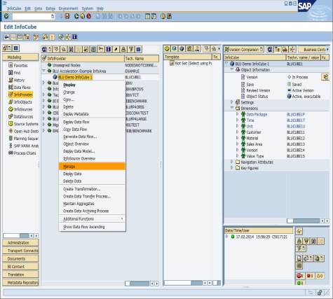
Figure 8-25 Call-up of the InfoCube administration window in the SAP BW Datawarehousing Workbench
Figure 8-26 shows the “Performance” tab page of the InfoCube administration window that has the following options:
•Delete DB Indexes (Now)
•Repair DB Indexes (Now)
•Create DB Index (Batch)
•Delete DB Index (Batch)
These options perform no work on BLU Acceleration InfoCubes.

Figure 8-26 InfoCube index and statistics management panel
As for row-organized tables, DB2 collects statistics on BLU Acceleration tables automatically. You might still want to include statistics collection into your data load process chains to make sure that InfoCube statistics are up-to-date immediately after new data was loaded.
SAP BW transaction RSRV provides an option to check and repair the indexes of an InfoCube. You can run this check also for BLU Acceleration InfoCubes. Figure 8-27 shows “Database indexes of InfoCube and its Aggregates” is run for the BLU Acceleration InfoCube BLUCUBE1.

Figure 8-27 SAP BW Transaction RSRV: InfoCube index check and repair function
The result is shown in Figure 8-28. Only the unique constraint that is defined on the E fact table and the unique constraints that are defined on the dimension tables are listed.
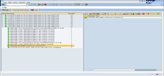
Figure 8-28 Result of index check for sample BLU Acceleration InfoCube
Figure 8-29 shows the output for the row-organized InfoCube ROWCUBE1 in comparison. For this InfoCube, many more indexes are listed.

Figure 8-29 Comparison of index check output of BLU Acceleration InfoCube with row-organized InfoCube
8.5.2 Flat InfoCubes in SAP BW 7.40
This section provides information about flat InfoCubes, which become available for DB2 as of SAP BW 7.40 Support Package 8. We show how to create flat InfoCubes and how to convert existing standard InfoCubes to flat InfoCubes. We illustrate the procedure with an example in an SAP BW 7.40 system in which the BI DataMart Benchmark InfoCubes have been installed (InfoArea BI Benchmark).
Note the following important information about flat InfoCubes:
•Flat InfoCubes are only supported with DB2 for LUW Cancun Release 10.5.0.4 and higher. The tables of flat InfoCubes are always created as column-organized tables. For optimal performance of reporting on flat InfoCubes the InfoObjects that are referenced by the InfoCubes should also be implemented with column-organized tables (see 8.5.4, “Column-Organized InfoObjects in SAP BW” on page 332).
•Both cumulative and non-cumulative InfoCubes can be created as flat InfoCubes. However, DB2 does not support the creation of real-time InfoCubes as flat InfoCubes.
•Flat InfoCubes cannot be created directly in the Data Warehousing Workbench. You must create a standard InfoCube first and then convert it to flat with report RSDU_REPART_UI.
•You can also convert existing standard InfoCubes that contain data to flat InfoCubes with report RSDU_REPART_UI.
•When you install InfoCubes from the SAP BI Content, they are created as non-flat InfoCubes. If you want these InfoCubes to be flat you need to convert them with report RSDU_REPART_UI.
•If you want to create a flat semantically partitioned InfoCube, you must first create a non-flat InfoCube and then convert the InfoCubes of which the semantically partitioned InfoCube consists to flat InfoCubes with report RSDU_REPART_UI.
•When you create a flat InfoCube and transport it to another SAP BW system, the following is created in the target system:
– If the InfoCube already exists in the target system, the target system settings are preserved, that is:
• If the InfoCube is flat in the target system it remains flat.
• If the InfoCube is non-flat in the target system it remains non-flat.
– If the InfoCube does not yet exist in the target system it is created as non-flat InfoCube and has to be converted to flat with report RSDU_REPART_UI.
Follow these steps to create a new flat InfoCube:
1. Create a new InfoCube in the Data Warehousing Workbench. New InfoCubes are always created as standard non-flat InfoCubes with two fact tables and up to 16 dimension tables.
2. Run report RSDU_REPART_UI to schedule and run a batch job that converts the standard InfoCube into a flat InfoCube.
In the following example, the creation of a flat InfoCube is shown that illustrates these steps in more detail:
1. Call transaction RSA1 to get to the Data Warehousing Workbench. In the InfoArea BI Benchmark, select Benchmark InfoCube 01 (technical name is /BIB/BENCH01), and choose Copy from the context menu (Figure 8-30).

Figure 8-30 Create a copy of InfoCube /BIB/BENCH01
2. In the Edit InfoCube window, enter FLATCUBE1 as the technical name, BLU Flat Demo InfoCube 1 as the description, and select EXAMPLE (BLU Acceleration Example InfoArea) as the InfoArea. Click the Create icon (Figure 8-31).

Figure 8-31 Create InfoCube window for InfoCube FLATCUBE1
3. The “Edit InfoCube” window in the Data Warehousing Workbench opens. Save and activate the InfoCube (Figure 8-32 on page 300). You do not need to choose between index clustering, multi-dimensional clustering (MDC) or column-organized tables in the Clustering dialog because it is not important how the InfoCube tables are created. When you convert the InfoCube to a flat InfoCube new column-organized tables are created for the InfoCube.

Figure 8-32 Edit InfoCube window for InfoCube FLATCUBE1
4. First the InfoCube is created as an enhanced star schema InfoCube with two fact and 16 dimension tables. You can check this by displaying the list of database tables that were created for the InfoCube: Choose Extras → Information (logs/status) from the menu. The “Info Selection” pop-up window is shown. Choose Dictionary/DB Status (Figure 8-33).
Figure 8-33 Info Selection window for InfoCube FLATCUBE1
5. You see the list of tables (Figure 8-34).

Figure 8-34 List of database tables of InfoCube FLATCUBE1 before conversion to a flat InfoCube
6. Double-click the F fact table /BIC/FFLATCUBE1. In the Dictionary: Display Table window, you see that the table has 8 dimension key columns and 16 key figures (Figure 8-35).
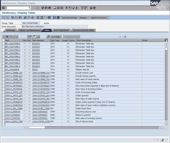
Figure 8-35 Display of F fact table of InfoCube FLATCUBE1 before conversion to a flat InfoCube
7. You have to convert the InfoCube to a flat InfoCube using report RSDU_REPART_UI: Make sure that you switch from Edit mode to Display mode in the Data Warehousing Workbench or that you close the Data Warehousing Workbench so that the InfoCube is not locked in the SAP BW system. Call transaction SE38 and run report RSDU_REPART_UI (Figure 8-36).
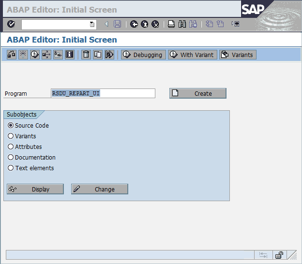
Figure 8-36 Report for converting standard InfoCubes to flat InfoCubes
8. Enter the name of the InfoCube (FLATCUBE1) in the InfoCube entry field and select Non-flat to flat conversion. For the conversion, a batch job is created that you can schedule. Choose Initialize (Figure 8-37 on page 304).
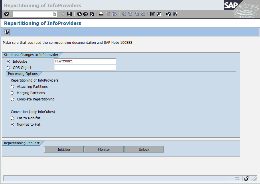
Figure 8-37 Initialize flat InfoCube conversion
9. Several pop-up windows with questions are shown. These questions are important when you convert InfoCubes that contain data to flat InfoCubes. In the current example, where the InfoCube is new and thus empty, you can answer these questions with Yes:
– Confirm that you have taken a database backup (Figure 8-38).

Figure 8-38 Inquiry about database backup
This is important when you convert existing InfoCubes with data to flat InfoCubes. During the conversion, new database tables are created, the data is copied to the new tables and the old tables are dropped. When you have a database backup, you can always go back to the state before the conversion was started.
– Confirm that you have compressed all requests that contain historical movements (Inquiry about compression of requests with historical movements). See Figure 8-39.
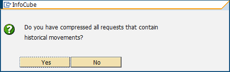
Figure 8-39 Inquiry about compression of requests with historical movements
This is important when you convert existing InfoCubes with data to flat InfoCubes. When you compress historical movements of non-flat InfoCubes, you set the “No Marker Update” flag in the compression window. For flat InfoCubes, this is handled differently: you define directly in the Data Transfer Process (DTP) whether you load requests that contain historical movements. However, this only has an effect for requests that are newly loaded after the conversion of the InfoCube to a flat InfoCube. For requests that already reside in the F fact table, it is no longer possible to detect and correctly compress requests that contain historical movements after the InfoCube conversion to a flat InfoCube.
|
Note: When you convert existing InfoCubes with data, the report checks whether any uncompressed requests with package dimension ID 1 or 2 exist. If this is the case you must compress these requests before the conversion. The package dimension IDs 1 and 2 are reserved for marker records of non-cumulative InfoCubes and for historical movement data in flat InfoCubes.
|
10. The information message shown in Figure 8-40 is displayed.
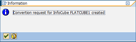
Figure 8-40 Message about flat InfoCube conversion job creation
When you confirm the message, the “Start Time” window in Figure 8-41 is shown.
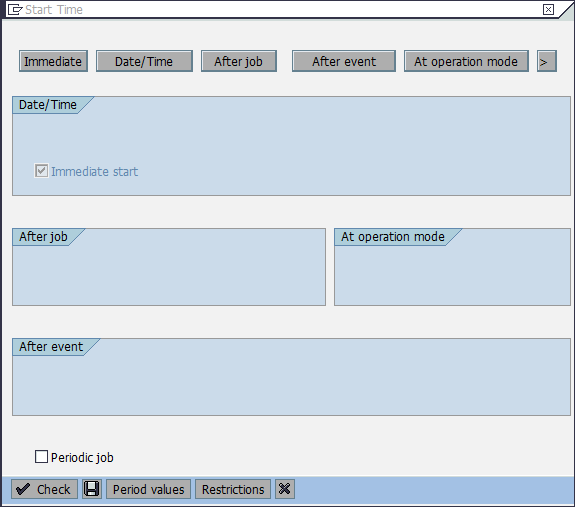
Figure 8-41 Schedule flat InfoCube conversion job
Choose Immediate as start time for the conversion batch job and choose Enter. The following information message is shown (Figure 8-42).

Figure 8-42 Message about start of flat InfoCube conversion job
11. On the window of report RSDU_REPART_UI, choose Monitor to track the progress of the conversion until it is finished successfully (Figure 8-43).

Figure 8-43 Successful conversion of InfoCube FLATCUBE1 to a flat InfoCube
12. Go back to the Data Warehousing Workbench and display the InfoCube FLATCUBE1 (Figure 8-44).

Figure 8-44 Edit InfoCube window for flat InfoCube FLATCUBE1
13. Choose Extras → Information (logs/status) from the menu. From the Info Selection pop-up window, select Dictionary/DB status. Now the list of InfoCube tables only contains two tables: the F fact table and the package dimension table (Figure 8-45).

Figure 8-45 Overview of database tables of flat InfoCube FLATCUBE1
14. Double-click the F fact table /BIC/FFLATCUBE1 to get to the SAP Data Dictionary.
The table fields contain the package dimension key column, 14 columns for the SIDs of all the characteristics, and the 16 key figure columns (Figure 8-46).
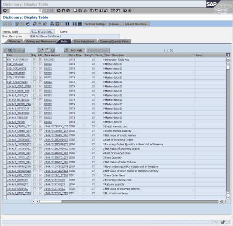
Figure 8-46 Display table /BIC/FFLATCUBE1
15. Choose Utilities → Database Object → Database Utility from the menu and select Storage Parameters. In the storage parameters window, you see that the table is column-organized (Figure 8-47).

Figure 8-47 Storage parameters of fact table of flat InfoCube FLATCUBE1
16. Repeat steps 14 and 15 for the package dimension table. You see that the package dimension table is also column-organized.
Table layout of flat InfoCubes
You can use the DB2 db2look tool to extract the DDL for the fact table:
db2look -d D01 -a -e -t "/BIC/FFLATCUBE1"
Example 8-11 shows the DDL of the table.
Example 8-11 DDL describing the fact table of a flat InfoCube
CREATE TABLE "SAPPB3 "."/BIC/FFLATCUBE1" (
"KEY_FLATCUBE1P" INTEGER NOT NULL WITH DEFAULT 0 ,
"/B49/S_BASE_UOM" INTEGER NOT NULL WITH DEFAULT 0 ,
"/B49/S_DISTR_CHA" INTEGER NOT NULL WITH DEFAULT 0 ,
"/B49/S_DIVISION" INTEGER NOT NULL WITH DEFAULT 0 ,
"/B49/S_MATERIAL" INTEGER NOT NULL WITH DEFAULT 0 ,
"/B49/S_SALESORG" INTEGER NOT NULL WITH DEFAULT 0 ,
"/B49/S_SOLD_TO" INTEGER NOT NULL WITH DEFAULT 0 ,
"/B49/S_STAT_CURR" INTEGER NOT NULL WITH DEFAULT 0 ,
"/B49/S_VERSION" INTEGER NOT NULL WITH DEFAULT 0 ,
"/B49/S_VTYPE" INTEGER NOT NULL WITH DEFAULT 0 ,
"SID_0CALDAY" INTEGER NOT NULL WITH DEFAULT 0 ,
"SID_0CALMONTH" INTEGER NOT NULL WITH DEFAULT 0 ,
"SID_0CALWEEK" INTEGER NOT NULL WITH DEFAULT 0 ,
"SID_0FISCPER" INTEGER NOT NULL WITH DEFAULT 0 ,
"SID_0FISCVARNT" INTEGER NOT NULL WITH DEFAULT 0 ,
"/B49/S_CRMEM_CST" DECIMAL(17,2) NOT NULL WITH DEFAULT 0 ,
"/B49/S_CRMEM_QTY" DECIMAL(17,3) NOT NULL WITH DEFAULT 0 ,
"/B49/S_CRMEM_VAL" DECIMAL(17,2) NOT NULL WITH DEFAULT 0 ,
"/B49/S_INCORDCST" DECIMAL(17,2) NOT NULL WITH DEFAULT 0 ,
"/B49/S_INCORDQTY" DECIMAL(17,3) NOT NULL WITH DEFAULT 0 ,
"/B49/S_INCORDVAL" DECIMAL(17,2) NOT NULL WITH DEFAULT 0 ,
"/B49/S_INVCD_CST" DECIMAL(17,2) NOT NULL WITH DEFAULT 0 ,
"/B49/S_INVCD_QTY" DECIMAL(17,3) NOT NULL WITH DEFAULT 0 ,
"/B49/S_INVCD_VAL" DECIMAL(17,2) NOT NULL WITH DEFAULT 0 ,
"/B49/S_OPORDQTYB" DECIMAL(17,3) NOT NULL WITH DEFAULT 0 ,
"/B49/S_OPORDVALS" DECIMAL(17,2) NOT NULL WITH DEFAULT 0 ,
"/B49/S_ORD_ITEMS" DECIMAL(17,3) NOT NULL WITH DEFAULT 0 ,
"/B49/S_RTNSCST" DECIMAL(17,2) NOT NULL WITH DEFAULT 0 ,
"/B49/S_RTNSQTY" DECIMAL(17,3) NOT NULL WITH DEFAULT 0 ,
"/B49/S_RTNSVAL" DECIMAL(17,2) NOT NULL WITH DEFAULT 0 ,
"/B49/S_RTNS_ITEM" DECIMAL(17,3) NOT NULL WITH DEFAULT 0 )
DISTRIBUTE BY HASH("/B49/S_SOLD_TO",
"/B49/S_MATERIAL",
"/B49/S_DISTR_CHA",
"/B49/S_VERSION",
"/B49/S_VTYPE",
"SID_0CALDAY",
"/B49/S_BASE_UOM")
IN "PB3#FACTD" INDEX IN "PB3#FACTI"
ORGANIZE BY COLUMN;
Use the following command to get the DDL of the package dimension table.
db2look -d D01 -a -e -t "/BIC/FFLATCUBE1"
Example 8-12 shows the result.
Example 8-12 DDL describing the package dimension table of a flat InfoCube
CREATE TABLE "SAPPB3 "."/BIC/DFLATCUBE1P" (
"DIMID" INTEGER NOT NULL WITH DEFAULT 0 ,
"SID_0CHNGID" INTEGER NOT NULL WITH DEFAULT 0 ,
"SID_0RECORDTP" INTEGER NOT NULL WITH DEFAULT 0 ,
"SID_0REQUID" INTEGER NOT NULL WITH DEFAULT 0 )
IN "PB3#DIMD" INDEX IN "PB3#DIMI"
ORGANIZE BY COLUMN;
-- DDL Statements for Primary Key on Table "SAPPB3 "."/BIC/DFLATCUBE1P"
ALTER TABLE "SAPPB3 "."/BIC/DFLATCUBE1P"
ADD CONSTRAINT "/BIC/DFLATCUBE1P~0" PRIMARY KEY
("DIMID");
-- DDL Statements for Unique Constraints on Table "SAPPB3 "."/BIC/DFLATCUBE1P"
ALTER TABLE "SAPPB3 "."/BIC/DFLATCUBE1P"
ADD CONSTRAINT "/BIC/DFLATCUBE1P99" UNIQUE
("SID_0CHNGID",
"SID_0RECORDTP",
"SID0REQUID");
Flat InfoCube index, statistics, and space management
The fact table of flat InfoCubes has no primary key or unique constraint and no secondary indexes. Therefore overhead for index management does not occur.
The “Performance” tab of the SAP BW administration window for flat InfoCubes (Figure 8-48) does not contain any options for aggregates because aggregates cannot be defined on flat InfoCubes.
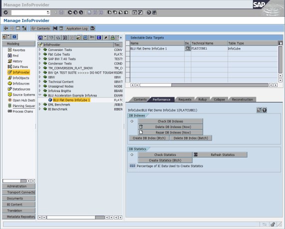
Figure 8-48 Manage flat InfoCube FLATCUBE1 - Performance tab
The “DB indexes” options perform no work on flat InfoCubes.
SAP BW transaction RSRV provides an option to check and repair the indexes of an InfoCube. You can run this check also for flat InfoCubes. Figure 8-49 shows “Database indexes of InfoCube and its Aggregates” is run for the BLU Acceleration InfoCube FLATCUBE1.

Figure 8-49 Check database indexes of flat InfoCube FLATCUBE1
The result is shown in Figure 8-50. Only the unique constraint that is defined on the package dimension table is listed.
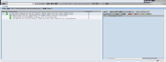
Figure 8-50 Result of database index check for flat InfoCube FLATCUBE1
8.5.3 Column-Organized DataStore Objects (DSOs) in SAP BW
In this section, we show how to create standard and write-optimized DSOs such that the active table is created as column-organized table. We illustrate the procedure with an example in an SAP BW 7.40 system in which the BI DataMart Benchmark InfoCubes have been installed (InfoArea BI Benchmark). The example works in exactly the same way in the other SAP BW releases in which BLU Acceleration for DSOs is supported.
The creation of DSOs with a column-organized active table is supported as of DB2 for LUW Cancun Release 10.5.0.4 and in SAP BW as of SAP BW 7.0. For detailed information about the required SAP Support Packages and SAP Notes see 8.2, “Prerequisites and restrictions for using BLU Acceleration in SAP BW”.
Creating DSOs with a column-organized active table can have the following advantages:
•Compression of the active table can be improved because column-organized tables usually compress better than row-organized tables.
•Reporting queries on DataStore objects run faster. You can run more queries directly on DataStore objects. This can eliminate the need for creating InfoCubes which saves both storage space and ETL processing time for propagating data from DataStore objects into InfoCubes. For optimal performance of reporting on DSOs, the InfoObjects that occur in the DSOs should also be implemented with column-organized tables (see 8.5.4, “Column-Organized InfoObjects in SAP BW” on page 332).
Both standard and write-optimized DSOs can be created with column-organized active tables. The activation queue and change log tables of standard DSOs are still created row-organized.
You can convert existing DSOs with row-organized active tables to column-organized with DB6CONV (see 8.6.1, “Conversion of SAP BW objects to column-organized tables with DB2 Cancun Release 10.5.0.4 and DB6CONV V6” on page 351).
Creating column-organized standard DSO
We create a new standard DSO from a DataSource as follows:
1. Call transaction RSA1 and select DataSources from the Modelling window. Open the “Benchmark” folder, select DataSource BENCH_DTP_CUBE1 and call up Generate Data Flow from the context menu (Figure 8-51).
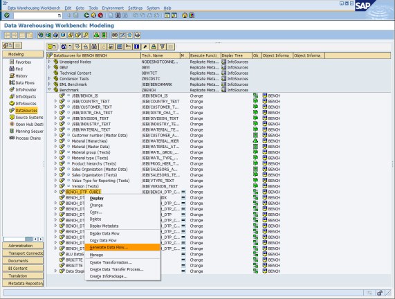
Figure 8-51 Generate new DSO from DataSource with Data Flow Generation
2. In the Data Flow Generation Wizard, select DataStore Object as InfoProvider type, Standard as Subtype, enter BLUDSO1 as InfoProvider name, BLU DEMO DSO 1 as description, and EXAMPLE as InfoArea, and choose Continue (Figure 8-52).

Figure 8-52 Define new target DSO of Data Flow

Figure 8-53 Field assignment window of Data Flow Generation wizard
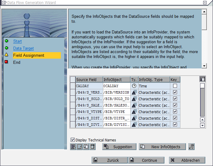
Figure 8-54 Define InfoObects of new DSO in Data Flow Generation wizard

Figure 8-55 Final window of Data Flow Generation wizard
6. In transaction RSA1, select InfoProvider from the Modelling window. In the “EXAMPLE InfoArea”, you find the newly created standard DSO. Open the DSO in Edit mode (Figure 8-56).

Figure 8-56 Edit standard DSO
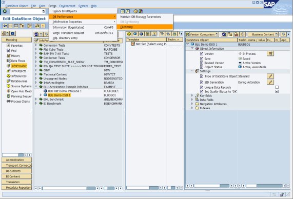
Figure 8-57 Define clustering for standard DSO

Figure 8-58 Clustering window of standard DSO
9. Save and activate the DSO. Then select Extras → Information (logs/status) from the menu (Figure 8-59 on page 324).

Figure 8-59 Show database tables of standard DSO
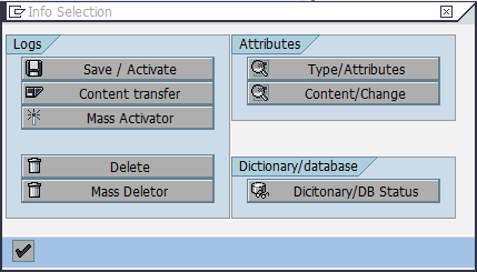
Figure 8-60 Info Selection window for standard DSO
11. In the Status information window, double-click the name of the “Active Table” /BIC/ABLUDSO100 (Figure 8-61) to get to the SAP Data Dictionary.
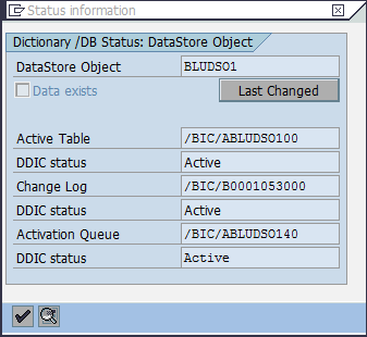
Figure 8-61 Database tables of standard DSO
In the SAP Data Dictionary, look up the storage parameters of the table as described in step 2 on page 262. The storage parameters show that the table is column-organized (Figure 8-62).
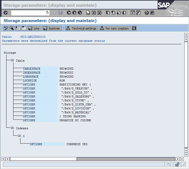
Figure 8-62 Storage parameters of BLU standard DSO active table
Creating column-organized write-optimized DSO
We create a write-optimized DSO by copying the standard DSO BLUDSO1 that we created in the previous chapter as follows:
1. In transaction RSA1, select standard DSO BLUDSO1 and choose Copy... from the context menu (Figure 8-63 on page 327).
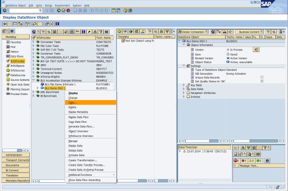
Figure 8-63 Copy DSO
2. In the Create DataStore Object window enter BLUWDSO1 as technical name and “BLU Demo write-optimized DSO 1” as description and click the Create icon (Figure 8-64).

Figure 8-64 Create DataStore Object window
3. In the “Edit DataStore Object” window change the type of the DSO in the “Settings” folder from “Standard” to “Write Optimized” (Figure 8-65).

Figure 8-65 Change DSO type to write-optimized from standard

Figure 8-66 Define clustering for write-optimized DSOs

Figure 8-67 Clustering window for write-optimized DSOs
6. Save and activate the write-optimized DSO and select Extras → Information (logs/status) from the menu (Figure 8-68 on page 330).
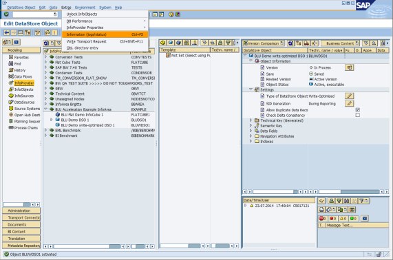
Figure 8-68 Prepare to display database tables of write-optimized DSO
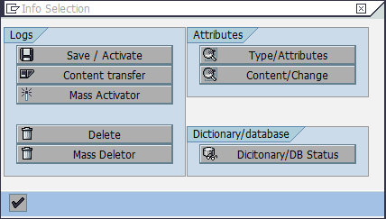
Figure 8-69 Info Selection window for write-optimized DSO
8. In the “Status information” window double-click the name of the “Active Table” to get to the SAP Data Dictionary (Figure 8-70 on page 331).

Figure 8-70 Overview of database tables of write-optimized DSO
9. Look up the storage parameters for the table as described in step 2 on page 262. The storage parameters show that the table is column-organized (Figure 8-71 on page 331).
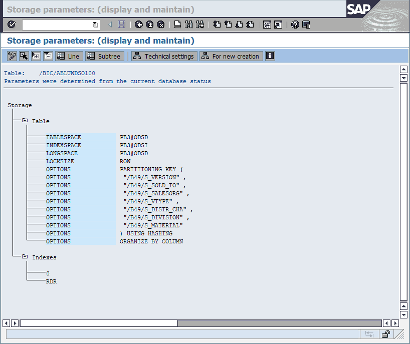
Figure 8-71 Storage parameters of column-organized write-optimized DSO
8.5.4 Column-Organized InfoObjects in SAP BW
In this section, we show how to create InfoObjects, such as the InfoObject tables that occur in SAP BW reporting queries, as column-organized tables.
We illustrate the procedure with an example in an SAP BW 7.40 system in which the BI DataMart Benchmark InfoCubes have been installed (InfoArea BI Benchmark). The example works in exactly the same way in the other SAP BW releases in which BLU Acceleration is supported.
The creation of InfoObjects with column-organized tables is supported as of DB2 for LUW Cancun Release 10.5.0.4 and in SAP BW as of SAP BW 7.0. For detailed information about the required SAP Support Packages, see 8.2, “Prerequisites and restrictions for using BLU Acceleration in SAP BW”.
Creating InfoObjects with column-organized tables can improve query performance when the InfoObject tables are joined with column-organized InfoCube or DSO tables. You can convert existing InfoObjects that use row-organized tables to column-organized tables with DB6CONV (see 8.6.1, “Conversion of SAP BW objects to column-organized tables with DB2 Cancun Release 10.5.0.4 and DB6CONV V6” on page 351).
From the tables that are created for an InfoObject, only the SID table (S table) and the time-dependent and time-independent attribute SID tables (X and Y tables) are created as column-organized tables. These are the tables that frequently occur in SAP BW reporting queries. The text table, the time-dependent and time independent attribute tables, and the hierarchy tables remain row-organized.
By default, SAP BW InfoObjects are created with row-organized tables only. SAP BW provides the RSADMIN configuration parameter, DB6_IOBJ_USE_CDE, to create SID and attribute SID tables as column-organized tables. You set this parameter as follows:
1. Call transaction SE38 and run the SAP_RSADMIN_MAINTAIN report.
2. In the “OBJECT” field, enter DB6_IOBJ_USE_CDE. In the “VALUE” field, enter YES, and then click the Execute icon (Figure 8-72).
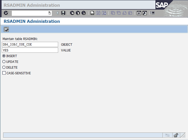
Figure 8-72 Report SAP_RSADMIN_MAINTAIN: Set option to create SAP BW InfoObject tables column-organized
The information shown in Figure 8-73 is displayed.
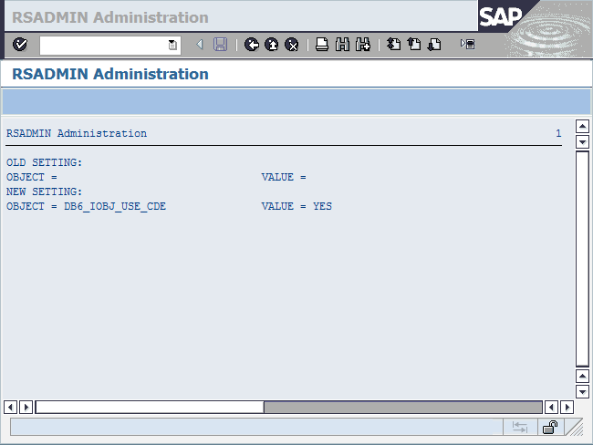
Figure 8-73 Report SAP_RSADMIN_MAINTAIN: Result of setting the option to create SAP BW InfoObject tables column-organized
Now create a copy of the /BIB/MATERIAL InfoObject as follows:
1. Call transaction RSD1.

Figure 8-74 Edit InfoObjects: Start window
3. Click the Copy icon. In the pop-up window (Figure 8-75) enter “BLU Material InfoObject” as Long Description and /BIB/MATERIAL in the “Template” entry field.
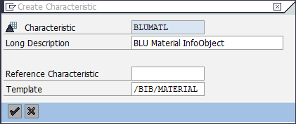
Figure 8-75 Create Characteristic window
4. The “Create Characteristic BLUMATL: Detail” window is displayed (see Figure 8-76). Save and activate the InfoObject.
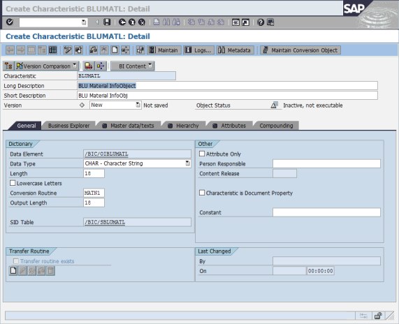
Figure 8-76 Create BLU Material InfoObject Detail window

Figure 8-77 BLU Material InfoObject Edit window
Information about the tables created for the InfoObject is displayed (Figure 8-78).

Figure 8-78 Overview of tables of BLU Material InfoObject
6. Double-click the SID table name /BIC/SBLUMATL. In the SAP Data Dictionary look up the storage parameters with the Database Utility. In the storage parameters you see that the table is column-organized (Figure 8-79).

Figure 8-79 Storage parameters of BLU Material SID table
7. Repeat step 6 on page 339 for the tables /BIC/XBLUMATL and /BIC/PBLUMATL. You see that table /BIC/XBLUMATL is also column-organized (Figure 8-81) and that table /BIC/PBLUMATL is row-organized (Figure 8-80). All other tables of the InfoObject are also row-organized.
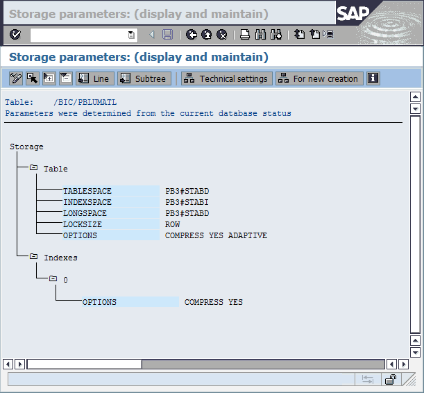
Figure 8-80 Storage parameters of BLU Material display attribute table

Figure 8-81 Storage parameters of BLU Material attribute SID table
8.5.5 Column-organized PSA tables in SAP BW
In this section, we show how to create PSA tables as column-organized tables.
We illustrate the procedure with an example in an SAP BW 7.40 system in which the EML Benchmark InfoCubes and DataStore objects have been installed (InfoArea EML Benchmark). The example works in exactly the same way in the other SAP BW releases in which BLU Acceleration is supported.
The creation of column-organized PSA tables is supported as of DB2 for LUW Cancun Release 10.5.0.4 and in SAP BW as of SAP BW 7.0. For detailed information about the required SAP Support Packages, see 8.2, “Prerequisites and restrictions for using BLU Acceleration in SAP BW”.
Creating PSA tables as column-organized tables might improve compression because column-organized tables usually compress better than row-organized tables. You can convert existing row-organized PSA tables to column-organized tables with DB6CONV (see 8.6.1, “Conversion of SAP BW objects to column-organized tables with DB2 Cancun Release 10.5.0.4 and DB6CONV V6” on page 351).
By default, PSA tables are created row-organized. SAP BW provides the RSADMIN configuration parameter DB6_PSA_USE_CDE to create PSA tables as column-organized tables. You set this parameter as follows:
1. Call transaction SE38 and run the SAP_RSADMIN_MAINTAIN report.
2. In the “OBJECT” field, enter DB6_PSA_USE_CDE. In the “VALUE” field, enter YES, and then click the Execute icon (Figure 8-82).

Figure 8-82 Report SAP_RSADMIN_MAINTAIN: Set option to create SAP BW PSA tables column-organized
The information shown in Figure 8-83 is displayed.
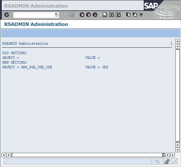
Figure 8-83 Report SAP_RSADMIN_MAINTAIN: Result of setting the option to create SAP BW PSA tables column-organized
Now you can create a new DataSource as follows:
1. Call transaction RSA1 and select DataSources in the Modelling window. Open the Benchmark folder, select DataSource BENCH_DTP_CUBE1, and choose Copy from the context menu (Figure 8-84).

Figure 8-84 Copy an existing SAP BW DataSource
2. In the Target frame enter BLUDS1 as “DataSource” name and BENCH as “Source system” and press Enter (Figure 8-85).

Figure 8-85 Copy DataSource window
Enter “BLU DataSource 1” as short, medium, and long description and save and activate the DataSource (Figure 8-86).

Figure 8-86 Properties of an SAP BW DataSource
3. Select Goto → Technical Attributes from the menu. The technical attributes window is shown (Figure 8-87).

Figure 8-87 Technical Attributes of an SAP BW DataSource
4. Double-click the PSA table to get to the SAP Data Dictionary and look up the storage parameters of the table as described in step 2 on page 262. The storage parameters show that the table is column-organized (Figure 8-88).
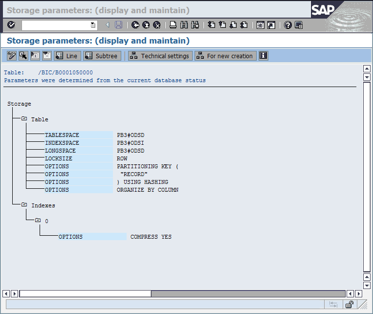
Figure 8-88 Storage parameters of BLU PSA table
8.5.6 Column-organized temporary tables in SAP BW
When running SAP BW queries, intermediate results are often calculated and stored in database tables. These tables are called “SAP BW temporary tables”. The following temporary table types for InfoCube queries are the most important:
•Temporary hierarchy (02) tables (naming convention is /BI0/02<number>)
These tables store results from the evaluation of master data hierarchies. The data in these tables can be used by multiple SAP BW queries and is therefore preserved for a longer period of time.
•EQSID (06) tables (naming convention is /BI0/06<number>)
These tables are used to store SIDs of master data. They are used to avoid large IN-lists in the WHERE condition of SQL queries.
•Temporary pre-materialization (0P) tables (naming convention is /BI0/0P<number>):
These tables are used to store the results of joins of master data and dimension tables. They are used for SQL queries that join a large number of tables. These queries are split in a way that the result of the join of each dimension table with master data tables is calculated separately and stored in a 0P table. A final SQL query then joins the fact tables with the 0P tables.
Creating SAP BW temporary tables as column-organized tables can improve the performance of queries on BLU Acceleration InfoCubes. By default, SAP BW temporary tables are created as row-organized tables. SAP BW provides the RSADMIN configuration parameter, DB6_TMP_USE_CDE, to create SAP BW temporary tables as column-organized tables. You set this parameter as follows:
1. Call transaction SE38 and run the SAP_RSADMIN_MAINTAIN report.
2. In the “OBJECT” field, enter DB6_TMP_USE_CDE. In the VALUE field, enter YES, and then click the Execute icon (Figure 8-89).
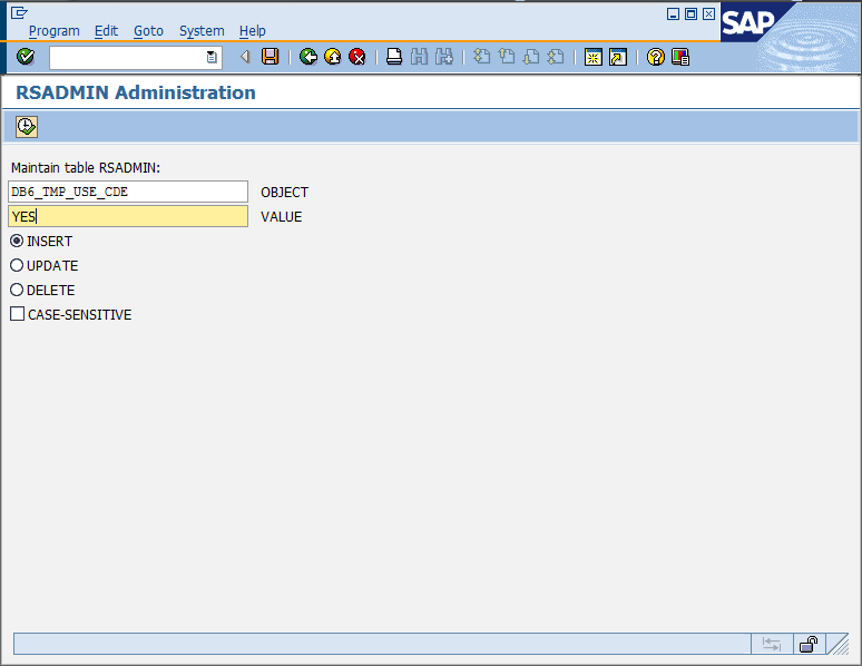
Figure 8-89 Report SAP_RSADMIN_MAINTAIN: Set option to create SAP BW temporary tables column-organized
The information shown in Figure 8-90 is displayed.

Figure 8-90 Report SAP_RSADMIN_MAINTAIN: Result of setting the option to create SAP BW temporary tables column-organized
Consider this information about column-organized temporary tables in SAP BW:
•SAP BW temporary tables are visible in the ABAP Dictionary. You can check whether a temporary table is a column-organized table by inspecting the storage parameters of the table. See 8.3, “BLU Acceleration support in the ABAP Dictionary” on page 261.
•Changes to the RSADMIN parameter, DB6_TMP_USE_CDE, have an effect only when new SAP BW temporary tables are created. There is no effect on existing tables. Temporary hierarchy tables and EQSID tables are managed in a pool and reused. Therefore, a large number of row-organized temporary tables might exist already when you set the RSADMIN parameter. When you start working with BLU Acceleration InfoCubes, drop existing temporary tables and set the RSADMIN parameter so that new temporary tables are created as column-organized tables. You can drop temporary tables with the SAP_DROP_TMPTABLES report. Before you drop temporary tables, make sure that you read SAP Note 1139396.
When you have a mixture of row-organized and column-organized InfoCubes in your system and generate SAP BW temporary tables as column-organized tables, these column-organized temporary tables might be used in queries on row-organized InfoCubes. This might cause a small performance penalty. However, this is outweighed by the performance benefit for queries on column-organized InfoCubes.
8.6 Conversion of SAP BW objects to column-organized tables
You can convert existing InfoCubes, DSOs, InfoObjects, and PSA tables from row-organized to column-organized tables with the conversion report DB6CONV. The conversion of standard column-organized InfoCubes to flat ones has to be done separately as described in 8.5.2, “Flat InfoCubes in SAP BW 7.40” on page 297.
When you have installed DB2 10.5 FP3SAP BLU Acceleration is only supported for InfoCubes. In this case you must use the report SAP_CDE_CONVERSION_DB6 to convert existing InfoCubes to column-organized tables. SAP_CDE_CONVERSION_DB6 creates a table conversion job that you can schedule and run with DB6CONV. This is described in detail in 8.6.2, “Conversion of InfoCubes to column-organized tables before DB2 Cancun Release 10.5.0.4”.
When you have installed DB2 Cancun Release 10.5.0.4 and DB6CONV V6 you can generate conversion jobs for InfoCubes, DSOs, InfoObjects, and PSA tables directly with the DB6CONV tool. You do not need the report SAP_CDE_CONVERSION_DB6.
8.6.1 Conversion of SAP BW objects to column-organized tables with DB2 Cancun Release 10.5.0.4 and DB6CONV V6
DB6CONV V6 provides a new tab page for the conversion of SAP BW object tables from row-organized to column-organized and vice versa. You can convert single, selected, or all InfoCubes, DSOs, InfoObjects, and PSA tables. DB6CONV collects the tables of the selected BW objects that need to be converted and puts them into a DB6CONV job.
You can schedule and run the job like any other DB6CONV table or table space conversion jobs:
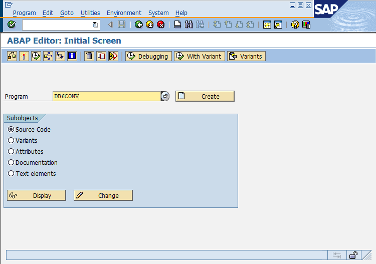
Figure 8-91 Invocation of report DB6CONV
The DB6CONV conversion window is shown (see Figure 8-92).
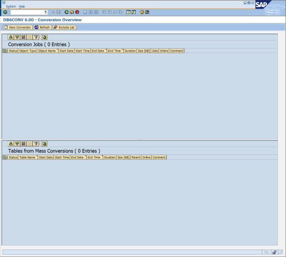
Figure 8-92 DB6CONV Tool - Conversion jobs overview
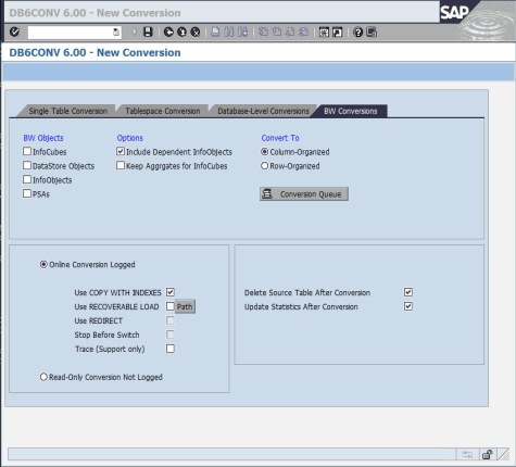
Figure 8-93 DB6CONV Tool - BW Conversions
3. You can convert InfoCubes, DSOs, InfoObjects, and PSA tables from row-organized to column-organized tables and vice versa. The following options are available:
– Include Dependent InfoObjects: If you use this option, the InfoObjects that are referenced in the InfoCubes and DSOs to be converted are included in the conversion job. Inclusion of InfoObjects is the default because reporting performance usually improves if the InfoObject tables that are referenced in the queries have the same layout as the InfoCube or DSO tables. If you do not want to convert InfoObjects, you must deselect this option.
– Keep Aggregates for InfoCubes: For conversions from row-organized to column-organized tables, the default is not to keep the InfoCube aggregates. In most cases the aggregates are no longer needed because the InfoCube queries run fast enough on the InfoCube itself. Therefore the aggregates are deactivated when the InfoCube tables have been converted to column-organized tables. The definitions of the aggregates are kept in the SAP BW metadata so that selected aggregates can be re-activated and filled if needed.
For conversions of column-organized to row-organized tables, the default is to keep the InfoCube aggregates. In such a conversion, the aggregate tables are also converted to row-organized tables.
The following conversion methods are offered:
– Online Conversion Logged: With this conversion method, DB6CONV creates the target table and then calls the AMDIN_MOVE_TABLE stored procedure to create the indexes (optional) and copy the data. The following options for ADMIN_MOVE_TABLE are available:
• Use COPY WITH INDEXES: This option is the default and should not be changed. ADMIN_MOVE_TABLE takes care of the conversion of unique and primary key indexes on row-organized tables to BLU constraints and vice versa. Non-unique indexes on the row-organized tables are not created on target column-organized tables.
• Use RECOVERABLE LOAD: When this option is selected, ADMIN_MOVE_TABLE uses LOAD WITH COPY YES to copy the data. Choose Path to specify a location for the LOAD COPY files.
• Trace (Support Only): With this option, an ADMIN_MOVE_TABLE trace in the db2dump directory is created. This can be useful to identify issues in support situations, but it generates a significant performance overhead as well.
– Read-Only Conversion Not Logged: With this conversion method, DB6CONV creates the target table and its indexes or constraints and uses the non-recoverable DB2 LOAD to copy the data from the source to the target tables.
In the following example, you convert two row-organized InfoCubes to column-organized without InfoObjects:
1. Select InfoCubes, de-select Include Dependent InfoObjects, and choose Conversion Queue (Figure 8-94).

Figure 8-94 DB6CONV - Conversion of InfoCube tables to column-organized tables
2. A pop-up window with all basic row-organized InfoCubes in the system is shown (Figure 8-95). In the header, the number of InfoCubes and the number of database tables and their overall size is displayed.
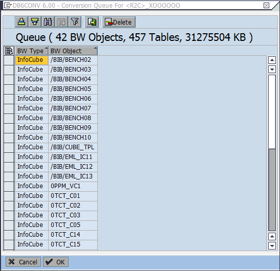
Figure 8-95 DB6CONV - Conversion candidate InfoCubes
3. If you do not want to convert all InfoCubes in the list, you must select the InfoCubes that should not be converted and delete them from the list. In this example, you want to convert only the InfoCubes ROWCUBE1 and ROWCUBE2.
4. Click the icon in the top left corner of the list to select all list elements, then search for ROWCUBE1 and ROWCUBE2 (binoculars icon) and de-select these two InfoCubes only (Figure 8-96).

Figure 8-96 DB6CONV - Selection of BW Objects to be excluded
5. Then choose Delete to delete all InfoCubes except ROWCUBE1 and ROWCUBE2 from the list (Figure 8-97).
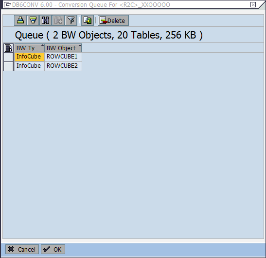
Figure 8-97 DB6CONV - Selected conversion candidates
6. When you double-click one of the two InfoCubes, the list of its database tables is displayed in a separate pop-up window (Figure 8-98).

Figure 8-98 DB6CONV - List of tables of a sample InfoCube to be converted
7. Choose OK two times to close the pop-up windows and save the conversion queue in the BW Conversions window (floppy disc icon in Figure 8-94 on page 355). The pop-up window in Figure 8-99 is shown.

Figure 8-99 DB6CONV - Information about newly created conversion job
8. When you confirm the information message, the conversion overview window is shown with the newly created conversion job with status PLANNED (see Figure 8-100).
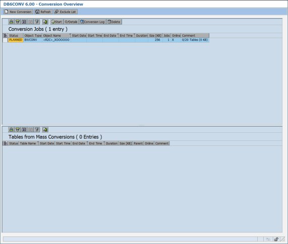
Figure 8-100 DB6CONV - Conversion jobs overview window
The object type (BWCONV) of the job indicates that this is a conversion of BW objects. The job name reflects the conversion direction (R2C = row-organized to column-organized) and the conversion options that were selected.
9. Select the job and choose Start to schedule it. The Start Conversion window is shown (Figure 8-101).

Figure 8-101 DB6CONV - Schedule a conversion job
10. We can choose the job start time and the number of parallel processes with which it is executed. Improvements in DB6CONV V6 allow to choose a much higher degree of parallelism than in previous DB6CONV versions.
During the conversion, the job status changes to RUNNING and the tables that have already been processed and that are currently being processed are listed on the Tables from Mass Conversions area in the Conversion Overview window (Figure 8-102).
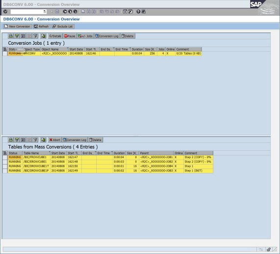
Figure 8-102 DB6CONV - Running conversion job
11. Wait until the job is finished (Figure 8-103).

Figure 8-103 DB6CONV - Completed conversion job
12. DB6CONV writes a conversion log for the complete conversion job and for each table separately. You can examine the log by double-clicking the conversion job or table or by selecting the job or table and choosing Conversion Log in the Conversion Overview window.
Figure 8-104 and Figure 8-105 show an excerpt from the conversion logs of the conversion job and of dimension table /BIC/DROWCUBE25. The log for each table log contains the conversion options that were selected in the BW Conversions tab, the CREATE TABLE statement for the target table, an overview of the indexes and constraints that are defined on the target table, and information about the ADMIN_MOVE_TABLE steps that were executed. The log of the conversion job contains information about the InfoCubes and tables that were deleted from the original conversion queue, about the parallel child jobs that executed the conversion and of required post processing steps that were executed.

Figure 8-104 DB6CONV - Sample conversion log file
13. When a conversion aborts, take the following actions:
a. For each table that failed during the conversion, examine the conversion log to identify the root cause of the failure. If you cannot solve the issue, open an incident at SAP.
b. Reset the conversion of each table that failed in the Table from Mass Conversions area in the Conversion Overview window.
c. Reset the conversion of the whole job in the Conversion Jobs area.

Figure 8-105 DB6CONV - Sample table conversion log file
8.6.2 Conversion of InfoCubes to column-organized tables before DB2 Cancun Release 10.5.0.4
SAP BW provides the SAP_CDE_CONVERSION_DB6 report for converting existing InfoCubes from row-organized to column-organized tables and vice versa if you have DB2 10.5 FP3aSAP installed. You can convert a single InfoCube or all InfoCubes in the BW system. Only the fact and dimension tables are converted. The InfoObjects that are referenced in the InfoCubes remain row-organized. The report collects the database tables for the selected InfoCube or for all InfoCubes and creates a job for the SAP DB2-specific table conversion report DB6CONV. The conversion job can be scheduled and monitored in the DB6CONV report.
To use SAP_CDE_CONVERSION_DB6, install SAP Note 1964464. This SAP Note fixes issues with respect of the handling of InfoCube aggregates.
You need at least DB6CONV V5.30 for column-organized tables to be supported. The DB6CONV report and documentation are in SAP Note 1513862. SAP recommends that you always use the latest available DB6CONV version.
It is important that you use the SAP_CDE_CONVERSION_DB6 report for the conversion to BLU Acceleration and not native DB2 tools such as db2convert or the ADMIN_MOVE_TABLE stored procedure directly. The report ensures that all InfoCube tables are converted and it ensures that the constraints on the converted tables are created as required by SAP BW.
In the following example, we use the SAP_CDE_CONVERSION_DB6 report and the DB6CONV report to convert InfoCube ROWCUBE1 to column-organized tables:
 .
.Figure 8-106 Invocation of report SAP_CDE_CONVERSION_DB6
2. You can enter the name of an InfoCube in the InfoCube field, get a list for selection of InfoCubes in the system with F4 (help), or select All InfoCubes to convert all InfoCubes in the BW system. Enter ROWCUBE1 in the InfoCube field and click Get Dependent Tables (Figure 8-107).
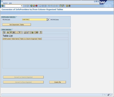
Figure 8-107 Report SAP_CDE_CONVERSION_DB6: Conversion of an InfoCube
3. The InfoCube tables are listed in the Table Selection area (Figure 8-108). The list indicates whether each table is or is not column-organized.
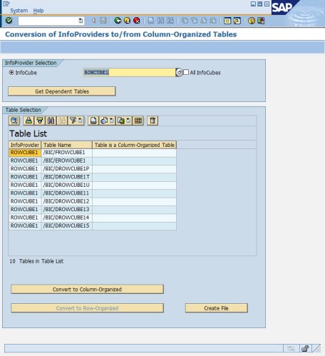
Figure 8-108 Report SAP_CDE_CONVERSION_DB6 -List of InfoCube tables to be converted
4. In this example, all tables are row-organized. You can save the table list in a file by clicking Create File, and you can create a DB6CONV conversion job by choosing Convert to Column-Organized.
When you click Convert to Column-Organized, the message in Figure 8-109 is displayed.
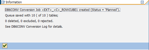
Figure 8-109 Report SAP_CDE_CONVERSION_DB6: Information about DB6CONV job
5. A DB6CONV job, <EXT>_<C>_ROWCUBE1, with 10 tables to be converted was created. The <C> in the job name indicates that this is a conversion job to column-organized tables. You schedule, run, and monitor the job using the DB6CONV report.
6. If you choose to convert all InfoCubes, all InfoCube tables are determined. Because a mixture between column-organized and row-organized InfoCubes might exist in your system, both options (Convert to Column-Organized and Convert to Row-Organized) are offered. Depending on which option you choose, a job for either the column-organized or the row-organized tables is created.
You can convert only basic InfoCubes. If the InfoCube that you want to convert has aggregates, the following options are available:
– The InfoCube is a row-organized InfoCube that you want to convert to column-organized.
In this case, you are asked whether you want to keep the aggregates or deactivate them. If you use BLU Acceleration, you do not need aggregates any more in many cases. Therefore, you might choose to deactivate the aggregates. In this case, the aggregate definitions are preserved but the aggregate database tables are dropped.
If you determine later that some of the deactivated aggregates would still be useful, you can reactivate these aggregates in the Maintenance for Aggregates window of the Data Warehousing Workbench. However, you must refill them with the data from the InfoCube. If you want to keep the aggregates when you convert an InfoCube to BLU Acceleration, the aggregate tables are included into the conversion job in such a way that they are also converted to BLU Acceleration.
– The InfoCube is a column-organized InfoCube that you want to convert back to row-organized.
In this case, the aggregate tables are automatically added to the conversion job in a way that the aggregate tables are also converted back to row-organized.
Running and monitoring InfoCube conversions
You can run and monitor InfoCube conversion to or from BLU Acceleration by using the DB6CONV report as follows:
Figure 8-110 Invocation of report DB6CONV
2. The DB6CONV Conversion Overview window opens. It contains the job that you created with SAP_CDE_CONVERSION_DB6 with PLANNED status (Figure 8-111). The job has the Object type external. This means that the job has been created outside of the DB6CONV tool.

Figure 8-111 Report DB6CONV: Job overview
3. Select the job in the Conversion Jobs list and click Details.
The Details window opens where you can inspect or change conversion details (Figure 8-112).

Figure 8-112 Report DB6CONV: Job details
The default conversion type is offline. You can convert row-organized tables to column-organized tables online. Conversions of column-organized tables to row-organized tables can be run only in read-only mode.
The Use COPY WITH INDEXES option is not evaluated for conversions of InfoCube tables, neither column-organized nor row-organized. Indexes and constraints are always created as required by a callback routine into SAP BW.
Because column-organized tables are always automatically compressed, the Compression for Data and Indexes options are not evaluated when you convert row-organized tables into column-organized tables.
4. Save the conversion details and return to the Conversion Overview window.
5. Schedule the job to run immediately or at your preferred time (Figure 8-113).

Figure 8-113 Report DB6CONV: Job scheduling window
You can split large conversion jobs with many tables into several jobs running in parallel by selecting the wanted number of jobs from the Number of Parallel Batch Jobs drop-down list. You can choose a maximum of 14 parallel jobs.
During the conversion, the tables that have already been processed and that are currently processed are listed on the Tables from Mass Conversions area in the Conversion Overview window (see details in “Considerations for InfoCube conversions” on page 375).
When all tables are processed successfully, the job status is changed to FINISHED (Figure 8-114).
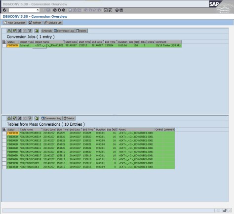
Figure 8-114 Report DB6CONV: Successfully finished conversion job
Considerations for InfoCube conversions
DB6CONV provides options for excluding tables that are contained in conversion jobs from actually being converted. It is best not to use the options to exclude tables to make sure that all tables belonging to an InfoCube are converted.
When a conversion aborts, take the following actions:
1. For each table that failed during the conversion, examine the conversion log to identify the root cause of the failure. If the root cause is the issue described in “Known issue with InfoCube conversions” on page 376, apply the fix or the workaround and continue with the next step. If the issue is not listed, open an incident at SAP.
2. Reset the conversion of each table that failed in the Table from Mass Conversions area in the Conversion Overview window.
3. Reset the conversion of the whole job in the Conversion Jobs area.
4. Go back to the SAP_CDE_CONVERSION_DB6 report, reselect the InfoCube or all InfoCubes and create another conversion job. This new job contains only the tables that failed or have not yet been processed.
5. Schedule and run the new conversion job.
Known issue with InfoCube conversions
When you convert column-organized tables to row-organized, the row-organized tables are not compressed. The compression options in the job details window cannot be changed to row or adaptive compression and the default option, KEEP, is not applied correctly. This issue can be corrected by activating compression using the DB6CONV report. Make sure that you have installed the most recent version of DB6CONV.
8.7 Deployment
DB2 Cancun Release 10.5.0.4 brings a lot of improvements and enables additional features. This makes it a preferred release, especially for new deployments. To get your SAP BW system ready for using BLU Acceleration, three options are available:
•If your SAP BW system runs on DB2 but currently uses DB2 10.1 or earlier, use these steps:
a. Upgrade your DB2 database to DB2 10.5 as described in the SAP database upgrade guide (Upgrading to Version 10.5 of IBM DB2 for Linux, UNIX, and Windows5).
This guide is at the SAP Service Marketplace:
Select Database Upgrades → DB2 UDB.
b. Adapt your DB2 parameter settings (as described in SAP Note 1851832), including the parameter settings for BLU Acceleration that are described in the “DB2 Column-Organized Tables (BLU Acceleration)” section of SAP Note 1851832.
c. Install the required Support Packages and SAP Kernel described in chapter 8.2, “Prerequisites and restrictions for using BLU Acceleration in SAP BW” on page 255.
d. Install the required code corrections described in chapter 8.2, “Prerequisites and restrictions for using BLU Acceleration in SAP BW” on page 255.
e. Configure the SAP BW system for DB2 BLU Acceleration by setting the RSADMIN parameters.
•If you want to install a completely new SAP BW system, use these steps:
a. Install the system directly on DB2 10.5 with the SAP Software Logistics (SL) Toolset. Be sure to use the most recent release and Support Package Stack.
b. Adapt the DB2 parameter settings manually as described in the DB2 Column-Organized Tables (BLU Acceleration) section of SAP Note 1851832.
c. If necessary, upgrade to the required Support Packages and SAP Kernel (see 8.2, “Prerequisites and restrictions for using BLU Acceleration in SAP BW” on page 255).
d. Install the required code corrections described in chapter 8.2, “Prerequisites and restrictions for using BLU Acceleration in SAP BW” on page 255.
e. Configure the SAP BW system for DB2 BLU Acceleration by setting the RSADMIN parameters.
•If you have an SAP BW system that runs on DB2 or another database platform supported by SAP and you want to create a new BW system by performing a heterogeneous system copy (migration) of the existing system, proceed as follows:
a. Upgrade your existing system to the required Support Package level and SAP kernel version (see 8.2, “Prerequisites and restrictions for using BLU Acceleration in SAP BW” on page 255).
b. Install the required code corrections described in chapter 8.2, “Prerequisites and restrictions for using BLU Acceleration in SAP BW” on page 255.
c. Generate the DDL for the SAP BW tables for the target DB2 database with the SMIGR_CREATE_DDL report. In this step, you can either select to directly generate DDL for creating column-organized tables or you can choose row-organized tables and convert selected SAP BW objects to BLU Acceleration later in the target system.
d. Perform the heterogeneous system copy as described in the SAP documentation and install the target system directly on DB2 10.5.
e. Before you start loading the data into the target system, adapt the DB2 parameter settings manually as described in the DB2 Column-Organized Tables (BLU Acceleration) section of SAP Note 1851832.
f. Configure the SAP BW system for DB2 BLU Acceleration by setting RSADMIN parameters.
g. Perform the required post migration steps including the execution of the RS_BW_POST_MIGRATION report in the target system.
8.7.1 Upgrading an SAP BW system to DB2 10.5
The procedure to upgrade an SAP database to DB2 10.5 is described in the SAP database upgrade guide (Upgrading to Version 10.5 of IBM DB2 for Linux, UNIX, and Windows). This is mentioned in 8.7, “Deployment” on page 376.
After you have performed the database upgrade and before you start to create BLU Acceleration InfoCubes or convert existing InfoCubes to column-organized tables, you must set the DB2 configuration parameters to the recommended values for BLU Acceleration of SAP Note 1851832 manually and restart the DB2 instance.
The most important configuration parameter settings for BLU Acceleration that are described in SAP Note 1851832 are as follows:
•Database Manager configuration parameters
– INTRA_PARALLEL = YES
– MAX_QUERYDEGREE = ANY
•Database configuration parameters
– INSTANCE_MEMORY >= 64 GB
– DATABASE_MEMORY = AUTOMATIC
– SHEAPTHRES_SHR = 40% of the instance memory
– SORTHEAP = 1/20 of SHEAPTHRES_SHR
– UTIL_HEAP_SZ = AUTOMATIC
•Buffer pool size = 40% of instance memory
•To benefit from the parallel processing capabilities of BLU Acceleration, at least eight processor cores are needed.
The ratio of 8 GB RAM per processor core ensures a high performance on larger systems as well. Development or quality assurance systems with a minor amount of parallel workload are able to use the parallel processing capabilities of BLU Acceleration with at least four processor cores and 32 GB RAM.
If you want to create SAP BW temporary tables, PSA tables, and InfoObject tables as column-organized tables, you must set the RSADMIN parameters shown in Table 8-7 with report SAP_RSADMIN_MAINTAIN.
Table 8-7 SAP BW RSADMIN parameters for DB2 BLU Acceleration
|
RSADMIN Parameter Name and Value
|
Comment
|
|
DB6_IOBJ_USE_CDE=YES
|
Create SID and time-independent and time-dependent attribute SID tables of new characteristic InfoObjects as column organized tables
|
|
DB6_PSA_USE_CDE=YES
|
Create new PSA tables as column-organized tables
|
|
DB6_TMP_USE_CDE=YES
|
Create new BW temporary tables as column-organized tables
|
Make sure that you have implemented the latest version of SAP Note 1152411 for the SAP DBA Cockpit. Then create at least one BLU table in your system, for example by creating a new column-organized InfoCube.
After these steps run the latest available version (at least V44) of the db6_update_db script. The script checks whether at least one BLU table exists. If this is the case it deletes the SAP specific Workload Manage (WLM) service classes and workloads and sets a WLM threshold is set for the number of long running BW queries on BLU that can be executed in parallel. With this threshold you avoid overloading the CPU resources of the database server. The most recent version of the script is in the attachment of SAP Note 1365982 in the “DB6: Current db6_update_db/db2_update_client Script (V45)”. The version number changes over time.
8.7.2 Installing a new SAP BW system on DB2 10.5
The installation of a new SAP BW system does not involve the creation of InfoCubes or other SAP BW objects. Before you start creating BW objects that use column-organized tables, proceed by setting the DB2 configuration parameters as it is done during an update process, make sure that the SAP DBA Cockpit is up to date, create at least one BLU table and run the db6_update_db script. These steps are described in 8.7.1, “Upgrading an SAP BW system to DB2 10.5” on page 378.
If you want to create SAP BW temporary tables, PSA tables, and InfoObject tables as column-organized tables you must set the RSADMIN parameters shown in Table 8-7 with report SAP_RSADMIN_MAINTAIN.
8.7.3 Migrating an SAP BW system to DB2 10.5 with BLU Acceleration InfoCubes
The procedure to perform a heterogeneous system copy (also called migration) of an SAP NetWeaver system is described in the SAP system copy guide that is available on SAP Service Marketplace:
Select <Your SAP NetWeaver Main Release> → Installation.
With SAP Note 1969500, you have two options when you perform an SAP heterogeneous system copy. You can choose whether you want to migrate your InfoCubes only or all BW objects for which BLU Acceleration is supported to column-organized tables. This works when your SAP BW system already runs on DB2 or when you migrate your SAP BW system from another database platform to DB2.
Figure 8-115 shows the steps for the source system and the target system that must be completed during a heterogeneous system copy of an SAP BW system.

Figure 8-115 Steps to perform an SAP BW heterogeneous system copy
The steps in the red boxes are specific to SAP BW systems. The most important step to ensure that BW object tables are created as column-organized tables in the target system is “Create DDL for Target DB.” In this step, you run the SMIGR_CREATE_DDL report on the source system to generate DDL statements for creating tables and indexes for SAP BW objects in the target database.
With SAP Note 1969500, two new options for creating DDL for column-organized tables are available in the report.
Complete these steps to create the DDL files needed for the migration:
1. Run the SMIGR_CREATE_DDL report in SAP transaction SE38.

Figure 8-116 Report SMIGR_CREATE_DDL: main window
The Database Version field provides the following options:
– When your source system runs on DB2, the options shown in Figure 8-117 are offered.

Figure 8-117 DB2 feature options for a heterogeneous system copy of an SAP BW system that runs on DB2
The options are as follows:
• Keep Source Settings: The report generates the same DDL for the target database that is used in the source database.
• Use BW Basic Table Layout: The report generates DDL without MDC and DDL for row-organized tables only.
• Use Multi-Dimensional Clustering (MDC) for BW: The report generates DDL with MDC for all PSA tables, DSO change log tables, DSO activation queue tables, F fact tables, E fact tables that already use MDC in the source system, and DSO active tables that already use MDC in the source system.
• Use Column-Organized Tables for BW InfoCubes: The report generates DDL for column-organized tables for the InfoCube fact tables and dimension tables. For the other SAP BW object tables, it generates DDL with MDC if possible.
• Use Column-Organized Tables for all BW Objects: The report generates DDL for column-organized tables for InfoCube fact tables, InfoCube dimension tables, DSO active tables, PSA tables, and InfoObject SID and attribute SID tables. For the other SAP BW object tables, it generates DDL with MDC if possible.
– If your source system runs on another database platform, the options shown in Figure 8-118 are offered.

Figure 8-118 DB2 feature options for a heterogeneous system copy of an SAP BW system that runs on another database platform
The options are as follows:
• Use BW Basic Table: The report generates DDL without MDC and DDL for row-organized tables only.
• Use Multi-Dimensional Clustering (MDC) for BW: The report generates DDL with MDC for all PSA tables, DSO change log tables, DSO activation queue tables, F fact tables, E fact tables that use range partitioning in the source system, and DSO active tables that use range partitioning in the source system.
• Use Column-Organized Tables for BW InfoCubes: The report generates DDL for column-organized tables for the InfoCube fact tables and dimension tables. For the other SAP BW object tables, it generates DDL with MDC if possible.
• Use Column-Organized Tables for all BW Objects: The report generates DDL for column-organized tables for InfoCube fact tables, InfoCube dimension tables, DSO active tables, PSA tables, and InfoObject SID and attribute SID tables. For the other SAP BW object tables, it generates DDL with MDC if possible.
3. Choose Use Column-Organized Tables for all BW Objects, select the output directory for the generated DDL in the Installation Directory field, and run the report (Figure 8-119).

Figure 8-119 Report SMIGR_CREATE_DDL: Generating DDL for column-organized tables
When the report is finished, the success message is shown (Figure 8-120).

Figure 8-120 Report SMIGR_CREATE_DDL: Final message when completed
4. In the directory that you entered in Installation Directory, locate these files:
– Generated DDL
– The *.LST file that contains the list of the files that the report created
The db6_compression_tablist.txt file is generated only when the source system runs on DB2. This file contains the compressed row-organized tables and the row compression type (static or adaptive) that is used. You can use this file as input when you generate and load your DB2 target database to compress the tables in exactly the same way as in the source database.

Figure 8-121 Directory with the sample files generated by report SMIGR_CREATE_DDL
The SMIGR_CREATE_DDL report generates a *.SQL file for each SAP data class that contains at least one table with DB2-specific features such as MDC, distribution keys, clustered indexes, or column-organized tables.
5. During the installation of the target system, the SAP installation tool asks for the location of the files. Make sure that the files are accessible.
Example 8-13 shows output of the SMIGR_CREATE_DDL report for the E fact table, /BIC/EROWCUBE1, of a row-organized InfoCube that is to be created with column-organized tables in the target system. A tab entry is for the table itself, several ind entries are for the indexes that exist on the row-organized table in the source system.
The entries for most of the indexes, for example, /BIC/EROWCUBE1~020, contain no SQL statement because these indexes are not created in the target database. The entry for index /BIC/EROWCUBE1~P contains an ALTER TABLE ADD CONSTRAINT statement that must be used for column-organized tables.
Example 8-13 Sample output of report SMIGR_CREATE_DDL
tab: /BIC/EROWCUBE1
sql: CREATE TABLE "/BIC/EROWCUBE1"
("KEY_ROWCUBE1P" INTEGER
DEFAULT 0 NOT NULL,
"KEY_ROWCUBE1T" INTEGER
DEFAULT 0 NOT NULL,
"KEY_ROWCUBE1U" INTEGER
DEFAULT 0 NOT NULL,
"KEY_ROWCUBE11" INTEGER
DEFAULT 0 NOT NULL,
"KEY_ROWCUBE12" INTEGER
DEFAULT 0 NOT NULL,
"KEY_ROWCUBE13" INTEGER
DEFAULT 0 NOT NULL,
"KEY_ROWCUBE14" INTEGER
DEFAULT 0 NOT NULL,
"KEY_ROWCUBE15" INTEGER
DEFAULT 0 NOT NULL,
"SID_0CALMONTH" INTEGER
DEFAULT 0 NOT NULL,
"/B49/S_CRMEM_CST" DECIMAL(000017,000002)
DEFAULT 0 NOT NULL,
"/B49/S_CRMEM_QTY" DECIMAL(000017,000003)
DEFAULT 0 NOT NULL,
"/B49/S_CRMEM_VAL" DECIMAL(000017,000002)
DEFAULT 0 NOT NULL,
"/B49/S_INCORDCST" DECIMAL(000017,000002)
DEFAULT 0 NOT NULL,
"/B49/S_INCORDQTY" DECIMAL(000017,000003)
DEFAULT 0 NOT NULL,
"/B49/S_INCORDVAL" DECIMAL(000017,000002)
DEFAULT 0 NOT NULL,
"/B49/S_INVCD_CST" DECIMAL(000017,000002)
DEFAULT 0 NOT NULL,
"/B49/S_INVCD_QTY" DECIMAL(000017,000003)
DEFAULT 0 NOT NULL,
"/B49/S_INVCD_VAL" DECIMAL(000017,000002)
DEFAULT 0 NOT NULL,
"/B49/S_OPORDQTYB" DECIMAL(000017,000003)
DEFAULT 0 NOT NULL,
"/B49/S_OPORDVALS" DECIMAL(000017,000002)
DEFAULT 0 NOT NULL,
"/B49/S_ORD_ITEMS" DECIMAL(000017,000003)
DEFAULT 0 NOT NULL,
"/B49/S_RTNSCST" DECIMAL(000017,000002)
DEFAULT 0 NOT NULL,
"/B49/S_RTNSQTY" DECIMAL(000017,000003)
DEFAULT 0 NOT NULL,
"/B49/S_RTNSVAL" DECIMAL(000017,000002)
DEFAULT 0 NOT NULL,
"/B49/S_RTNS_ITEM" DECIMAL(000017,000003)
DEFAULT 0 NOT NULL)
IN "&location&"
INDEX IN "&locationI&"
LONG IN "&locationL&"
DISTRIBUTE BY HASH (
"KEY_ROWCUBE11"
, "KEY_ROWCUBE12"
, "KEY_ROWCUBE13"
, "KEY_ROWCUBE14"
, "KEY_ROWCUBE15"
, "KEY_ROWCUBE1T"
, "KEY_ROWCUBE1U"
)
ORGANIZE BY COLUMN;
ind: /BIC/EROWCUBE1~0
ind: /BIC/EROWCUBE1~020
ind: /BIC/EROWCUBE1~040
ind: /BIC/EROWCUBE1~050
ind: /BIC/EROWCUBE1~060
ind: /BIC/EROWCUBE1~070
ind: /BIC/EROWCUBE1~080
ind: /BIC/EROWCUBE1~P
sql: ALTER TABLE "/BIC/EROWCUBE1"
ADD CONSTRAINT "/BIC/EROWCUBE1~P" unique
("KEY_ROWCUBE1T",
"KEY_ROWCUBE11",
"KEY_ROWCUBE12",
"KEY_ROWCUBE13",
"KEY_ROWCUBE14",
"KEY_ROWCUBE15",
"KEY_ROWCUBE1U",
"KEY_ROWCUBE1P");
6. Before you start to load the database, set the DB2 configuration parameters as described in 8.7.1, “Upgrading an SAP BW system to DB2 10.5” on page 378.
7. After you have installed the target database, created the tables, and loaded the data, you will have BLU tables in the database.
8. Make sure that you have implemented the latest version of SAP Note 1152411 for the SAP DBA Cockpit.
9. Run the latest available version (at least V44) of the db6_update_db script. The script checks whether at least one BLU table exists. If this is the case it deletes the SAP specific service classes and workloads and sets a WLM threshold is set for the number of long running BW queries on BLU that can be executed in parallel. With this threshold you avoid overloading the CPU resources of the database server. The most recent version of the script is in the attachment of SAP Note 1365982 in the “DB6: Current db6_update_db/db2_update_client Script (V45)”. The version number changes over time.
10. If you want to create SAP BW temporary tables, PSA tables, and InfoObject tables as column-organized tables you must set the RSADMIN parameters shown in Table 8-7 with report SAP_RSADMIN_MAINTAIN.
11. Run the RS_BW_POST_MIGRATION report to complete the migration of the SAP BW object tables.
8.8 Performance of SAP BW with BLU Acceleration
This section describes the performance benefits of BLU Acceleration in an SAP BW environment. An internal lab test is used for illustration purposes. This test is based on a performance test scenario adopted to meet the characteristics observed in customer scenarios as closely as possible. By this example, the most important attributes of the column-store implementation are highlighted, which have a significant effect as to improved performance, reduced resource consumption, and enhanced usability.
8.8.1 Example environment
The starting point for these measurements is a basic cumulative InfoCube that is provided by the performance test. This InfoCube references 75 characteristics, in total. Those characteristics are spread on 16 dimensions. Each dimension holds 2 - 11 characteristics. This InfoCube definition is copied three times: once using MDC as a clustering method and twice using Organized in Columns to create a standard and a flat InfoCube.
Preparation
The data used to load the InfoCubes for this scenario is generated. The data produced by the generator represents transactional data of five years. This data is stored in plain text files containing 108 rows in total. These files are loaded to a PSA, which in turn represents the source for Data Transfer Processes (DTPs) that load the data into the InfoCubes.
As a result, both InfoCubes are loaded with exactly the same data. The fact tables of each InfoCube contain 108 rows. The cardinality of the resulting dimension tables varies between a few hundred and 11*106 rows, depending on the number of characteristics and their cardinality. The dimensions, grouped by their cardinality, are distributed in the following way:
•Six small dimensions contain less than 10,000 rows.
•Four medium dimensions contain more than 10,000 but less than 100,000 rows.
•Six large dimensions contain more than 100,000 records.
From the application server point of view, the process of creating a column-organized InfoCube using BLU Acceleration is nearly the same as creating one in the row store. See “Table layout of column-organized InfoCubes” on page 279. A flat InfoCube is created as described in 8.5.2, “Flat InfoCubes in SAP BW 7.40” on page 297. The load process is exactly the same. A common runtime layer for both data stores enables DB2 to provide a transparent interface to the application. After a table is created using BLU Acceleration, it is accessed in the same way as a conventional table. This brings two fundamental benefits compared to less integrated architectures:
•Existing programs and processes need no, or only minimal, adoptions to use BLU Acceleration.
•Column- and row-organized InfoObjects can coexist without any special treatment within the application allowing an easy migration to BLU Acceleration.
Configuration
The hardware used for these query measurements is an IBM Power 770. A logical partition (LPAR) is configured with eight Power7 cores at 3.1 GHz each and 64 GB of RAM running AIX 7.1. This LPAR runs both, the SAP BW application server and the DB2 Cancun Release 10.5.0.4database server. An IBM XIV is used as storage system.
These measurements aim for a direct comparison of row and column store within the same database instance. For that reason, a common configuration is used, which fits to columnar stored objects and to objects in the row store. Because this lab configuration is a two-tier setup, the database cannot dispose of the RAM completely. Instead, 9 GB of RAM are reserved for the operating system and the application server. The remaining 55 GB of RAM are assigned to the database server.
The database memory is mainly consumed by two memory areas: the buffer pool and the sort heap threshold for shared sorts. Each is set to 22 GB. The utility heap size and the sort heap size for private sorts are set to 2 GB. Intrapartition parallelism is enabled with unlimited maximum degree (according to the recommendations in 8.7.1, “Upgrading an SAP BW system to DB2 10.5” on page 378).
Additional configuration for BLU Acceleration is not required. Because BLU Acceleration is a memory-optimized, but not an in-memory column store technology, it uses data pages to organize and buffer data, just as the conventional row store does. This architectural approach has several advantages, including these:
•Neither a table, nor even column has to fit completely into RAM. Frequently used pages reside in buffer pools and less frequently used ones can be dynamically read from disk. Thus table and column sizes are not limited by the available amount of RAM.
•DB2 is able to share buffers between both data stores. This simplifies the configuration because no additional parameters have to be maintained. Furthermore, it reduces the over provisioning needed to cope with peak high load phases.
8.8.2 Storage consumption and compression rates
To make a statement on relative storage consumptions or compression rates, a reference size is required. Both the row store and column store use compression techniques, but differ from each other in terms of indexes and constraints. As a consequence, a direct comparison is not meaningful.
Therefore, both storage saving mechanisms and the impact of the denormalization of the flat InfoCube must be compared against a neutral element. However, in each case, the storage actually used by tables and indexes must be considered separately. For that purpose, a fourth, uncompressed instance of the InfoCube is created.
Regarding compression and storage type, there are now four differently configured cubes:
ROW uncompressed No compression technique is used.
ROW compressed Page level compression, adaptive compression, and index compression are used.
BLU Acceleration On column-organized tables, a new, order-preserving compression algorithm is activated and maintained automatically.
Flat InfoCube The same attributes as for the BLU accelerated standard InfoCube apply, because this InfoProvider is only available with BLU Acceleration.
Table 8-8 lists the actual storage consumptions of the cubes. For each cube, the total consumption is horizontally split into the size of fact and dimension tables. Vertically, the consumption is split into storage consumed by actual table data and storage consumed by indexes and similar structures.
Table 8-8 Storage consumption of InfoCube objects split up into their components
|
|
|
Fact table
|
Dimension tables
|
Total
|
|
ROW uncompressed
|
42.23 GB
|
3.19 GB
|
46.42 GB
|
|
|
|
Tables
|
32.47 GB
|
0.93 GB
|
33.40 GB
|
|
|
Indexes
|
10.77 GB
|
2.26 GB
|
13.03 GB
|
|
ROW compressed
|
17.50 GB
|
1.99 GB
|
19.34 GB
|
|
|
|
Tables
|
11.02 GB
|
0.49 GB
|
11.50 GB
|
|
|
Indexes
|
6.33 GB
|
1.51 GB
|
7.83 GB
|
|
BLU Acceleration
|
4.99 GB
|
1.16 GB
|
6.15 GB
|
|
|
|
Tables
|
4.97 GB
|
0.15 GB
|
5.12 GB
|
|
|
Indexes
|
0.01 GB
|
1.01 GB
|
1.02 GB
|
|
|
Synopsis
|
0.01 GB
|
0.00 GB
|
0.01 GB
|
|
Flat InfoCube
|
5.59 GB
|
0.00 GB
|
5.59 GB
|
|
|
|
Tables
|
5.57 GB
|
0.00 GB
|
5.57 GB
|
|
|
Indexes
|
0.01 GB
|
0.00 GB
|
0.01 GB
|
|
|
Synopsis
|
0.01 GB
|
0.00 GB
|
0.01 GB
|
In total, conventional compression methods on the row store reduce the total storage consumption by a factor of 2.4x. Using BLU Acceleration, this ratio is increased to a factor of 7.5x. In case of the flat InfoCube, the data volume is reduced by even factor 8.3.
Comparing the compression rates of fact and dimension tables, the compression rate on the row store is constant on both table types. The column-organized tables, however, in total vary in their compression rate depending on their type. The fact table reaches a compression rate of 8.5x but the dimension tables are compressed by factor 2.8x.
On closer consideration of the dimension tables, actual table and index sizes, their ratio attracts attention. The indexes are by factors larger than the actual data. This also applies to the uncompressed InfoCube. Thus, this fact does not result from compression. The reason is that for dimension tables in the row store, an index is defined on each column. The data is actually stored twice, in the table and in the index as well. In addition, the index tree needs some storage, too, which makes this ratio reasonable. In the case of column-organized dimension tables, only two constraints are defined: The primary key constrained on the dimension identifier column, and a unique key constrained on all columns. The second one represents a unique index. According to that, a ratio of index and table size larger than one in the column store is also reasonable.
Although the compressed indexes on the columnar dimension tables are already 1.2 times smaller than those of the row-based tables, the actual data in the columnar dimension tables is still 6.7 times smaller than their own indexes. This is because indexes, in general, are more difficult to compress than data. In this particular case, the index compression rate on column-organized tables is already high. Because of the advantages of a column store regarding compression capabilities and the new compression algorithm used by BLU Acceleration, the data compression is even better.
The effect of the increased redundancy of the flat InfoCube data, caused by the denormalization of the enhanced star schema, is far smaller than the benefit gained by abandoning the indexes on dimension tables and dropping the SID columns required for modeling the foreign key relationship. This makes the flat InfoCube even more space efficient than the standard InfoCube with BLU Acceleration.
In summary, the following statements can be made:
•With the use of BLU Acceleration, a compression rate of 7.5x is reached in this test scenario.
•The new flat InfoCube with BLU Acceleration even reaches a compression rate of 8.3x.
•Even compared to the most sophisticated row-based compression features, the storage consumption can be reduced by 3.2-3.5x because of the advanced possibilities of the new columnar compression algorithm.
•Assuming that dimension tables in the field have a cardinality of less than 10% of the number of fact table entries, even higher compression rates of InfoCubes are possible.
8.8.3 Query performance
To make a general assumption about the query performance of SAP BW using DB2 BLU Acceleration, a set of queries is used that satisfy several attributes.
The queries differ from each other in the following terms:
•The queries select either 20% or 40% of the transactional data.
•The predicate is either a range predicate on the time dimension, an access using a hierarchy, a predicate on a user defined dimension.
•Three different user defined dimensions are used: A small one with 10^6 rows, a medium one with 6*10^6 rows and a large one with 11*10^6 rows.
•There are three kinds of predicates defined on these user defined dimensions: Range predicates, lists, or they are accessed using temporary tables which are created for predicates including a large list.
This results in a set of 22 queries. For simplicity, the queries are labeled from 1 to 22, based on the order of the attributes. The SAP Business Explorer (BEx) Query Designer is used to define these queries as BEx queries, which form the basic instrument to query SAP BW data.
These BEx queries are designed to compare database performance only. Therefore, the OLAP cache is deactivated during the measurements. So the query processing almost exclusively occurs on the database server. This also ensures that no precalculated results are used.
By shifting the workload from the application server to the database, the effect on the query performances by running the application server on the same LPAR as the database server is minimized also, because the application server is nearly idle while the queries are run.
The database is configured to provide enough memory for the buffer pool so that each InfoCubes and temporary results completely fit into memory. All queries are run twice, recording only the second result to make sure that no I/O effects are distorting the result. This approach ensures reproducible results by eliminating I/O, a hardly predictable factor, which has a great influence on database performance. Furthermore, it assures that query processing on both technologies, the conventional row store, and BLU Acceleration, are compared under the same conditions.
However, two important advantages of BLU Acceleration are implicitly left out by these measurements:
•BLU Acceleration provides far better compression capabilities than the row store. As a result, I/O costs and the amount of buffer pool memory that is required to buffer data are reduced. To make the row-based tables fit into the buffer pool, more memory must be provided than the tables with BLU Acceleration require.
•By using BLU Acceleration, only the data that is actually used by the query must be read. Columns that are not required to execute the query are never read.
As a consequence, these measurements compare pure processing time only. The results of these measurements are outlined in Figure 8-122.

Figure 8-122 Query performance results comparing conventional row store performance with queries using BLU Acceleration
On average, BLU Acceleration on a standard InfoCube outperforms the row-based sample queries by factor 6.9x. On a flat InfoCube, BLU Acceleration is even 20.6x faster on average than a standard row-based InfoCube. The ratio varies depending on the query attributes from 2x to 55x. Customers report an even larger performance gain by using BLU Acceleration on real life data.
Scalability and throughput
Besides the static analysis of single query performance, scalability of BLU Acceleration is also investigated. For that purpose, scalability is analyzed in two dimensions:
•A growing amount of analyzed data
•An increasing number of parallel running queries
Starting with the performance behavior caused by a growing amount of data, a single query is chosen as a starting point. The query is modified to fetch data starting from 0% up to 100% of the InfoCube. The resulting 21 queries are used to make a prediction on the engine’s scalability.
The run times that are achieved in this test are shown in Figure 8-123. Besides the actual measured points, this chart shows linear approximations of both measurement series. The row store and BLU Acceleration show an almost linear scaling behavior. The obvious performance advantage through BLU Acceleration makes it hard to show this linearity in the chart. A detailed analysis of the measured run times shows a similarly low deviation from the approximation as the measurements on the row store do.

Figure 8-123 Performance scalability regarding the amount of selected data
To measure parallel query throughput, some additional aspects must be considered. Especially synergy effects between queries should be minimized. For that purpose, the following setup is used:
•Eight InfoCubes are set up as data source for the queries.
•Up to 24 query sets are run against each cube in parallel.
•Each of those sets contains the same queries but in different order.
In an environment where multiple queries are run in parallel, not all data is expected to be in the buffer pool. Thus the buffer pool is configured to provide only enough memory for one-third of the actual size all InfoCubes would need in total.
The first measurement with only one query set running at a time forms a reference. In further measurements up to 192 query sets are run against all eight cubes in parallel.
All query sets are run several times in a loop. The first and the last iterations are dropped in each case. By taking the run times of the remaining iterations, an average throughput can be computed, which describes how many queries can be run per hour. These results are outlined in Figure 8-124.

Figure 8-124 Average query throughput of parallel running queries
The results show that the actual throughput is slightly increasing. Monitoring the operating system when the tests are running shows a CPU utilization around 90% in all cases. So, at least three interpretations can be derived from these observations:
•The parallel processing of SAP BW queries using BLU Acceleration is capable of utilizing almost all available processors.
•Even if multiple queries run in parallel and the available resources must be shared, the throughput remains constant.
•The system remains responsive, even under a high, parallel workload.
In summary, both tests show that DB2 with BLU Acceleration scales well regarding a growing amount of data and with an increasing degree of parallelism. The linear scaling behavior with an increasing data volume results from the optimized parallel query processing, which allows a high utilization of available resources. Furthermore, from the use of SIMD instructions, the parallel processing within a process is supported, additionally. At the same time, a high cache utilization is reached, which enables the processor to keep fully utilized and reduces the number of context switches. This makes BLU Acceleration stable in terms of parallel workload.
Access plans
Performance reliability and stability depend significantly on access plans that are generated by the query optimizer. During query compilation time, the optimizer must make decisions on join order, join types and which indexes are to be used.
The waiver of explicit indexes and several join types using BLU Acceleration reduces the degree of freedom for possible decisions of the optimizer and thus increases the reliability of access plans. Accessing dimension tables using a full table scan instead of an index scan is accelerated in several ways.
Synopsis tables hold additional information about sets of tuples, describing per column which value ranges are included. This supports skipping complete sets of tuples if the searched value is not included. In contrast to indexes, synopsis tables are created automatically. In addition, actionable compression allows scanning the table without having to decompress it first. This does not only save memory but also computing time and enables DB2 to compare more values immediately by using SIMD instructions.
Example 8-14 shows two excerpts of access plans joining a dimension table to a fact table. The left is an example using the conventional row store; the right is an example using BLU Acceleration. As this example shows, column-organized tables are labeled as CO-TABLE. Data skipping is applied implicitly by the table scan operator. Therefore, it is not mentioned separately.
Example 8-14 Excerpts of access plans joining a dimension table to the fact table compare conventional row store to BLU Acceleration
[upper part of the access plan skipped in the intrests of clarity]
Conventional row store: BLU Acceleration:
9.48521e+07 9.47975e+07
^HSJOIN ^HSJOIN
( 12) ( 10)
2.61552e+06 1.23391e+06
721997 31872
/------+------- /-------+-------
1e+08 1731 1e+08 1731
TBSCAN FETCH TBSCAN TBSCAN
( 13) ( 14) ( 11) ( 12)
2.60943e+06 36.5425 1.23279e+06 59.1637
721992 5 31863.5 8.52632
| /---+---- | |
1e+08 1826 1826 1e+08 1826
TABLE: SAPBL2 IXSCAN TABLE: SAPBL2 CO-TABLE: SAPBL2 CO-TABLE: SAPBL2
/BIC/FICROW02 ( 15) /BIC/DICROW02T /BIC/FICBLU02 /BIC/DICBLU02T
Q4 14.7311 Q6 Q2 Q4
2
|
1826
INDEX: SAPBL2
/BIC/DICROW02T~0
Q6
8.8.4 Discussion
As outlined by the tests in the previous sections, SAP BW InfoCubes on DB2 with BLU Acceleration outperform conventional row-based InfoCubes regarding storage consumption and query performance.
Additional internal lab tests (not outlined in this document) show a comparable ETL performance. The compression rate of 8.3x is by factor of 3.5x better than on the row store. Even running completely in memory, the query performance is up to 22x better. With I/O involved, even higher ratios are expected because of the storage model.
BLU Acceleration is a true column store. That means the complete internal representation and the engine internal processing is columnar. Other column-oriented storage models, which do not use an in-memory architecture, such as Decomposition Storage Model (DSM)6 and Partition Attributes Across (PAX)6 are easy to implement into an existing engine, but their architectures have some major drawbacks (see Table 8-9).
Table 8-9 Storage model comparison
|
|
NSM1
|
DSM
|
PAX
|
BLU Acceleration
|
|
Spatial locality
|
|
X
|
X
|
X
|
|
Cheap record construction
|
X
|
|
X
|
X
|
|
I/O Avoidance
|
|
X2
|
|
X
|
1 N-ary Storage Model (NSM)/row store
2 Additional I/O to fetch row key
DSM is basically a row store with an extended implementation of vertical partitioning. PAX organizes data in column-oriented style at page level only. In this way, a cache pollution can be admittedly reduced, SIMD instructions can be applied and records cheaply reconstructed, but nevertheless all data must be read to process a query referencing the table.
BLU Acceleration stores columns on separate pages. This allows you to read only the columns that are actually needed. Regarding InfoCubes, that data store design implies that adding key figures to an InfoCube does not affect the performance of existing queries. Furthermore, spatial locality of data and subsequently cache utilization and SIMD exploitation are maximized. Both play an important role in calculating aggregates and filtering selected dimension entries. Furthermore this enables DB2 Cancun Release 10.5.0.4 to support flat InfoCubes, because the large number of columns in the fact table has no negative impact on the I/O performance.
8.9 BLU Acceleration for SAP near-line storage solution on DB2 (NLS)
The SAP near-line storage solution on DB2 (NLS) has been enhanced so that tables for the NLS storage objects can be created as column-organized tables. Table 8-10 lists the supported SAP NetWeaver releases and SAP BW Support Packages. See SAP Note 1834310 before you use this feature with NLS. For DB2 Cancun Release 10.5.0.4 specific enhancements read SAP Note 2030925.
Table 8-10 Supported SAP BW releases and support packages
|
SAP NetWeaver release
|
Minimum BW Support Packages1
|
Recommended BW Support Package
|
|
7.01
|
6
|
15
|
|
7.02
|
3
|
15
|
|
7.30
|
1
|
11
|
|
7.31
|
1
|
10
|
|
7.40
|
GA
|
5
|
1 These BW Support packages additionally require the installation of SAP Note 1834310
8.9.1 Overview of NLS
NLS is a category of data persistency that is similar to archiving. Using an NLS database enables you to transfer historical read-only data of the InfoProviders from an SAP BW system to a separate NLS database. The data in the NLS database can be accessed transparently from an SAP BW system.
Figure 8-125 shows a basic setup of the NLS solution with DB2 for Linux, UNIX, and Windows as an NLS database. This is an excerpt from SAP Guide: Enabling SAP NetWeaver Business Warehouse Systems to Use IBM DB2 for Linux, UNIX, and Windows as Near-Line Storage (NLS):
Select <Your SAP NetWeaver Main Release> → Operations → Database-Specific Guides.
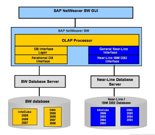
Figure 8-125 Basic Setup of NLS solution
Mainly, two data models are implemented on the NLS database on DB2 to store historical read-only data; decisions about the data models are based on whether the InfoProvider is similar to an InfoCube object or a DataStore object.
InfoCube objects that are created in the NLS database contain the following tables:
•Archiving request table to store the archiving request information
•Fact tables that store the key figures of the original InfoCube
•A set of dimension tables to store the characteristics of the original InfoCube
The DataStore object created in the NLS database contains the following items:
•NLS archiving request table to store the archiving request information
•NLS active data table to store the business-related information of the original DataStore object
These tables are created on the NLS database when you create a data archiving process for an InfoProvider on your SAP BW system.
8.9.2 BLU Acceleration for NLS storage objects
By default, the data on NLS databases is stored in row-organized tables. If your NLS database runs on DB2 10.5, you can choose to create these tables as column-organized tables. DB2 column-organized tables support the objects of both the NLS InfoCubes and DataStore data models.
To use column-organized tables, you must set the RSADMIN parameter DB6_NLS_USE_CDE to YES in your SAP BW system. This parameter is disabled by default. If you create a new data archiving process for an InfoProvider with this parameter enabled, the corresponding new tables in the NLS database are created as column-organized tables. This parameter has no impact on existing row-organized tables in the NLS database.
The following procedure outlines how to set the DB6_NLS_USE_CDE parameter and how to create column-organized tables for NLS InfoCubes and DataStore objects:
1. In your SAP BW system, call transaction SE38 and run the SAP_RSADMIN_MAINTAIN report.
2. In the Object field, enter DB6_NLS_USE_CDE. In the Value field, enter YES. Select the INSERT option and click the Execute icon (Figure 8-126).

Figure 8-126 Report SAP_RSADMIN_MAINTAIN: Set DB6_NLS_USE_CDE parameter
3. Select an InfoProvider and then select Create Data Archiving Process (Figure 8-127). In this example, InfoCube /BIB/Bench02 was selected as InfoProvider.
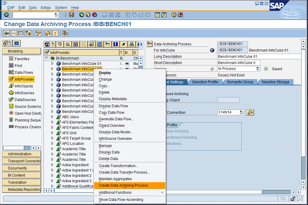
Figure 8-127 SAP Data Warehousing Workbench: creating data archiving process
4. On the General Settings tab (Figure 8-128), proceed as follows:
a. For the Data Archiving Process, enter descriptions in the Long Description and Short Description fields.
b. Deselect ADK-Based Archiving if you did not install the ADK software.
c. Enter the name of the connection to your NLS database in the Near-Line Connection field.
d. Save and activate the data archiving process.
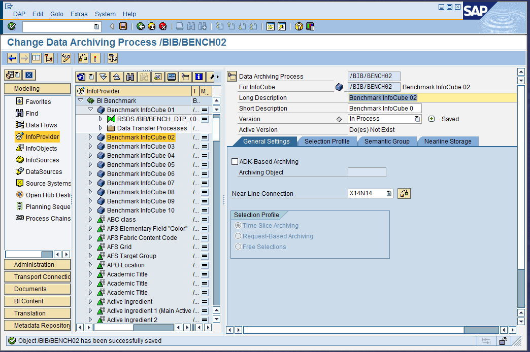
Figure 8-128 SAP Data Warehousing Workbench: Changing data archiving process
The Log Display window (Figure 8-129) opens. It indicates that all related tables have been created in the NLS database.

Figure 8-129 SAP Data Warehousing Workbench: Log Display
5. To check whether these newly created tables are column-organized, use the DBACOCKPIT (Figure 8-130).
a. From your SAP BW system, call transaction DBACOCKPIT.
b. Select your NLS system and then choose Space → Single Table Analysis in the navigation frame.
c. In the Table and Indexes Details area, enter the table name in the Name field and choose Enter. You can see if the table is column-organized in the Table Organization field on the System Catalog tab page.

Figure 8-130 SAP DBA Cockpit: Properties of a single table
6. Alternatively, you can check the newly created table using db2look. To run db2look, as instance owner, log on to the server that is hosting the NLS database and run the command as follows:
db2look -d <DBNAME> -a -e -t <TABLENAME>
Example 8-15 shows the DDL of OABENCH02-P table.
Example 8-15 The DDL for OABENCH02-P table generated by db2look
------------------------------------------------
-- DDL Statements for Table "X14N14 "."/B49/OABENCH02-P"
------------------------------------------------
CREATE TABLE "X14N14 "."/B49/OABENCH02-P" (
"PK_DBENCH02P" INTEGER NOT NULL ,
"CHNGID" VARCHAR(42 OCTETS) NOT NULL ,
"RECORDTP" VARCHAR(3 OCTETS) NOT NULL ,
"REQUID" VARCHAR(90 OCTETS) NOT NULL )
IN "X14#DB6#DIMD" INDEX IN "X14#DB6#DIMI"
ORGANIZE BY COLUMN;
-- DDL Statements for Primary Key on Table "X14N14 "."/B49/OABENCH02-P"
ALTER TABLE "X14N14 "."/B49/OABENCH02-P"
ADD CONSTRAINT "/B49/OABENCH02-P~0" PRIMARY KEY
("PK_DBENCH02P");
-- DDL Statements for Unique Constraints on Table "X14N14 "."/B49/OABENCH02-P"
ALTER TABLE "X14N14 "."/B49/OABENCH02-P"
ADD CONSTRAINT "/B49/OABENCH02-P~1" UNIQUE
("CHNGID",
"RECORDTP",
"REQUID");
After the NLS tables have been created, regardless whether they are row-organized or column-organized, the rest of the NLS operations are the same. For more information, see the SAP documentation Enabling SAP NetWeaver Business Warehouse Systems to Use IBM DB2 for Linux, UNIX, and Windows as Near-Line Storage (NLS)7:
Select <Your SAP NetWeaver Main Release> → Operations → Database-Specific Guides.
8.9.3 Configuration for BLU Acceleration on NLS
If you are using column-organized tables on the NLS database, you must increase the database configuration parameters SHEAPTHRES_SHR and SORTHEAP to meet the special memory requirements for column-organized tables. Also, INTRA_PARALLEL and MAX_QUERYDEGREE must be set to ANY. See SAP Note 1851832 for more information about SAP standard parameter settings.
8.9.4 NLS specific limitations
When you use column-organized tables for NLS InfoCubes and DataStore objects, the following restrictions might apply:
•Starting with DB2 Cancun Release 10.5.0.4, the conversion of existing row-organized NLS tables, using DB6CONV, to column-organized tables is supported. This does not apply on DB2 10.5 FP3aSAP or earlier fix packs.
•As of DB2 Cancun Release 10.5.0.4, adding columns is supported, if the corresponding NLS objects are created as column-organized tables. Other table layout changes are not directly supported in SAP NLS. If you are running on DB2 10.5 FP3aSAP or earlier, or you want to perform any other layout changes than adding columns in the SAP BW system, manual steps are required.
8.9.5 Benefits of BLU Acceleration for SAP NLS on DB2
SAP NLS on DB2 profits from BLU Acceleration in the same aspects as SAP BW does:
•Query performance is improved due to the column-oriented data store.
•Less tuning is necessary and no secondary indexes have to be maintained.
•The total storage consumption is reduced due to the advanced compression capabilities of DB2 with BLU Acceleration.
1 https://help.sap.com/saphelp_nw73/helpdata/en/d5/cd581d7ebe41e88cb6022202c956fb/content.htm?frameset=/en/32/5e81c7f25e44abb6053251c0c763f7/frameset.htm
3 See http://service.sap.com/notes (authentication required)
4 In newer service packs, the menu has been rearranged.
6 Anastassia Ailamaki, David J. DeWitt, Mark D. Hill, Marios Skounakis, Weaving Relations for Cache Performance, Morgan Kaufmann Publishers Inc., 2001, ISBN:1-55860-804-4
..................Content has been hidden....................
You can't read the all page of ebook, please click here login for view all page.