2
Verilog HDL, Communication, and Control
As C/C++ is a major language for programming vision algorithms, Verilog HDL/VHDL is a major language for designing analog/digital circuits. These two types of languages share common properties: a textual description consisting of expressions, statements, and control structures. One important difference is that HDLs explicitly include the notion of time and connectivity. As in other types of high-level programming languages, there are numerous design languages such as Impulse C, VHDL, Verilog, SystemC, and SystemVerilog, to name a few. In addition, Verilog HDL is one of the most widely used HDLs, along with VHDL, and its syntax is very similar to that of C, allowing vision engineers to be comfortable starting a circuit design.
This HDL was standardized in IEEE Standard 1364-2005 (IEEE 2005), resembles C, and covers a wide range constructs, from gate level to system level. SystemVerilog in IEEE Standard 1800-2012 (IEEE 2012) is a superset of Verilog-2005. In addition to the modules in Verilog-2005, SystemVerilog defines more design elements such as the program, interface, checker, package, primitive, and configuration. In addition, the language interface, VPI, in Verilog-2005 is generalized into DPI. This book is mostly based on Verilog-2005 (IEEE 2005).
This chapter introduces the Verilog syntax, the communication, and control modules. For the Verilog syntax, we will learn the minimal amount of syntax and grammar necessary for designing a vision architecture. (Refer to (Stackexchange 2014; Tala 2014) for introduction and questions.) The behavioral model, which is a high-level description similar to C, is adopted in various pieces of coding throughout this book. For the design method, we will learn the concept of communication, such as synchronous and asynchronous communication, and that of control, such as datapath method and distributed control.
2.1 The Verilog System
The overall structure of a design system consists of two modules: a test bench (TB) (a.k.a. test fixture) and unit under test (UUT) (a.k.a. device under test). The UUT is a target design that is to be implemented on hardware to execute a certain algorithm. The TB is not a part of the design, but a utility for testing the UUT (Figure 2.1). Aided by a simulator, the TB generates pattern vectors as inputs to the simulated UUT, gathers the output, and compares it with the expected values, generating a warning message or counting the errors, allowing any incorrect design to be accurately caught. After simulation and testing, the UUT is synthesized for devices such as FPGA, CPLD, and ASIC, aided by synthesis tools and libraries. While the two modules are programmed by the same HDL language, their properties differ greatly. The target module must consist of synthesizable Verilog codes only, but the test bench can consist of both synthesizable and unsynthesizable Verilog codes.
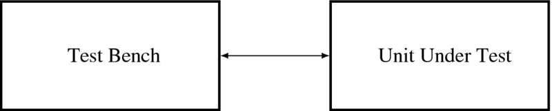
Figure 2.1 The Verilog system: TB-UUT modules
For a vision system, the UUT can be considered as hardware that executes a certain vision algorithm, receives a series of images, and emits the results through input and output ports. For proper testing, the TB must provide a set of representative image examples to detect any possible blind spots in the algorithm or design that were not noted at the programming stage. For example, if we are designing a stereo matching system, the TB must supply a pair of images to the UUT and assess the output from the UUT by comparing the results with the predicted disparities.
Because our concern is a vision system, in the next chapter we will develop a TB-UUT system, called a vision simulator, dedicated to vision.
2.2 Hello, World!
To become familiar with Verilog HDL, let us start by comparing it with C language. Simply put, the syntax of Verilog is very similar to that of the C programming language. The major features in common are the case sensitivity, control flow keywords, and operators. The major differences are the logic values, variable definition, data types, assignment, concurrency, procedural blocks with begin/end instead of curly braces, and compilation stages. While a C program must be compiled once, aided by a compiler, an HDL program may undergo two stages, RTL in the HDL and netlist in the synthesizer.
Because the level of language is high enough, many algorithms in vision can be written in Verilog HDL, if not for synthesis. For example, the ‘hello world’ examples for Verilog and C are listed side by side below.
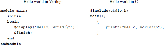
When executed using a Verilog simulator, the program outputs the same string as that of the C program. A program in Verilog always starts with module and ends with endmodule, after some possible headers. The scope is delimited by begin and end instead of the curly braces in C. In addition, there are many common features between the two languages. To make this program work, a file containing the above contents, hello.v, is provided and executed with a Verilog simulator to obtain the string, Hello, world! with a one-line feed. There are numerous simulators available, such as Verilog-XL, NCVerilog, VCS, Finism, Aldec, ModelSim, Icarus Verilog, and Verilator, to name a few. In addition, there are integrated development environments (IDEs) such as Altera Quartus and Xilinx ISE for editing, simulating, debugging, synthesis, testing, and programming.
When programming in Verilog HDL, there are three hardware description methods: structural description, behavioral description, and mixed description. A structural description is used to describe how the device is connected internally at the circuit and gate level. A behavioral description is used to describe how the device should operate in an imperative manner (cf. object-oriented and declarative in SystemVerilog). Considering the complexity of vision algorithms, we will follow the behavioral description method most of the time in this book.
As the next step, let us design a simple adder, a four-bit adder, using the behavioral model.
where a, b, and c are all four-bit integers. The source codes are included in the file, adder.v.
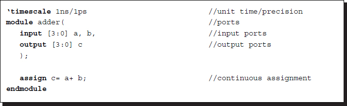
Listing 2.1 A 4-bit adder: adder.v
The module adder is the target design module, written in RTL syntax, to be simulated and possibly synthesized. It can be considered a procedure having two input arguments a and b and one output argument c, considered a call by value protocol (instead of call by reference). In the declaration section, three ports (similar to arguments in C) are declared as input and output. However, the argument directions are not formally specified in C. The statement assign c=a+b indicates that c is changed as soon as a or b is changed. This assignment, called a continuous assignment, is designed for the behavior of the combinational circuit.
In addition to the main modules, a TB must also be used to examine the adder module. The test bench, tb.v, is shown below.
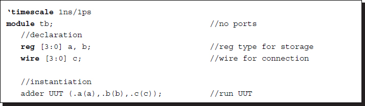
Listing 2.2 A test bench: tb.v
Because this module was designed only for testing, no port declaration is needed. It consists of two concurrent constructs: instantiation and an initial block, which may appear in arbitrary order. Instantiation is used to activate the adder module by calling the module as a statement. This module will be activated whenever the input values are changed. Unlike C, where all variables must be declared and defined before the statements referencing them, the input variables may not be defined lexically before instantiation but must be defined somewhere inside the same module. In the initial block, the values for the input ports are generated according to the designer's scheme. In a more elaborate system, the desired values must be generated according to the target algorithm, be compared to the actual values, and indicate the location of the errors.
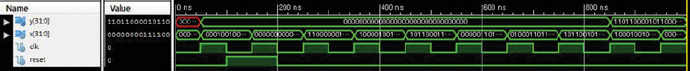
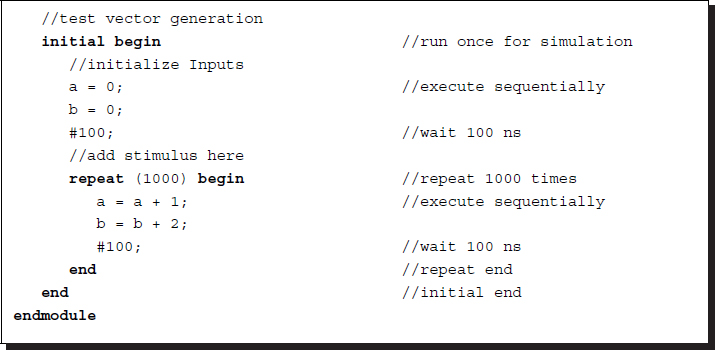
Figure 2.2 The simulator output: timing diagram
In a typical IDE system such as Altera Quatus (with ModelSim) and Xilinx ISE (ISIM or ModelSim), the Verilog simulator shows the values of the variables in a timing diagram (Figure 2.2). The left side of the figure shows the data and variables along with their values, in binary format. The horizontal axis is a time axis with the units specified in the target module. In this diagram, the variable values are shown in both numeric and signal forms. After a successful simulation, the system enters the synthesis stage during which a net-list file is generated, which can be observed in a schematic diagram.
2.3 Modules and Ports
An arbitrarily large system can be built by connecting small modules with input and output ports in a hierarchical manner. As such, a hierarchical hardware description structure is realized that allows the modules to be embedded within other modules. In C, this mechanism is realized through procedure calls with parameter passing, forming nested calls. In Verilog HDL, each module definition stands alone, and the modules are not nested. To connect the modules, higher-level modules create instances of lower-level modules and communicate with them through input, output, and bidirectional ports. In this sense, an instantiation is similar to a function call in C.
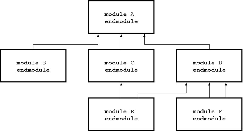
Figure 2.3 A hierarchy of modules
Figure 2.3 illustrates a system consisting of six modules in a hierarchical connection. In this system, the top module A calls (i.e. instantiates) B, C, and D; C calls E; and D calls E and F twice. An instantiation creates a circuit, and thus the code means that E and F are created twice, respectively.
To avoid a naming conflict, every identifier must have a unique hierarchical path name. The hierarchy of modules and the definition of items such as tasks and named blocks within the modules must have unique names. As with the connected modules, the hierarchy of names forms a tree structure, where each module instance, generated instance, task, function, named begin-end, or fork-join block defines a new hierarchical level or scope in a particular branch of the tree. The name of the module or module instance is sufficient to identify the module and its location in the hierarchy. Therefore, a module can reference a module below it (downward referencing), a module above it (upward referencing), and a variable (variable referencing).
Communication between modules is specified through ports, similar to arguments in C. However, there are significant differences between the two languages in terms of the nature of the arguments used. Unlike C, the direction of the ports must be specified using an input, output, or inout. In addition, the port types must be specified in terms of net-type and reg-type only, regardless of whether scalar or vector data are used. Typically, the input-output pair must be declared as reg-wire. The variable reg retains its value until it is changed by executing corresponding statements, and the variable wire simulates a passive wire whose value is determined by the driver, reg.
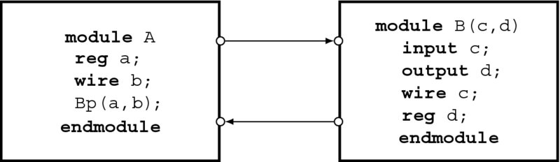
Figure 2.4 Connecting two modules by ports
Figure 2.4 illustrates this concept. Module A calls module B with two arguments, a and b. In this figure, the pair, a-c, is declared by reg-wire, and the pair, b-d, is declared by wire-reg. (In actuality, wire b and wire c are omitted.) This concept holds, in general, for a reg-net type pair, which simulates a driver-physical wire.
The net data types represent physical connections between structural entities such as gates. A net will not store a value (except for the trireg net), but its value will be determined by the values of its drivers. If no driver is connected to a net, its value has to have a high-impedance (z).
There are two ways to name the ports: positional (a.k.a. in-place) and named association, without allowing a mixed association. In the example, instantiation p(.d(b), .c(a)) in a named association is equivalent to instantiation p(a,b) in a positional association. The ports are either scalar or vector in reg-type and net-type but not in arrays or variables.
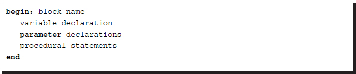
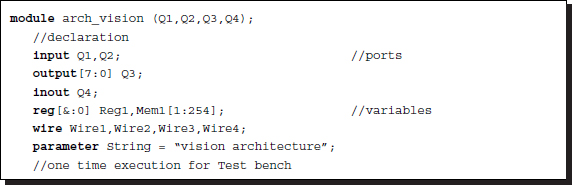
A module is the region enclosed between the keywords module and endmodule that contains all of the Verilog constructs except compiler directives having a certain structure.
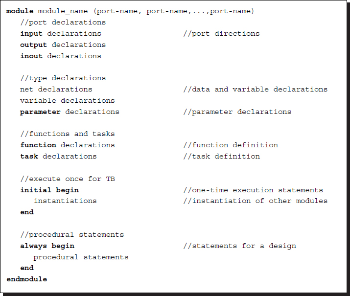
Listing 2.3 Module constructs
Followed by the keyword, module is the module identifier and port list. The main body of the module consists of a port declaration, variable declaration, function and task definition, and statements in the initial and procedural blocks, which are defined between begin and end. Among them, the initial block, which is executed once, is provided for a test bench. The order of all constructs, except the statements inside begin and end, does not matter.
The port list can be specified by the in-place or name list. The I/O declaration defines the direction of data flow for the ports. The variables are declared into three types: net type, variable type, and parameter. The function and task correspond to a function and procedure in C: a function returns a result, but a procedure does not. In addition, a procedure itself can be a statement, but a function cannot. The initial block is executed once and is therefore used for a design simulation. The module under test herein must put in the initial block. The main statements appearing in the procedure statements are specified by always.
2.4 UUT and TB
As previously mentioned, a design usually consists of a main module called the device under test (DUT) (or UUT), and another module called the test bench (TB) (or test fixture). A UUT is designed for synthesis, but a test bench is not. A test bench consists of test vectors (test suite or test harness), a UUT, and an instantiation. A set of test vectors must be generated and applied to an instantiated UUT as a stimulus so that the responses may be observed. Just like any other module description, a test bench is written in Verilog. A language-based test bench is portable and reproducible. The syntax of a TB is as follows.
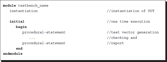
Listing 2.4 The test bench constructs
The structure consists of an instantiation and initial block. The purpose of an instantiation is to call the UUT, similar to a procedure call in C. However, unlike C, the argument values are defined later in the initial block. The purpose of an initial block is to provide argument values to the UUT and observe the output from the UUT and to provide other jobs such as comparing the output with the expected values, counting errors, and issuing warnings, all under the control of the designer.
A detailed description is shown in Figure 2.5. As shown on the left, the TB sends test signals to the DUT and receives the response in return. The internal structure of the TB is illustrated in detail on the right. A simulation with the TB is realized by an instantiation in the initial block. The pattern generator provides a set of test patterns including critical input cases that are supplied to both the DUT and the algorithm, which is to be executed by the UUT. Both responses from the TB and algorithm are collected, observed, and compared by the comparator to see if any mismatches exist. The observation results are reported outside by characters, diagrams, or graphs.
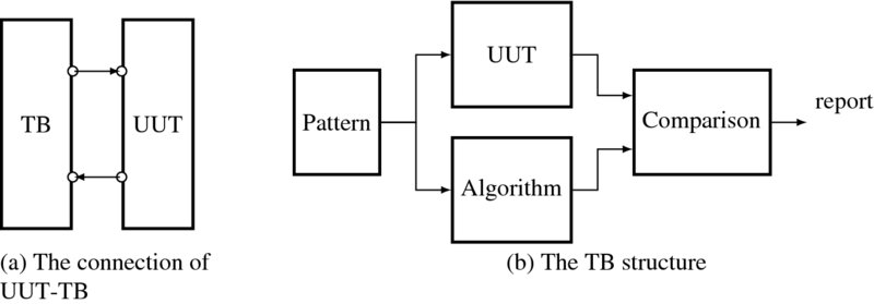
Figure 2.5 The UUT and the TB
2.5 Data Types and Operations
Thus far, we have learned the concepts of the UUT-TB and module-port. Now, let us describe in detail the syntax needed for constructing such modules. A value set is a set of data types designed to represent the data storage and transmission elements in a digital system. The Verilog value set consists of four basic values, 0 and 1, for ordinary logic, and x and z for unknown and high-impedance states. For example, one bit can have the values, 1'b0, 1'b1, 1'bx, and 1'bz, where the bases are 'b (binary),'o (octal), 'd (decimal), which is the default value, and 'h (hexadecimal).
There are three groups of data types: net data type, variable data type, and parameter. The net data type represents physical connections and thus does not store a value (except trireg). Its value is determined by the values of its drivers and thus has high impedance if disconnected. The exception is trireg, which holds the previously driven value even when disconnected from the driver. The driver connection is represented by a continuous assignment statement. The net type consists of wired logic (wire, wand, and wor), tri-state (tri, triand, trior, tri0, tri1, and trireg), and power (supply0 and supply1).
Among the net types, the wire and tri nets are used for nets that are driven by a single gate or continuous assignment. The wire net is used when a driver drives a net, and the tri net is used when multiple drivers drive a net. A wired net is used to model wired logic configurations. The wor/trior nets create a wired-or, such that if the value of any of the drivers is 1, the resulting value of the net is 1. Similarly, the wand/triand nets represent a wired-and, such that when the value of any driver is 0, the value of the net is 0.
The trireg net stores a value to model the charge storage nodes. It can be in one of two states: a driven state or a capacitive state, each of which corresponds to either a connected or disconnected state. The tri0 and tri1 nets represent nets with resistive pull-down and resistive pull-up devices on them. The supply0 and supply1 nets are used to model the power supplies in a circuit.
The variable type is an abstraction of a data storage element, as in C. The values are initially default and are determined later through procedural assignment statements. The variable data types are reg, integer, real, time, and realtime. The reg type is for a register that stores data temporarily in a procedural assignment. It is used to represent either a combinational circuit or a register that is sensitive to edges or levels of signals. The integer and time variable data types are not for hardware elements but for a convenient description of the operations. The integer and real types are general-purpose variables used for manipulating quantities that are not regarded as hardware registers. The time variable is used for storing and manipulating simulation-time values in cases where timing checks are required and for diagnostics and debugging purposes.
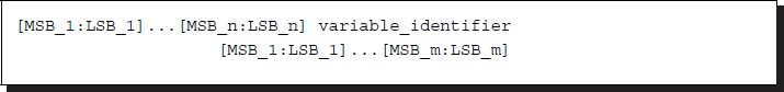
The net and variable types can be configured as arrays. An n-dimensional array is represented by a variable identifier and multiple indices: [MSB_1:LSB_1]...[MSB_n:LSB_n], where MSB and LSB are integers.
Listing 2.5 Arrays
The index convention is a row-major order, that is, the LSB changes most rapidly. A variable identifier is presented between the indices. The indices before and after the variable are called packed and unpacked, respectively. Packed arrays can have any number of dimensions. They provide a mechanism for subdividing a vector into subfields, which can be conveniently accessed as array elements. A packed array differs from an unpacked array, in that the whole array is treated as a single vector for arithmetic operations. An unpacked array differs from a packed array in that the whole array cannot be accessed, but rather each element has to be treated separately. (Unfortunately, the multidimensional packed array is possible only in SystemVerilog.) The memory is realized with a reg-type array.
Example 2.1 (Arrays) Examples of arrays are as follows.
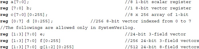
In the example, reg could have been replaced with any of the net or variable types.
Parameters do not belong to either a net or variable type but are constants. There are two types of parameters: module parameters (parameter, defparam) and specify parameters (specify, specparam). The parameters cannot be modified at runtime, but can be modified at compilation time to have values that are different from those specified in the declaration assignment, allowing a customization of the module instances. The non-local parameter values can be altered in two ways: the defparam statement, which allows assignment to parameters using their hierarchical names, and the module instance parameter value assignment, which allows values to be assigned in line during module instantiation.
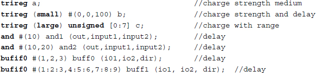
The net types are further specified by the drive strength and propagation delay. There are two types of strengths: charge strength for trireg and drive strength for net signals. The types of drive strength are supply, strong, pull, and weak. A signal with drive strength propagates from a gate output and a continuous assignment output. The charge strength specification is used with trireg with small, medium, and large. The net delay is specified with triple delays (rise, fall, transition), which indicate a rise delay, fall delay, and transition to a high-impedance value. Each of these delays can be further specified through (min:typ:max) keywords.
Example 2.2 (Strengths and delays) Some typical examples are as follows:
Now, let us consider the operators defined for the data types. Verilog defines a set of unary, binary, and ternary operators. For bit-wise logic, ∼, &, and | represent NOT, AND, and OR, respectively; ^ and ∼^/^∼ represent XOR and XNOR, respectively. The logical operators are !, &&, and || for NOT, AND, and OR, respectively. The reduction operators are unary operators, &, ∼&, |, ∼|, ^, and ∼^/^∼ representing AND, NAND, OR, NOR, XOR, and XNOR, respectively.
The arithmetic and shift operators are +, -, ∼, *, /, %, and ** for add, subtract, 2's complement, multiply, divide, modulus, and exponent, respectively. The relational operators are >, <, >=, and <=. In addition, the operators, == and =! are used for comparing two numbers excluding x and z. The operators, === and ==! are used for numbers with all four states considered.
The shift operators are >> and << for logical, and >>> and <<< for arithmetic shifts. The operators {,}, {{ }}, ?:, and , are concatenation, replication, conditional, and event-or, respectively.
Example 2.3 (Expressions) Some examples are as follows.
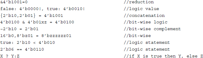
An event-or can be used instead of or in the following case: the expressions, @(clock or trig) regb = rega and @(clock,trig) regb = rega, are identical, indicating an assignment occurring when an event occurs on clock or trig. The delay expression is a triplet, (minimum:typical:maximum), as in (16'd10:16'd50:16'd100). The compiler directives are `include, `define, and parameter, where `define is used as a global, and parameter as a local to a module.
2.6 Assignments
Unlike in C, where only one type of assignment exists, there are two basic forms of assignments in Verilog: continuous assignment to drive the nets and procedural assignments to update the variables. Roughly speaking, they are introduced to specify explicitly whether an assignment is for combinational or sequential circuits.
The purpose of a continuous assignment is to represent a signal change in a combinational circuit by assigning values to the nets. The assignment operator is the pair assign and =. As in combinational logic, the left-hand side of this operator is changed whenever the value of the right-hand side changes.
Example 2.4 (Continuous assignments) The two expressions are effectively the same.
In the example, the two expressions are identical.
A delay, called a net delay, can be introduced by either a declaration or an assignment.
Example 2.5 (Delays) The continuous assignment with delay.
wire #100 a;
assign wire c = (#20) a + b;
In the first expression, any change of a will take effect after 100 unit times from the cause event. In a continuous assignment, changes in a or b will take effect with a change of c in 20 time units.
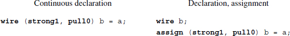
Similar to a delay, strength can be used as a declaration or an assignment. This applies only to assignments to scalar nets of the following types: wire, tri, trireg, wand, triand, tri0, wor, trior, and tri1. In other types, the strengths are fixed. For example, the strength value is always 1 for the following net types: supply1, strong1, pull1, weak1, and highz1. Similarly, the strength value for an assignment is always 0 for the following: supply0, strong0, pull0, weak0, and highz0.
Example 2.6 (Strengths) The strengths for a continuous assignment.

In the example, the first two expressions are identical: the order does not matter. The third expression is wrong: the strengths conflict with each other.
In the behavioral model, all of the statements are contained through the following procedures: initial construct, always construct, task, and function. The activity starts at the control constructs, initial and always. All of the initial and always constructs are enabled at the beginning of the simulation and run separately and concurrently. However, the initial construct is executed only once, but the always construct is permanently executed. There is no implied order of execution between the initial and always constructs. There is also no limit to the number of initial and always constructs that can be defined in a module.
An initial block is executed once and is externally concurrent. The assignments are either sequential (=) or concurrent (<=). This construct is not for a synthesis but for a simulation. Contrarily, an always block is executed permanently until $finish or $stop appears and is internally concurrent. The assignments are either sequential (=) or concurrent (<=). This construct is provided for synthesis.
The behavioral model is characterized by procedural assignments that are used to place values in variables. Unlike a continuous assignment, a procedural assignment does not have duration but holds a value until the next procedural assignment occurs for that variable. Procedural assignments appear within procedures such as always, initial, task, and function. These assignments can be thought of as triggered assignments that happen when the flow of execution in the simulation reaches an assignment within a procedure. Reaching the assignment can be controlled by event controls, delay controls, if statements, case statements, and looping statements.
There are three types of procedural assignments: = for blocking, <= for nonblocking, and assign-deassign and force-release for procedural continuous assignments. The first type of procedural assignment is blocking assignments that are executed before the execution of the statements that follow in a sequential block. The second type is nonblocking assignments, which are all concurrent, independent, and order-free within the same parallel block. All of the nonblocking assignments in a parallel block undergo a two-step execution: the first step (evaluation, execution, and scheduling) and an update.
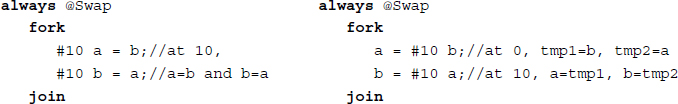
Example 2.7 (Blocking and nonblocking assignments) Swapping values.
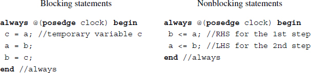
The swapping can be realized by both blocking and nonblocking assignments. With blocking assignments, a temporary variable is needed. With nonblocking assignments, two assignments are concurrent. The variables on the right-hand side are old values, and the ones on the left-hand side are new values obtained after the swapping.
The third type is a procedural continuous assignment with assign-deassign, which assigns values only when active and prevents ordinary procedural assignments from affecting the values of the assigned registers when inactive. This allows expressions to be driven continuously onto variables or nets. The assign part in a procedural continuous assignment statement overrides all procedural assignments to a variable. The deassign part in a procedural statement terminates a procedural continuous assignment to a variable. The value of the variable remains the same until the driver reg is assigned a new value through a procedural assignment or procedural continuous assignment. Yet another type is a procedural continuous assignment with force-release, which overrides a procedural assignment or procedural continuous assignment such that the variable resumes its original value when released.
Example 2.8 (assign-deassign) The procedural continuous assignment.
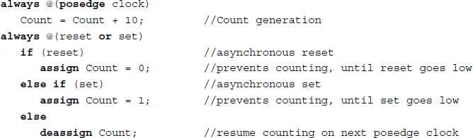
This is a counting example that contains a blocking procedural assignment and procedural continuous assignments. The counting event in the first always block is suppressed by the events in the second always block.
2.7 Structural-Behavioral Design Elements
Two design elements are possible: structural and behavioral. A structural design aims at a faithful hardware realization and uses fourteen gates such as and, or, not, nand, nor, xor, xnor, buf, buf0, buf1, notif0, and notif1 and twelve switches including cmos, nmos, rtran, and tran (see IEEE1364-2005 for a full list). In a structural model, an instance statement has the following form.

Listing 2.6 Instantiation
Here, the component name indicates the built-in gate.
Example 2.9 (Structure of module) An inhibition gate can be built as follows.

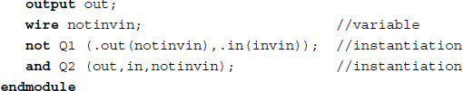
This example is for an inhibitor designed by two built-in gates. The arguments can be specified by either an in-place or a naming method.
As previously stated, all procedures in the behavioral model are defined in the following four statements: initial construct, always construct, task, and function. The initial and always constructs are enabled at the beginning of a simulation. The initial construct is executed only once, but the always construct is permanently executed. There is no implied order of execution between the initial and always constructs, and there is no limit to the number of initial and always constructs that can be defined in a module.
The behavioral (procedural) design is characterized by a procedural assignment for the blocking and nonblocking processing, a begin-end block for the scope, and a sensitivity list for the synchronization.

Listing 2.7 Procedural assignments
The statements with a blocking assignment are executed in order, but those with a nonblocking assignment are executed concurrently.
The scope is determined by the begin-end pair.
Listing 2.8 Scopes
A scope consists of declarations and procedural statements. The always block consists of a sensitivity list.

Listing 2.9 always block
Whenever any signal in the list is changed, the procedural statements in the scope are executed sequentially for blocking and concurrently for nonblocking.
The behavioral design is a high-level programming environment consisting of the following control flows: condition (if, case), loop (for, repeat, while, forever), and fork/join, which are all analogous to those in C.
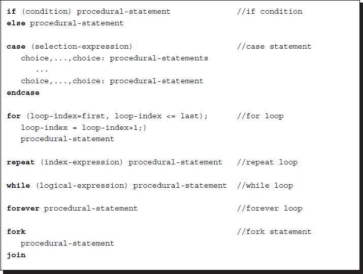
Listing 2.10 Conditionals
Here, a forever statement indicates an infinite loop. The fork/join pair is used for parallel processes. All statements (or blocks) between a fork/join pair begin their execution simultaneously upon the execution flow hitting the fork. The execution continues after the join upon completion of the longest-running statement or block between the fork and join.
Example 2.10 (fork/join) A simple example.
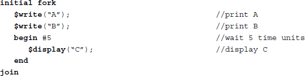
As a result of the simulation, we may have either sequence ‘ABC’ or ‘BAC’ printed out. In actuality, the order of simulations between the first and second writes depends on the simulator implementation.
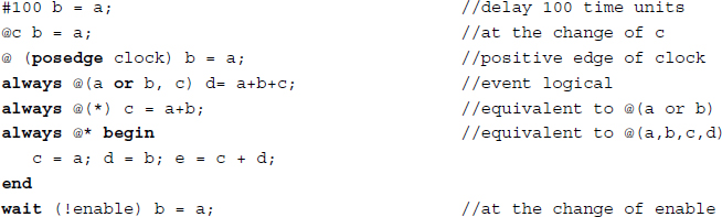
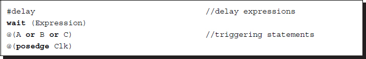
Procedure assignments have two methods for timing control: delay control and event control. Delay control is used to specify the time duration between when a statement is first reached and when the statement is actually executed. The event control expression allows a statement execution to be delayed until a simulation event occurs in a concurrently executing procedure. There are two types of simulation events: implicit and explicit. An implicit event indicates a change of value on a net or variable, and an explicit event indicates the occurrence of an explicitly named event triggered from other procedures.
The timing controls are realized through three methods: # for delay control, @ for event control, and wait for a combination of an event control and a loop. The event control can be made sensitive to signal edges with posedge and negedge.
Example 2.11 (Timing control) The timing control example.
The intra-assignment delay and event controls are the timing controls specified within an assignment statement. They delay the assignment of a new value to the left-hand side, but the right-hand side expressions are evaluated before the delay.
Example 2.12 (Intra-assignment) The example is as follows.
In the code on the left, both a and b are sampled and set at the same simulation time, resulting in a race condition. In the code on the right, the assignment is deferred 10 time units from the sampling.
Finally, a block of statements is a means for grouping two or more statements together so that they act syntactically as a single statement. There are two types of blocks: a sequential block with begin-end and a parallel block with fork-join.
2.8 Tasks and Functions
As in C, tasks and functions are common procedures that can be executed in different locations in a program. In addition, they are building-blocks of large procedures, and thus, the source descriptions can be easily built and debugged.
However, the two procedures have many different characteristics. Unlike those in C, a function must execute in one simulation time unit, but a task can execute in multiple time units, according to time-controlling statements. Another difference is that a function cannot enable a task, but a task can enable other tasks and functions. As for the arguments, a function has at least one input type argument and does not have an output or inout type argument, but a task can have zero or more arguments of any type. A function returns a single value, but a task does not return a value. A function has no output, but a task can have zero or more arguments of output and inout.
A function responds to an input value by returning a single value, but a task can return multiple values. Because of this response, a function is used as an operand in an expression, but a task is used as a statement.
A task is enabled from a statement that defines the argument values to be passed to the task and to the variables that receive the results. Control is passed back to the enabling process after the task has completed. If a task has timing controls inside it, then the time of enabling a task can be different from the time at which the control is returned. A task can enable other tasks, which in turn can enable still other tasks with no limit on the number of tasks enabled. Regardless of how many tasks have been enabled, control does not return until all enabled tasks have completed.
There are two forms for tasks: task name-endtask and task name-parenthesis-endtask.
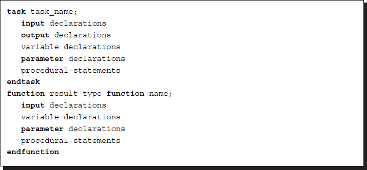
Listing 2.11 Tasks and functions
The standard formats of task and function are shown.
Tasks without and with the optional keyword automatic are called static tasks and automatic task, respectively. In a static task, all declared items are statically allocated and shared across all uses of the task executing concurrently. In an automatic task, all declared items are allocated dynamically for each invocation and cannot be accessed by hierarchical references. An automatic task can be invoked through the use of its hierarchical name.
Because a function is limited in a unit simulated time, it cannot contain any time-controlled statements with #, @, or wait and thus cannot enable tasks. A function definition contains at least one input argument but not output or inout. A function must include an assignment of the function result value to the internal variable that has the same name as the function name. Finally, a function should not have any nonblocking assignments.
To see the differences between tasks and functions, let us look at the factorial example, which is a typical example of recursion. The recursion can be realized by either a function or a task.
Example 2.13 (Factorial) The use of tasks and functions in factorial.
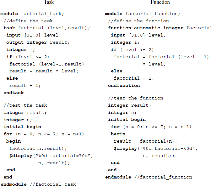
On the left, the task calls itself recursively, and on the right, the function is called iteratively. The factorial is a good example that shows the relationship between recursion and iteration.
2.9 Syntax Summary
The typical structure of a module is shown below, containing as many as possible Verilog constructs.
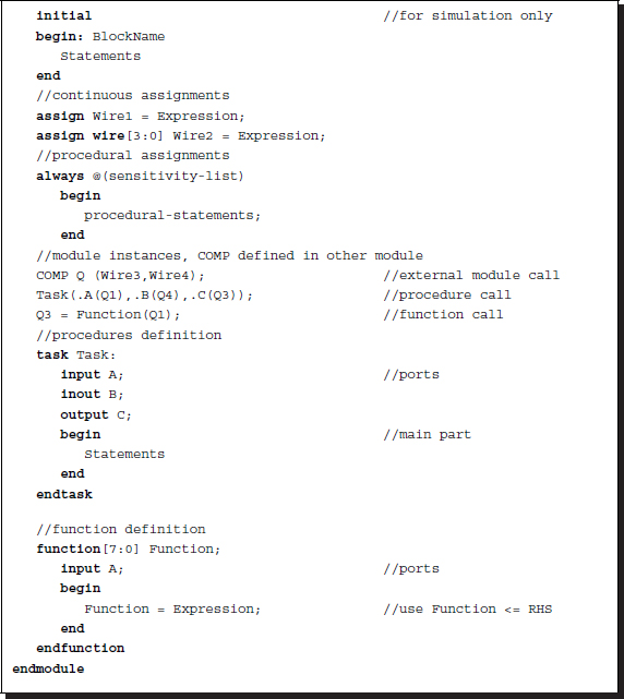
Listing 2.12 Summary of syntax
The module consists of declaration, initial block, procedural blocks, task, and function; the order may be arbitrary, and the execution is concurrent.
In addition, typical Verilog statements are listed below.
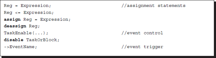
Listing 2.13 Summary of statements
The list contains continuous and procedural assignments, along with even triggers.
2.10 Simulation-Synthesis
Once the vision algorithm is written in the Verilog HDL complying with the Verilog syntax and grammar, the file with extension v must be compiled for simulation and then synthesis. In the simulation stage, the Verilog syntax is analyzed in the compilation stage, some design constructs such as generate are interpreted in the elaboration stage, and the compiled code written in Verilog grammar is executed in the simulation stage. The synthesis stage generates the standard design in the register-transfer level (RTL) and the target specific net-list, which needs to be downloaded into the devices such as field-programmable gate arrays (FPGAs), complex programmable logic devices (CPLDs), and application-specific integrated circuits (ASICs).
Because the synthesis is far more restricted than the simulation, we have to know the requirements for the constraints and use them in the design stage. There are three types of synthesis: logic gate synthesis, RTL synthesis, and behavioral synthesis. A logic gate synthesis is a synthesis from logic equations to logic gate diagrams; it is the simplest level of synthesis. In an RTL synthesis, all operations involve the transfer of data between registers using only a subset of the Verilog HDL. This is the state of the art of synthesis. A behavioral synthesis aims to convert a high-level description, like C, to desired circuits. Naturally, the HDLs have evolved toward this type of synthesis. For example, SystemVerilog is a superset of Verilog-2005 that has many high-level constructs, seemingly like C++. The behavioral design in Verilog-2005 HDL is a natural choice for vision algorithms, which involve complicated operations. In the future, SystemVerilog might play a significant role in designing vision algorithms, together with OpenCV.
Some of the guidelines in the synthesis stage are stated below. A combinational logic can be synthesized with continuous statements with assign and blocking statements with always. Continuous assignment can be used to represent simple circuits and must be used outside of always or initial blocks. Assign is used in top-level statements that are executed concurrently and continuously with all other top-level statements in the module. The left-hand side (LHS) of a continuous assignment statement must be a wire signal, whereas the variables on the right-hand side can be reg or wire signals.
The always blocks can represent complex combinational circuits; continuous assignment alone is not enough for complex combinational circuit. All circuit inputs must be included in the event control clause of the always block. No other signals must be included in the event control clause. No statements should be sensitive to rising or falling signal edges.
The sequential logic synthesis is designed by always blocks, in which statements execute concurrently and infinitely. Always blocks use an event control clause in order to prevent inefficient simulation behavior. The LHS of an assignment in an always block must be the type of reg. Within the same module, values must not be assigned to a single signal in two or more different always blocks. Use of both positive and negative edges of the same clock signal in an event control should be avoided. The common code template for Moore/Mealy-type finite state machines, available in mode Verilog platforms, may be useful.
Verilog consists of synthesizable and unsynthesizable Verilog code. For synthesis, the following must be considered. System functions and tasks are not for synthesis but for simulation and debugging. Verilog directives are not for synthesis. The initial block is not for synthesis. The values x and z are difficult to use in synthesis and should typically be avoided, unless there is a very specific reason to use them. Strength and delay statements cannot be synthesized. In conditional constructs (e.g., if, case), the default should be used, and don't-care values should be assigned to the output in order to simplify logic. Latches are inferred from incomplete if statements.
2.11 Verilog System Tasks and Functions
For simulation purposes, the Verilog HDL defines a set of system functions and tasks, analogously to those in C libraries. They are divided into ten categories: display tasks, file I/O tasks, timescale tasks, simulation control tasks, PLA modeling tasks, stochastic analysis tasks, simulation time functions, conversion functions, probabilistic distribution functions, command line input, and math functions. Knowing the system functions and tasks is essential to building a sophisticated system. Here, the format is the same as the normal tasks and functions.
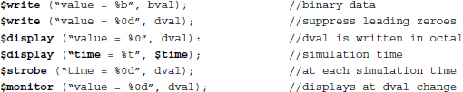
One of the most useful system functions might be the display tasks, called $display, $write, $strobe, and $monitor.

Listing 2.14 Display-write tasks
The display tasks may have a suffix such as b, o, d or h for binary, octal, decimal, and hex numbers, respectively; d is the default format for unspecified arguments. The basic display is write, and an advanced one is display, which adds a newline. In addition, strobe provides the ability to display simulation data at a selected time, and monitor provides the ability to monitor and display the values of any variables or expressions specified as arguments. The list of arguments includes strings, formats, and variables.
Example 2.14 (Display task) Examples of display tasks.
The system tasks and functions for file I/O are divided into the following four groups: open/close, file write, variable write, and read file. The file open and close tasks are $fopen and $fclose, respectively, which are very similar to those in C.
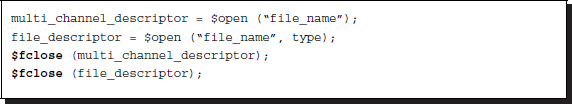
Listing 2.15 File open-close
The multichannel and file descriptors are 32-bit numbers. The argument type is a character string such as r for read, w for write, or a for append. A single bit in the multichannel descriptor represents the channel number and open/close. Thus, because multichannel descriptors are combined into one descriptor that contains all the open channel positions, multiple files can be written. A file descriptor is used to open a file according to type. The $fclose system task closes an open file.
The file output task names are $fdisplay, $fwrite, $fstrobe, and $fmonitor, defined similarly to the standard output, $display, $write, $strobe, and $monitor.
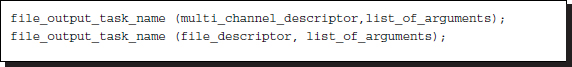
Listing 2.16 File output
]The first argument is either a multichannel descriptor or a file descriptor, which indicates where to direct the file output.
The system tasks, $swrite and $sformat, are used to write strings.
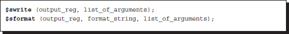
Listing 2.17 String output
The $swrite is the same as $fwrite except that the first argument is a reg. The $sformat is used for formatted writing. Files that are opened by file descriptors can be read only if they were opened with r type values.
Character or string is read by the following commands:
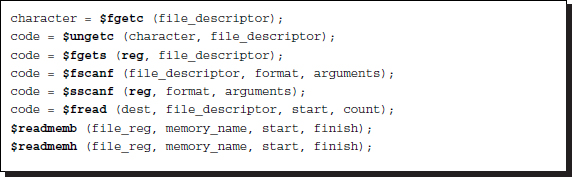
Listing 2.18 Character-string-text input
For the file and string input, system functions are provided for character ($fgetc, $ungetc), line ($fscanf, $sscanf), register ($fread), and text ($readmemb, $readmemh). $fgetc reads a character, and $ungetc returns the pointer to the previous position. $fgets reads a line until reg string is filled, a newline character is read and transferred to string, or an EOF condition is encountered. $fscanf and $sscanf are used for formatted reading from a file descriptor and reg string, respectively. $fread is used for reading binary data to fill the destination, which is reg or memory. The optional arguments start and count specify the starting point and the number of reading data, respectively. $readmemb and $readmemh read and load data from a test file to a memory. The text file may contain white spaces, comments, binary, or hexadecimal numbers. The start and finish addresses are optional. In addition, the addresses may be specified in the data file with the @ sign. The integer code represents an error condition.
For file access, the following commands are provided:

Listing 2.19 File positioning
The system function $ftell returns the offset between the beginning of the file and the file descriptor. $fseek is used to reposition the file to the position. $rewind is equivalent to $fseek(file_descriptor,0,0). $flush writes any buffered output to the opened files. During the file I/O system task and function, incidental errors might occur. $ferror is a system function that returns an error code. There are also command line inputs including the following: $test, $value, and $plusargs.
Example 2.15 (File I/O) The I/O examples are as follows.
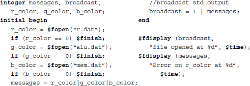
The simulation control tasks are $finish and $stop for exit and suspend, respectively. There are a set of system tasks and functions for queue and stack: $q_initialize, $q_add, $q_remove, $q_full, $q_exam.
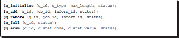
Listing 2.20 Queue
$q_initialize creates a queue (q_type=1) or stack (q_type=2) with the given queue id and maximum length. The push and pop operations are simulated with $q_add and $q_remove, respectively. The job_id is an integer input for identification. The inform_id is a user-defined integer. $q_full checks spaces in the queue, and $q_exam provides statistical information about queue activity. The status code is an integer that represents the error warning condition.
The simulation time can be observed by the following system functions: $time, $stime, and $realtime. There are system functions that convert numbers between different formats: $rtoi for real to integer, $itor for integer to real, $realtobits for real to binary, and $bitstoreal for binary to real. There are a set of random number generators: $random, $dist_uniform, $dist_normal, $dist_exponential, $dist_poisson, $dist_chi_square, $dist_t, and $dist_erlang.
There are integer and real math functions in Verilog system functions, which are identical to those in C. In addition to the Verilog system tasks/functions, there is a program interface with foreign functions written in C. With this interface, called VPI, the Verilog program can call user-defined functions and tasks and obtain the results. In image processing, the file transfer is the most essential operation between C programs and Verilog programs, which is not feasible in such operations.
2.12 Converting Vision Algorithms into Verilog HDL Codes
Computer-aided hardware design has evolved from the FSM, algorithmic state machine (ASM), HDL, and high-level synthesis (HLS). In the FSM method, the algorithm is represented by the state table and the state diagram. The design is in the logic equations and the minimization. In the FSM method with HDL, the representation is in the RTL (register transfer level) and the state diagram. The goal is to design the control logic from the state diagram and the datapath from the RTL. In ASM, the algorithm is represented by the RTL and the ASM chart. The control logic and the data path are designed by ASM chart and the RTL that are provided. The high-level synthesis works at a higher level of abstraction, starting with an algorithmic description in a high-level language such as SystemC, ANSI C/C++, OpenCL (Acceleware 2013), or HLS (Xilinx 2013). At the start, the designer develops the module functionality and the interconnect protocol manually. After that, the high-level synthesis tool constructs the architecture and transforms the functional codes into fully timed RTL codes. In the end, the RTL codes are used directly in a conventional logic synthesis flow to create a gate-level implementation.
One of the most fundamental abstractions is the control structure. The basic types of control structures are sequential, conditional, and loop. Most vision algorithms consist of mixtures of these control structures. Sequential computation means that statements are executed sequentially during each clock tick. Consider an algorithm consisting of N such statements. There are two ways to interpret the sequential computations in Verilog HDL (refer to the following codes).
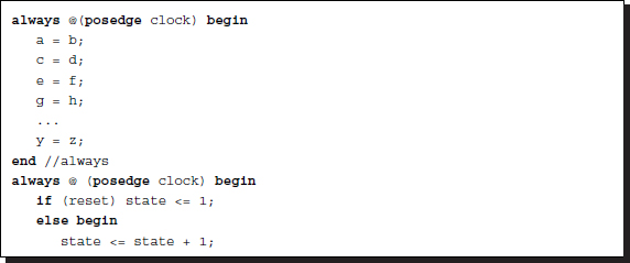
Listing 2.21 Sequential
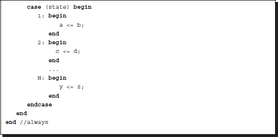
In the first code, the statements are executed sequentially by the blocking assignments. In the second code, the same is true for the sequential execution. However, there is a considerable difference between the two code segments. In the first code, the statements in a block are executed in one clock period, but in the second code, the statements are executed in each clock period. This mechanism is possible by the always-case combination. The sequential order is forced by the state and the statements are divided into blocks. Notice that the state increment and case block are concurrent.
In Verilog HDL, the available loop statements are for, while, repeat, and forever. The codes segments, with one exception, are listed side by side in the following. The one exception is forever, which represents permanent iteration. The assignments are all blocking, but they can also all be nonblocking, if necessary. For N statements, the loops need NT clocks for blocking and T clocks for nonblocking.
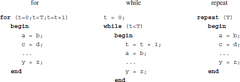
Regardless of the type of loop, all the statements in a block are executed in one clock period. Even for the blocking assignments, all of the statements in a block are executed in one clock time period. Actually, the loop is unfolded into a cascade of combinational modules, with each module executing each statement. (See unfolding (Wikipedia 2013b).)
In many cases, the statements must be separated and executed sequentially in a clock period, and repeated iteratively up to a predetermined number of times. Inserting delay statements between each blocking assignment is useless because the delay statements are not synthesized. It is possible to implement the sequential mechanism by combining case and if key words.
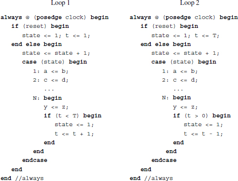
The code segments on the right also execute the statements iteratively up to the maximum number of iterations. (The statements can be either blocking or nonblocking, but not a mixture. Each statement can be replaced with a block of statements, which are either blocking or nonblocking.) In the Verilog loop statement, one iteration occurs in just one clock period. In this code, on the other hand, one iteration occurs in N clock periods.
There are many ways to code loops. First, the counter can be either auto-incrementing or auto-decrementing. The code segments above use both types of counters. There is another variation of the loop. The position of the if-statement can be either at the beginning or at the end of the statement block.
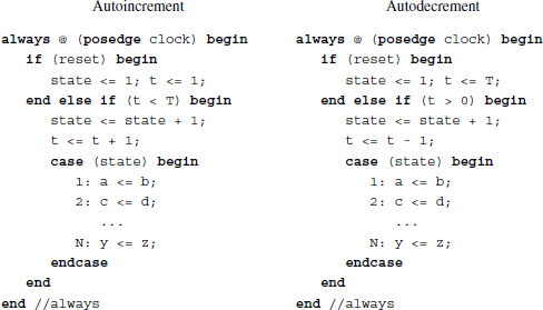
Unlike the previous code segments, the if-statement in this code is placed before the statement block. Like the previous code segments, two types of counters can be implemented. Therefore, there are four ways to configure the loops, depending on the if-statement positions and the counter types. If the assignment types are considered as well, then there are eight types of loops.
2.13 Design Method for Vision Architecture
Verilog HDL includes many design aids that transform the codes in high-level languages or diagrams to the codes in HDL. For example, the ‘C to HDL tools’ convert C program code into an HDL (or RTL) (Wikipedia 2013a). In the future, high-level languages might evolve to manage both software and hardware with the same unified compiler. Among others, the two packages, Altera OpenCL (Acceleware 2013) and Xilinx HLS (Xilinx 2013), are evolving rapidly. The design can be downloaded to the FPGAs (i.e. programming), converted to the hard copy of the ASIC chips (i.e. hard copy), or the full custom ASIC chips.
As an alternative, this book suggests a systematic method in designing a vision architecture. This method consists of three steps: 1) to prepare a vision algorithm, 2) to prepare a hardware algorithm, and 3) to code in Verilog HDL (see Figure 2.6). The first step is to provide a vision algorithm that consists of clear definitions of input and output, step-by-step procedures, (i.e. in time) for computing output, and all parameters and variables.
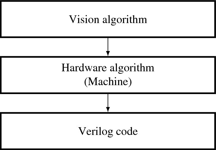
Figure 2.6 The three-step design method for vision architecture
The second step is to provide a hardware algorithm that represents a state machine. Consider that q(t) is the state, {x(t), y(t)} is an input-output pair, and T( · ) and H( · ) are the state transition function and the observation function, respectively. Then, a Moore machine is represented by the state equation:
This equation represents the general operations in vision algorithms, including sequential operation, parallel operation, iterative operation, neighborhood operation, recursive computation, and various memory structures.
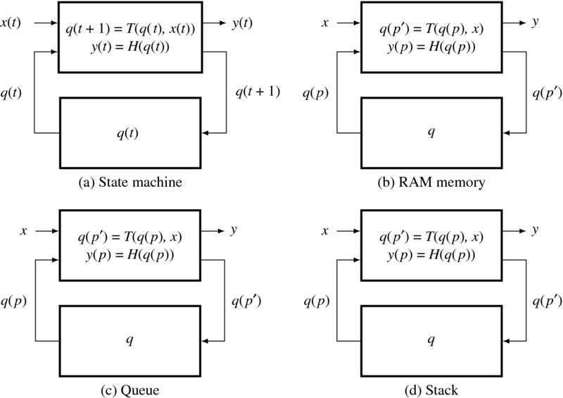
Figure 2.7 State machines for vision
A block diagram is shown in Figure 2.7(a). The state machine expresses how the state evolves and how the output is generated, as a function of time. To be a hardware algorithm, the standard representation, Equation (2.2), is not enough, because the use of resources (i.e. memory, ports, and connection) is not explicitly defined. A state equation must clearly specify which place of the memory must be read in order for the state to be updated, and which place of the memory must be replaced by the updated values. That is, the state equation must be rewritten in terms of the state memory and connectivity. To examine this further, we must specify the types of memories used most often in vision algorithms: RAM (random access memory), queue, and stack (Figures 2.7(b)–(d)). With RAM, an algorithm may access an arbitrary address in a memory for memory read and write. It may be a vector or a plane memory, often like an image plane. With a queue memory, an algorithm may push the data in one end and read data from another position of the queue. With a stack, an algorithm may read or write the memory by pop or push operations. A complicated system may consist of one or more such memories.
Let us denote the reading and writing positions of a memory by p and p′, respectively. Then the new state equation is
Here, the time index is omitted, because this equation is executed in every clock tick in a sequential circuit. Instead, an index, which represents the connectivity between memory and processor, is specified. The positions of a state memory, p for reading and p′ for writing, must be defined explicitly. Also, the assignment can be any of the Verilog assignments, continuous assignment (assign =), blocking (=) or nonblocking (i.e. <=). (The assignment, ←, collectively represents the three types of assignments.) In a neighborhood system, the access points must be a set of addresses within a neighborhood window. In most vision algorithms, the addresses are not random; they are fixed. Therefore, deriving addresses of the memory is one of the major tasks for specifying a hardware algorithm. To differentiate a hardware algorithm from a software algorithm, we use the term ‘(state) machine’ for hardware algorithm. Once the hardware algorithm is provided, we can express the architecture more easily by the Verilog HDL.
2.14 Communication by Name Reference
For vision processing, large amounts of data must sometimes be transferred between modules very rapidly. The data may be as small as a scalar or a vector or it may be as large as a set of image arrays or maps. The data width and data length are usually constant or known in advance. Verilog HDL allows only a scalar and a vector to be transferred between two ports. Therefore, the data must be a scalar, a byte, or a long vector constructed from a large array. The data must be transferred sequentially. There are basically two methods for building channels between modules: the reference-based method and the port-based method. In addition, there must one or more control programs that copy the original image and write the copy to the other module.
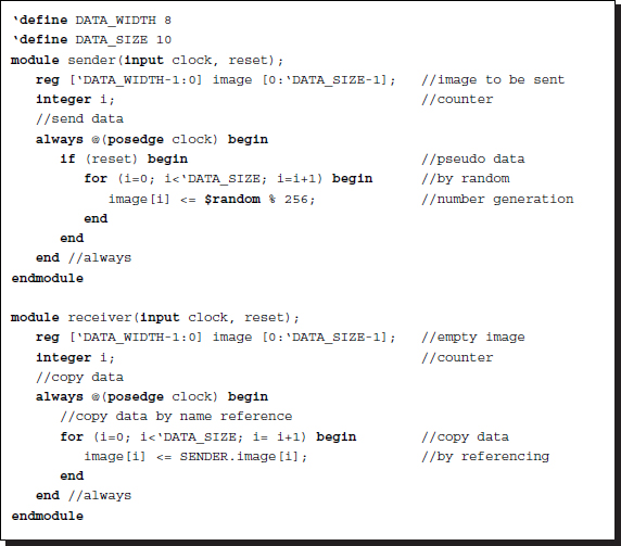
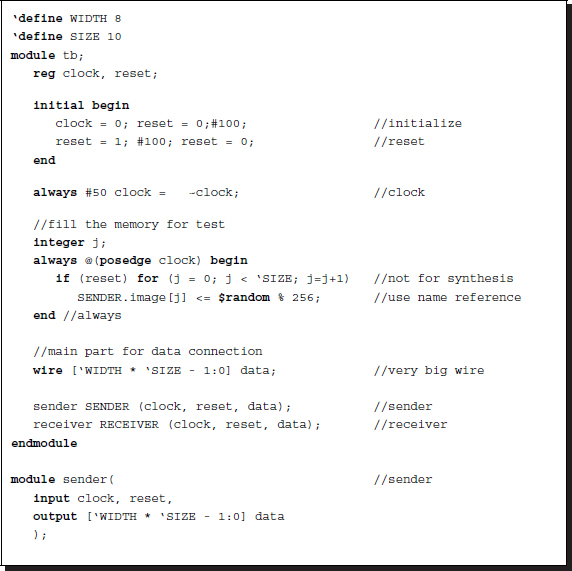
The reference-based method is useful when a large amount of image data must be transferred between modules, especially during simulations. Instead of using the physical ports, this method uses the name referencing in the hierarchical name referencing in Verilog HDL. Depending on where the control mechanism exists, there are three methods. Assume that a sender contains an image and a receiver wants copies of it, and that the two modules are instantiated as SENDER and RECEIVER in the third module. The first possibility is that the sender is active and the receiver is passive during the copying process.
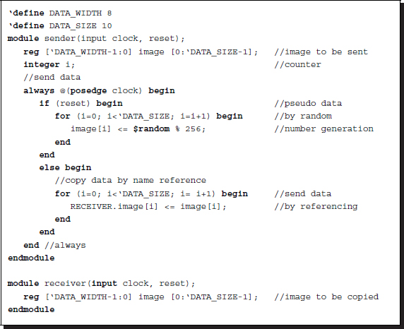
Listing 2.22 Referencing method: active sender and passive receiver
The image data is stored in the sender module and it is copied into the image in the other module. Without loss of generality, the image is filled by a random number generator for test purposes. In actual applications, the image must be an actual image or set of vectors or a scalar. (The same method is used repeatedly in the following for dealing with test images.) In the main part, an image element of the other module is referenced and copied using the image element in this module. Meanwhile, the receiver module contains an empty image. Because the receiver is passive, it does nothing, and the sender performs the copying process. No other module is necessary, though the sender and the receiver must be able to receive common signals: clock and reset signals.
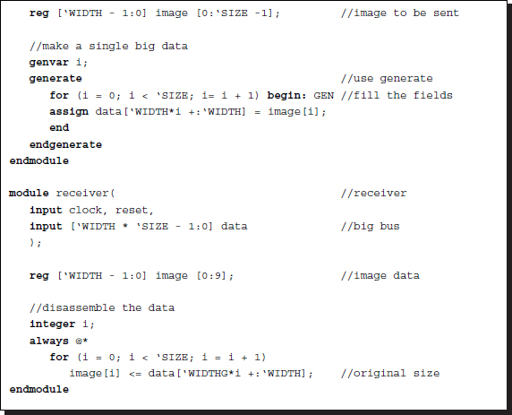
The second possibility is the opposite of the method above. In this case, the sender is passive and the receiver is active in the transfer control process.
Listing 2.23 Referencing method: passive sender and active receiver
In this case, the sender does nothing but prepare the image data. The receiver copies the image from the sender into its own image. The receiver references the image in the sender and copies its contents into the image.
The third possibility is the case where there is a third module that controls the copy process from the sender to the receiver. In this case, the sender and the receiver are both passive, and the third module is a controller for the communication process. The sender contains an image that is filled by a random number generator.
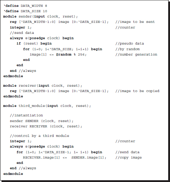
Listing 2.24 Referencing method: active third module
The receiver contains an empty image to be filled. In this case, the third module plays the role of transferring data between the sender and receiver. Any module can access the variables in the other modules by the hierarchical name referencing mechanism in Verilog HDL.
2.15 Synchronous Port Communication
Unlike in the simulation modules, the data in the synthesis modules must be transferred through ports. Because the port is one-dimensional, sending a multidimensional array through the port requires special care. On the sender side, the array must first be flattened into one-dimensional vectors and must be sent iteratively via the data stream. On the receiver side, the flattened vector must be popped out into the original array.
There are two methods that can be used to send a stream of data: synchronous and asynchronous data transfer. In synchronous transfer, the sender and the receiver start simultaneously. The role of the sender is to send the data units synchronously, one at a time, according to the clock. The role of the receiver is to receive the data synchronously, one at a time, from the common clock. There is no checking mechanism between the beginning and the end of the transfer, which is called a transaction, except by the common clock. The clock should allow for a slight delay between the times of sending and receiving.
For synchronous communications, there can be a third module that instantiates the sender and receiver and connects them by generating control signals.
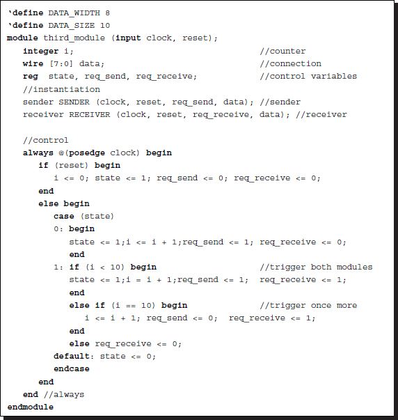
Listing 2.25 Synchronous communication: third module control
The third module must be careful to trigger the sender first during the request for the transaction and keep the receiver triggered at the end of the transaction. That is, the beginning and end of the transaction are delayed by one clock period between the sender and the receiver. Unlike the third module, the control program is the same in both the sender and the receiver.
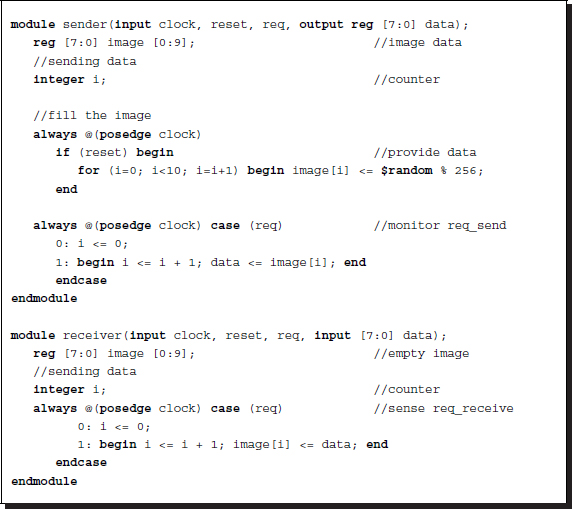
Another alternative is that the sender controls the data communication.
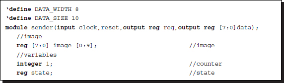
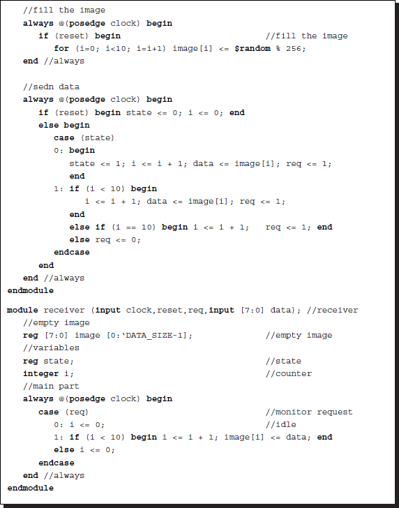
Listing 2.26 Sender active receiver passive
The sender controls the receiver by sending a request signal. Meanwhile, the receiver monitors for the request signal and continues to copy data as long as the request signal is asserted.
Note that the request signal is still active for one more clock period even after the counting ends. There is one clock period delay between the sender and the receiver.
2.16 Asynchronous Port Communication
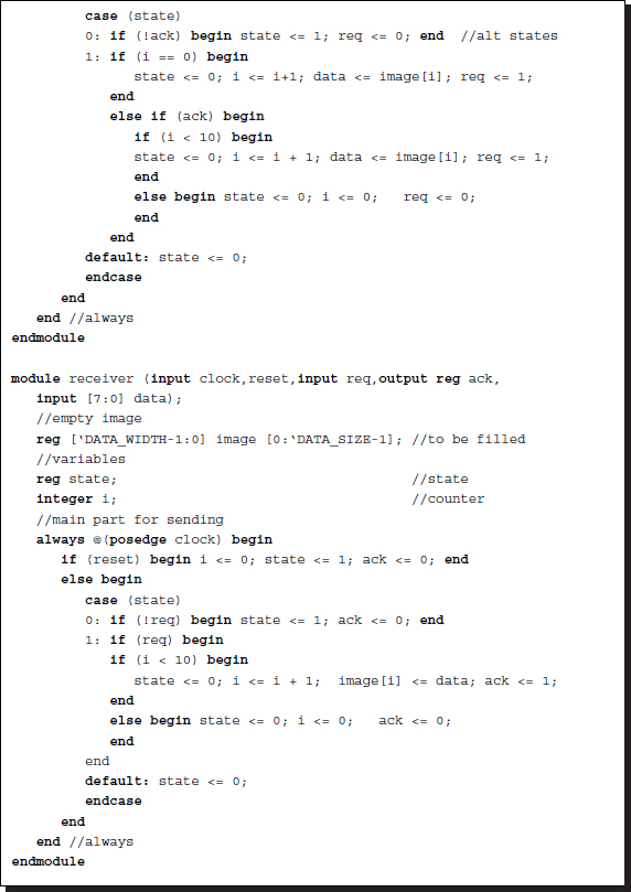
For secure communication, the transaction must include a two-phase or four-phase handshaking protocol. In both cases, when the two ports are linked, the data transfer is synchronized by a common clock. In the four-phase handshaking protocol, the quiet (i.e. idle) state is when neither the request nor the acknowledgement are zero. In the first step, the sender provides data and raises the request signal. In the second step, the receiver detects the rise in the request signal, receives the data, and raises the acknowledgement signal. In the third step, the sender detects the rise in the acknowledgement signal, lowers the request signal, and stops the data transfer. In the fourth step, the receiver detects the low request signal and lowers the acknowledgement signal. The four steps are repeated again as needed.
The two-phase handshaking protocol is a simplified version. There are two quiet states. The request and acknowledgement are both either zero or one. In the first step, the sender provides data and changes the request signal. In the second step, the receiver detects the change in the request signal, receives the data, and changes the acknowledgement signal. In the third step, the sender detects the change in the acknowledgement signal and the transaction ends. The loop is repeated forever.
The control mechanism on the sender's side is shown below. It consists of two states – one state for idling and the other state for sending data. The assumption is that the database to be sent is provided already before the transfer. This template shows that the database is a vector and that the transfer unit is a scalar in the vector. However, the database can be easily expanded to an image array. A counter is used to count the number of data units that are transferred.
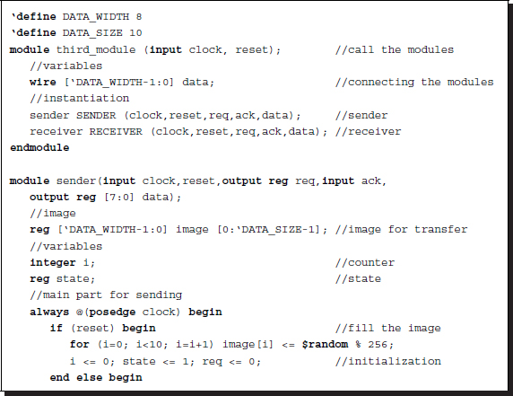
Listing 2.27 Handshaking
The sender provides the data to be sent and sends the request signal to the receiver. At each clock signal, the sender sends new data unit until the number of data units reaches a predefined number. Because the sender and the receiver know the number of data units, the acknowledgement signal is not necessary. On the receiver side, the control mechanism must be designed similar to the state machine. The receiver monitors for the request signal from the sender and begins to capture the data at each rising clock signal. When the number of data units that are captured reaches the predefined number, the receiver sends the acknowledgement signal to the sender.
The control mechanism must monitor the request bit from the sender and respond immediately when the request is asserted. At each clock signal, the data is captured and stored and the counter is incremented. The amount of received data is the same as that of the sent data. Upon completion, an acknowledgement signal is sent to the sender, which is not necessary in this simple case.
In this case, the handshaking protocol marks the beginning and end of the entire data transfer. During the transfer process, the data transfer and packet communication are synchronous. For secure communication, when the clock may be somewhat unreliable due to broadcasting, the handshaking protocols can be inserted between each data unit, resulting in asynchronous communication. There is a large difference between synchronous and asynchronous communications. For image transfer, a faster method is typically used, because the amount of data to be transferred is usually large.
Among the event-sensitive and level-sensitive control statements, the wait statement can be used for synchronizing or handshaking between the concurrent processes. (Unfortunately, it is not synthesizable in most systems.) It is sensitive to levels, as opposed to events, and is thus useful for handshake control (Lin 2008). In addition to the control mechanism, two semaphores (or messages) are needed, ‘send’ and ‘receive’ for example. The process waits until the expression of the semaphores is true, and then executes the statement. There are two types of handshake protocols: two-phase and four-phase. Further, each protocol has two alternative methods: sender-initiated and receiver-initiated (Lin 2008). The following is an example of a receiver-initiated code for the four-phase handshake protocol:
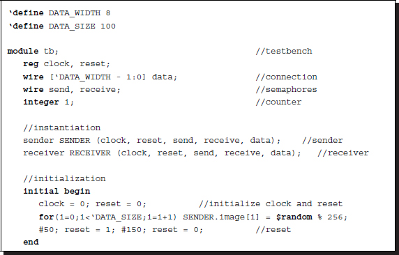
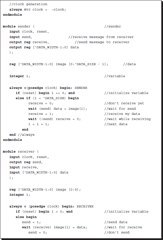
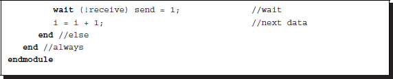
Listing 2.28 Port communication: Four phase handshake
Both modules run concurrently, and therefore, the messages are initialized (send = 1, receive = 0). Because it was initiated (send = 1), the sender provides data and sends a message (receive = 1). The receiver receives the data and acknowledges the successful transfer (send = 0). The sender then asks the receiver if it is ready to receive data whenever the sender is ready (receive = 0). This triggers the last wait statement in the receiver to change the state (send = 1). Finally, the two processes are back in their initial states waiting to repeat the above procedure.
The four-phase handshake is based on the semaphore levels, which results in four states, 0/0. 0/1, 1/0, and 1/1, for send/receive semaphore pairs. Conversely, the two-phase handshake can be designed by event-sensitive control. It has two states – 0/0 and 1/1 – for send/receive semaphores:

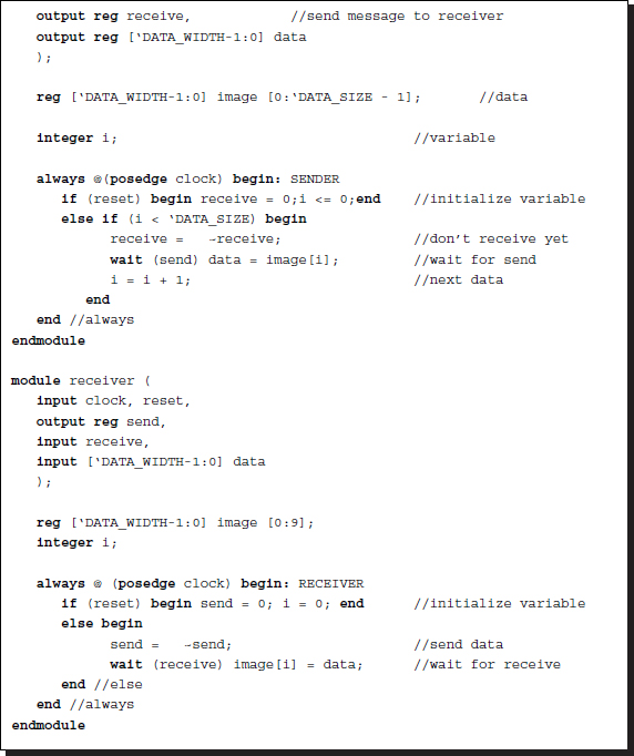
Listing 2.29 Port communication: two-phase handshake
Many problems exist in both the four-phase and two-phase (a.k.a. XOR) handshakes. In general, the two-phase handshake will have less overhead and better efficiency if a common clock drives the communicating modules. On the other hand, the four-phase handshake is more reliable and efficient when there is no such common clock.
Finally, the handshake and synchronous communication can be mixed, similar to packet communication, if the data size is very large. Between semaphore exchanges, a large amount of data can move between the sender and the receiver in an interval of many clocks.
2.17 Packing and Unpacking
For image processing, the transfer unit is usually a vector or a set of images or maps. The processor must access a pixel, a set of pixels for neighborhood operation, or the entire image for internal storage in an array. Regardless of the type of data, the transfer unit must be a vector, which is a simple byte for a pixel or a set of bytes for neighborhood pixels. Providing the input and output ports is not enough. The transfer mechanism introduced above must be embedded into both the sender and receiver ports.
For synthesis, the data communication must be based on the ports. If the size of the data to be transferred is identical to that of the port, the data can be transferred between the modules through the input and output ports. The port connections can be either scalar or vector, and no additional circuitry is needed if the port size is correct.
If the design resource allows for large ports, larger pieces of data can be transferred by assembling the sending data on the sender's side so that it fits the data bus and reassembling the data received at the receiver's side into data with the original size.
Listing 2.30 Communication: flattening the data
In this code, the generate block in the sender assembles a long data with the original data and the for block in the receiver disassembles the data back into the original data. This method involves the use of a very wide bus that fits the data. In actuality, there is a limit on the connection resource in a chip, which therefore limits the use of this method.
2.18 Module Control
A typical vision system may consist of one or more modules, thus requiring a control mechanism to execute the modules in systematic order: sequentially, concurrently, or partially in serial and partially concurrently. There are two basic control methods: centralized control and distributed control. In centralized control, a single control unit controls all the modules, whereas in distributed control, no separate control module exists, and therefore the modules control themselves interactively via some trigger (or strobe) signals.
The centralized control can be realized by decomposing the vision system into control unit and datapath (Hennessy and Parrerson 2012; Patterson and Hennessy 2012). In this control, the overall system consists of a controlling module and controlled modules, analogous to the control unit and datapath, respectively, in a typical computer. Between the control unit and the datapath, two types of signals are transferred: status and control signals. The control unit examines the status and determines the next order; the datapath operates according to the order and reports the status.
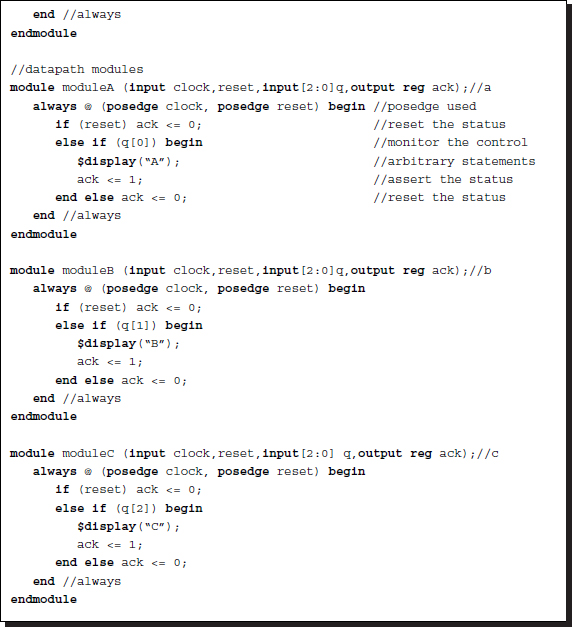
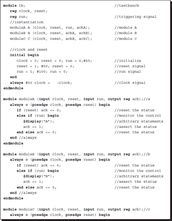
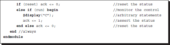
Let us consider how to control three modules, each printing A, B, C, respectively.
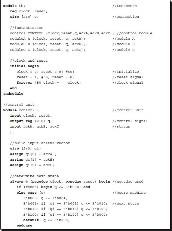
Listing 2.31 Control: FSM
The control unit consists of two parts: a status vector builder and an FSM. The status signals coming from each module are first assembled into an input vector via continuous assignment. The FSM then determines the next state depending on the present state and the input vector. The rule can be generally represented by case statements. (In this example, the rule is simple because the order of execution is sequential.) There is a delay in both the module response, from control output to status report, and the control unit response, from status input to control output. If we use negedge instead of posedge, the cycle time is only one clock instead of two clocks. (See the problems at the end of this chapter.)
The distributed control system needs trigger (strobe) signals to start the first module. Unlike handshaking, there are no feedback signals from the excited module to the exciting module. However, this mechanism can be realized via the event-sensitive and level-sensitive controls (@ and wait). The activated module may subsequently trigger other modules. This mechanism is repeated for all the modules, triggering the entire modules in a chain-reaction manner. Each module needs two trigger signals, one for triggering itself and another for triggering others at the end of the current process. The same problem can be coded in this method as follows:
Listing 2.32 Control: distributed
For this purpose, there must be a trigger signal supplied from the outside, which may be used to trigger the first module. There can be many variations of this method. Depending on the trigger signal, we may use either event-sensitive or level-sensitive control (@ and wait). The number of executions can be controlled by introducing the counters. This method is very efficient in its simplicity. However, if there are many modules, the complicated control needed cannot be easily designed. Furthermore, contentions may arise in the input trigger, because one or more modules might possibly try to control the same module. The other problem is the possibility of the occurrence of a loop, which cannot be easily detected in a system with many modules. This method is especially efficient when the number of modules is small and the control flow is sequential.
2.19 Procedural Block Control
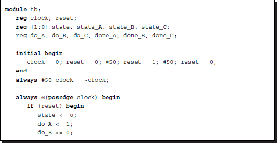
Inside the module, controlling of procedural blocks is an important issue in designing vision processors that must do reading, writing, and buffer updates, in addition to the main task of vision processing. The most fundamental approach is to use a large state machine that contains all the operations classified into states. Consider writing ABCABC..., using a three-state machine:
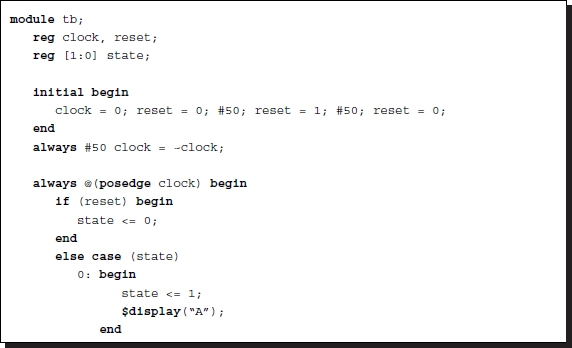
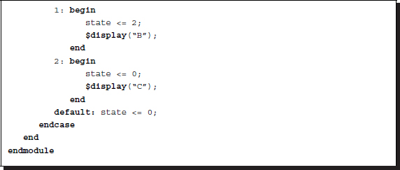
Listing 2.33 Controlling procedural block: state machine
The $display function must be replaced with appropriate vision operations. For a more sophisticated task, the state can be further divided into smaller states, in a hierarchical manner. The advantage of this method is the ability to use global variables, such as memory and array, which often contain huge amounts of image data. The disadvantage is that each state, which may be a large machine, cannot be simulated and synthesized separately.
The next approach is to divide the large state machine into separate procedural blocks, which are themselves state machines, even though the sizes are smaller.
Listing 2.34 Controlling procedural blocks: semaphores
Control of this system must be done by exchanging messages that they can use to control each other. In this case, situations in which a variable is driven by more than two procedural blocks have to be avoided.
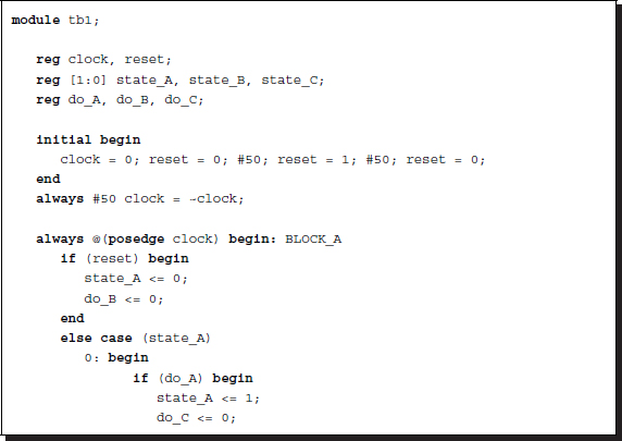
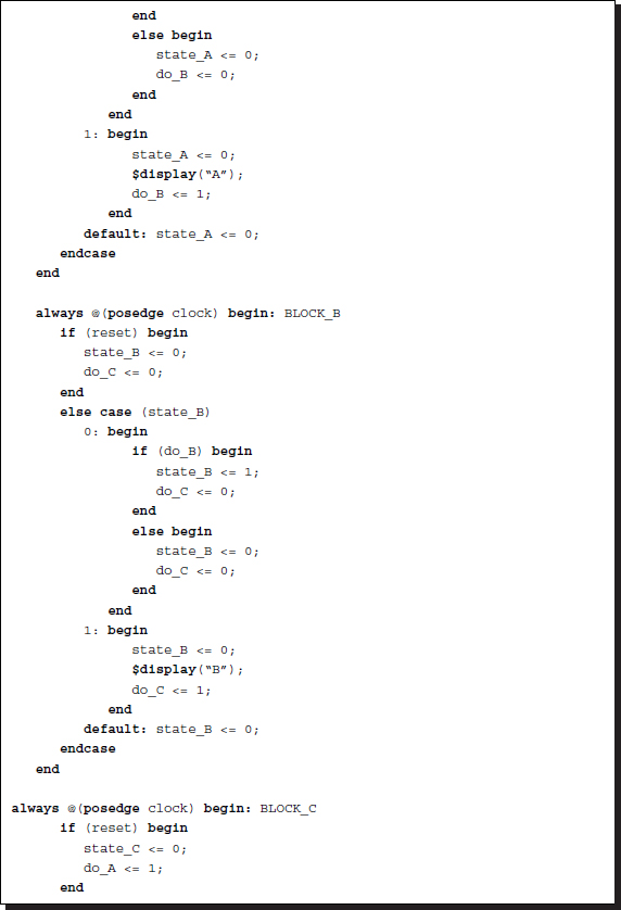
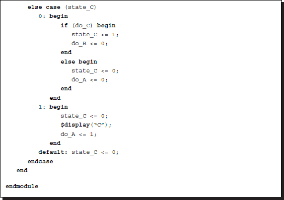
The other alternative is to use a control unit, which is a small state machine that receives states from the procedural blocks and sends control signals to them in return.
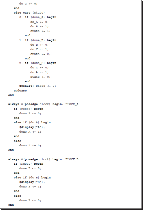
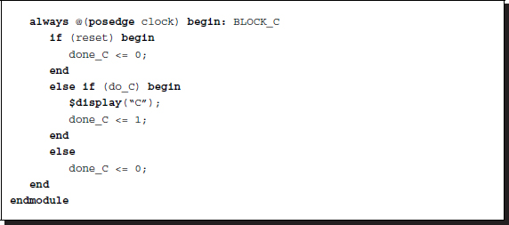
Listing 2.35 Controlling procedural blocks: control unit
This code actually generates AABBCCAA..., which can be corrected by counting the number of executions. This scheme is often called the datapath method, which consists of control unit and datapath. In the example, the states are done_A, done_B, and done_C. The control signals are do_A, do_B, and do_C.
Another method is to transfer the control in a daisy-chain manner, without relying on the control unit.
Listing 2.36 Control: internal trigger
The first module is initiated by the trigger signal coming from another module, except that the processes are initiated by the trigger signals from other processes executing in the same module. This computation has many variations: the shape of the trigger signal, the number of executions, the use of event-sensitive or level-sensitive control, or conditional statements.
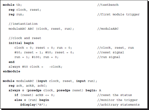
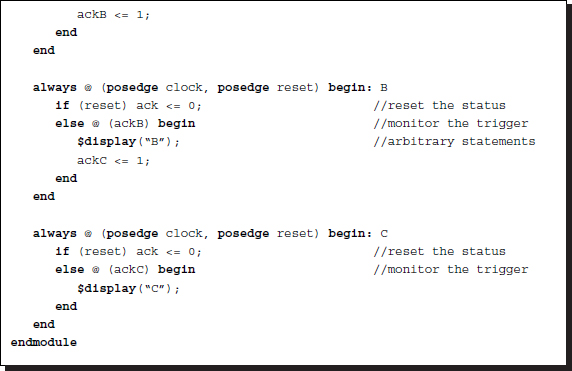
When the states or the procedural blocks are too large to be designed in the above manner, they must be designed with modules. In these large systems, the control structures must also be expanded to module control. The first alternative is the datapath method, in which a control unit receives states from each module, determines the next state, and then sends control signals to the modules. The second alternative is the use of semaphores, which are exchanged between modules, as a handshake, to control themselves.
The decision as to which entities, i.e. state, procedural block, or module, and which type of control, i.e. data path and handshake, to use depends on the nature and size of the vision problem.
Problems
- 2.1 [Handshake] Design two always blocks, where one block sends a sequence of random data to the other via a four-phase handshake. The transfer is synchronized to a common clock.
- 2.2 [Handshake] Design two always blocks, where one block sends a sequence of random data to the other via a two-phase handshake. The transfer is synchronized to a common clock.
- 2.3 [Handshake] Design two modules, where one module sends a sequence of random data to the other via a four-phase handshake. The transfer is synchronized to a common clock.
- 2.4 [Handshake] Design two modules, where one module sends a sequence of random data to the other via a two-phase handshake. The transfer is synchronized to a common clock.
- 2.5 [Packed and unpacked] Design a circuit that converts an unpacked array into a packed array.
- 2.6 [Packed and unpacked] Design a circuit that converts a packed array to an unpacked array.
- 2.7 [Control] In Listing 2.31, the negedge trigger is used in the control unit to prevent each state occupying two clock periods. What happens if, instead of negedge, posedge is used for the trigger?
- 2.8 [Control] Write a code that writes ABAB..., using two always blocks and semaphores do_A and do_B.
- 2.9 [Control] The following code contains a summation loop:
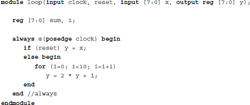
What happens in synthesis time in terms of the circuit structure?
- 2.10 [Control] Convert the previous code, so that the summation may be synchronized to the clock. Use the keyword if in front of the statement block.
References
- Acceleware 2013 OpenCL Altera http://www.acceleware.com/opencl-altera-fpgas (accessed May 3, 2013).
- Hennessy JL and Patterson DA 2012 Computer Architecture – A Quantitative Approach (fifth edn.). Morgan Kaufmann.
- IEEE 2005 IEEE Standard for Verilog Hardware Description Language. IEEE.
- IEEE 2012 IEEE Standard for SystemVerilog. IEEE.
- Lin MB 2008 Digital System Designs and Practices: Using Verilog HDL and FPGAs. John Wiley & Sons.
- Patterson DA and Hennessy JL 2012 Computer Organization and Design – The Hardware / Software Interface (Revised 4th Edition) The Morgan Kaufmann Series in Computer Architecture and Design. Academic Press.
- Stackexchange 2014 Verilog tag in stackoverflow http://stackoverflow.com/ (accessed Feb. 25, 2014).
- Tala DK 2014 Welcome to Verilog page http://www.asic-world.com/verilog/index.html (accessed Feb. 25, 2014).
- Wikipedia 2013a C to HDL http://en.wikipedia.org/wiki/C_to_HDL (accessed May 3, 2013).
- Wikipedia 2013b Unfolding (DSP implementation) http://en.wikipedia.org/wiki/Unfolding_(DSP implementation) (accessed May 16, 2013).
- Xilinx 2013 High level synthesis http://www.xilinx.com/training/dsp/high-level-synthesis-with-vivado-hls.htm (accessed May 3, 2013).