
4
Distribution Test-based Classifier
4.1 Introduction
When the observed signal is of sufficient length, the empirical distribution of the modulated signal becomes an interesting subject to study for modulation classification. In Chapter 2, the signal distributions in various channels are given. It is clear that the signal distributions are mostly determined by two factors, namely modulation symbol mapping and channel parameters. Assuming that the channel parameters are pre-estimated and available, the only variable in the signal distribution becomes the symbol mapping, which is directly associated with the modulation scheme. In Figure 4.1, signal cumulative distributions of 4-QAM, 16-QAM and 64-QAM are given in the same AWGN channel.
Figure 4.1 Cumulative distribution probability of 4-QAM, 16-QAM and 64-QAM modulation signals in AWGN channel.
By reconstructing the signal distribution using the empirical distribution, the observed signals can be analyzed through their signal distributions. If the theoretical distribution of different modulation candidates is available, there exists one which best matches the underlying distribution of the signal to be classified. The evaluation of equality between difference distributions is also known as goodness of fit (GoF), which indicates how the sampled data fit the reference distribution. Ultimately, the classification is completed by finding the hypothesized signal distribution that has the best goodness of fit.
There exist many different distribution tests which have been designed to evaluate the goodness of fit. Among them, we have selected three state-of-the-art distribution tests that have been adopted for modulation classification, and one customized distribution test created by the authors.
4.2 Kolmogorov–Smirnov Test Classifier
The Kolmogorov-Smirnov test (KS test) is a goodness-of-fit test which evaluates the equality of two probability distributions (Conover, 1980). The probability distributions can be either sampled empirical cumulative distribution functions (ECDF) or theoretical cumulative distribution functions (CDF). Massey first introduced the KS test (Massey, 1951) building on theories developed by Kolmogorov (1933) and Smirnov (1939). The KS test has since been applied in many signal processing problems.
Wang and Wang (2010) first adopted the KS test for modulation classification highlighting its low complexity against likelihood-based classifiers (Wei and Mendel, 2000) and high robustness versus cumulant-based classifiers (Swami and Sadler, 2000). Urriza et al. modified F. Wang and X. Wang’s method for improved computational efficiency (Urriza et al., 2011).
In this section, we first explain the basic theories of the KS test. The implementation of the KS test for modulation classification is presented subsequently.
4.2.1 The KS Test for Goodness of Fit
The KS test can be applied in two scenarios which are often referred to as the one-sample test and the two-sample test. In the one-sample test, a set of observed independent variables x1, x2, …, xn with an underlying cumulative distribution F1(x) and a hypothesized cumulative distribution function F0(x) is considered. The null hypothesis of the KS test is shown in equation (4.1),
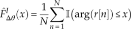
where F1(x) is replace by the empirical cumulative distribution function ![]() from the observed data, as defined in equation (4.2).
from the observed data, as defined in equation (4.2).
Given the definition of the goodness of fit, statistics is used to find the maximum difference between the underlying cumulative distribution function and the hypothesized cumulative distribution function, as shown in equation (4.3), where
the numerical calculation of the statistics is replaced by the maximum difference between the empirical cumulative distribution and the hypothesized cumulative distribution function, as given in equation (4.4).
According to the Glivenko–Cantelli lemma, the value of D is smaller if the null hypothesis is true, and the value is bigger if the underlying distribution and the hypothesized distribution are different (DeGroot and Schervish, 2010). Therefore, it is reasonable to reject the null hypothesis when the decision statistics ![]() is higher than a constant C [equation (4.5)].
is higher than a constant C [equation (4.5)].
The above distribution testing method is called the one-sample Kolmogorov–Smirnov test and the selection of the decision threshold constant is not presented as it is not needed in the application of modulation classification.
In the second scenario, there are two sets of observed independent variables x1, x2, …, xm and y1, y2, …, yn. Each of these data sets has an underlying distribution F(x) and G(x), respectively. To test if these two sets of data come from the same underlying cumulative distribution, the following Kolmogorov–Smirnov test null hypothesis ![]() 0 can be constructed [equation (4.6)].
0 can be constructed [equation (4.6)].
Following the same rule as in equation (4.1), the Kolmogorov–Smirnov test statistics in this scenario can be derived as the supremum of the distance between the two underlying cumulative distributions [equation (4.7)].
Practically, the underlying cumulative distribution function is replaced by the empirical cumulative distribution function sampled from the observations. The sampling of the empirical cumulative distribution function follows the same rule as in equation (4.2).
Equations (4.8) and (4.9) then lead to the updated test statistics representing the maximum distance between the empirical cumulative distribution functions from the two data sets [equation (4.10)].
The null hypothesis is then rejected if the test statistic ![]() is larger than a constant C, equation (4.11).
is larger than a constant C, equation (4.11).
The aforementioned method is named the two-sample Kolmogorov–Smirnov test. Both of the two applications of the Kolmogorov–Smirnov test can be used for modulation classification problems with different settings, and they achieve different performance characters. The implementation is presented in the following subsections.
4.2.2 One-sample KS Test Classifier
In the context of modulation classification, we assume there are a number N of received signal samples r[1], r[2],…,r[N] in the AWGN channel. The signal samples are first normalized to zero mean and unit power. The normalization is implemented on the in-phase and quadrature segments of the signal samples separately, as shown by
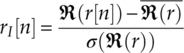
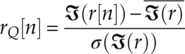
equations (4.12) and (4.13), where ![]() and
and ![]() are the mean of the real and imaginary part of the complex signal, with σ(ℜ(r)) and σ(ℑ(r)) being the standard deviation of the real and imaginary part of the complex signal. In the case of non-blind modulation classification, the effective channel gain and noise variance after normalization is assumed to be known. The assumption is demanding, while alternatives can be found where these parameters are estimated as part of a blind modulation classification. More discussion on blind modulation classification will be given in Chapter 7.
are the mean of the real and imaginary part of the complex signal, with σ(ℜ(r)) and σ(ℑ(r)) being the standard deviation of the real and imaginary part of the complex signal. In the case of non-blind modulation classification, the effective channel gain and noise variance after normalization is assumed to be known. The assumption is demanding, while alternatives can be found where these parameters are estimated as part of a blind modulation classification. More discussion on blind modulation classification will be given in Chapter 7.
For the hypothesis modulation ![]() ;(i) (with alphabet Am ∈ A, m = 1,…, M) in the AWGN channel with effective gain α and noise variance σ2, the hypothesis cumulative distribution function can be derived from the PDF of signal I-Q segments in equation (2.6), as given in equations (4.14) and (4.15).
;(i) (with alphabet Am ∈ A, m = 1,…, M) in the AWGN channel with effective gain α and noise variance σ2, the hypothesis cumulative distribution function can be derived from the PDF of signal I-Q segments in equation (2.6), as given in equations (4.14) and (4.15).
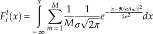
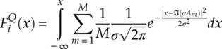
As only the cumulative distributions at the signal samples are need, the cumulative distribution values are calculated for ![]() and
and ![]() . These values are calculated during the classification process and therefore the computational complexity should be included as part of the classifier. The empirical cumulative distribution function is calculated following equation (4.2), as is shown in equations (4.16) and (4.17).
. These values are calculated during the classification process and therefore the computational complexity should be included as part of the classifier. The empirical cumulative distribution function is calculated following equation (4.2), as is shown in equations (4.16) and (4.17).
It is worth noting that the empirical cumulative distribution is independent of the test hypothesis. Therefore the collected values can be reused for all modulation hypotheses.
With both the hypothesized cumulative distribution function and empirical cumulative distribution function ready, the test statistics of the one-sample Kolmogorov–Smirnov test can be found for each signal I-Q segments, as set out in equations (4.18) and (4.19).
To accommodation the multiple test statistics calculated from multiple signal segments, they are simply averaged to create a single test statistics for the modulation decision making [equation (4.20)].

In some cases when the modulation candidates have identical distribution (e.g., M-PSK, M-QAM) on their in-phase and quadrature segments their empirical cumulative distribution can be combined to form an empirical cumulative distribution function with larger statistics [equation (4.21)].
Since the signal samples are complex, the multidimensional version of the KS test has been discussed in Peacock (1983) and Fasano and Franceschini (1987). We suggest that the corresponding test statistics can be modified to give equation (4.22),
where the test sampling locations are a collection of the in-phase and quadrature segments of the signal samples, as given in equation (4.23).
Regardless of the format of test statistics the classification decision is based on the comparison of the test statistics from all modulation hypotheses. The modulation decision is assigned to the hypothesis with the smallest test statistics [equation (4.24)].
4.2.3 Two-sample KS Test Classifier
When the channel is relatively complex and the hypothesis cumulative distribution function is difficult to be modelled accurately, the two sample Kolmogorov–Smirnov test may be much easier to implement. However, training/pilot samples are needed to construct the reference empirical cumulative distribution functions. Without any prior assumption on the channel state, K training samples x[1], x[2], …, x[K] are transmitted using modulation ![]() ;(i). The empirical cumulative distribution functions can be found following equations (4.16) and (4.17), and are given in equations (4.25) and (4.26).
;(i). The empirical cumulative distribution functions can be found following equations (4.16) and (4.17), and are given in equations (4.25) and (4.26).

The empirical cumulative distribution function of the N testing signal samples r[1], r[2],… r[N] are formulated in the same way as in equations (4.16) and (4.17). Using the two-sample test statistic in equations (4.10) and (4.19), the two-sample test statistics for modulation classification can be found as shown in equation (4.27).

In practical implementations, it is easier to quantize the testing range of x into a set of evenly distributed sampling locations.
The classification rule is the same as for the one-sample Kolmogorov–Smirnov test where the modulation hypothesis with the smallest test statistics is assigned as the classification decision.
4.2.4 Phase Difference Classifier
So far we have only used the signal in-phase and quadrature segments for the implementation of distribution test. However, there is an interesting signal feature that could be incorporated in the distribution test for exploiting the distinction of modulation signal in channels with phase or frequency offset. As discussed in Chapter 2, a fading channel, especially one with frequency offset, introduces severe distortion in the received signal in the form of a progressive rotational shift in its constellations. By measuring the phase difference between the adjacent signal samples, the phase difference error is reduced to a small constant. Thus, it has much less impact on the robustness of the modulation classifier.
In the AWGN channel where additive noises have Gaussian distribution, the theoretical CDF of the phase difference between adjacent signal sample vectors is derived by Pawula, Rice and Roberts (1982) as given in equation (4.28),
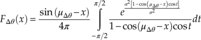
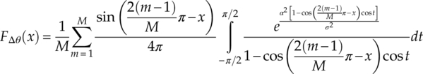
where μΔθ is the mean of the phase difference. The corresponding CDF for an M-ary PSK modulation can be found as shown in equation (4.29).
To implement the phase difference classifier, the only remaining task is to evaluate the empirical phase distribution by using equation (4.30).
Using the one-sample KS test, the test statistics of the phase difference test can be calculated by using equation (4.31).
The classification decision making is the same as the KS test in which the hypothesis with the smallest test statistics is selected as the classification decision.
4.3 Cramer–Von Mises Test Classifier
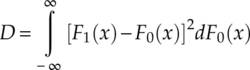
The Cramer–von Mises test (CvM test), also known as the Cramer–von Mises criterion, is an alternative to the KS test for goodness of fit evaluation (Honda, Oka and Ata, 2012). It is named after Harald Cramer and Richard Elder von Mises, who first introduced the method. Using the same one-sample test scenario as for the KS test, the test statistics is defined as the integral of the squared difference between the empirical CDF and the hypothesized CDF (Anderson, 1962), equation (4.33).
Anderson generalized the two-sample variety of the Cramer–von Mises test that evaluates the goodness of fit between two sets of observed data. The two-sample test statistics is given by equation (4.34),
where HM + N(x) is the empirical CDF of the combination of two sets of samples [equation (4.35)].
In practice the test statistic is evaluated in the form of summation instead [equation (4.36)].
Like the KS test classifier, the modulation classification decision using the Cramer–von Mises test is also assigned by the hypothesis with the smallest test statistics.
4.4 Anderson–Darling Test Classifier
Both the KS test and Cramer–von Mises tests are relatively less sensitive when the difference between distributions is at the tails of the distributions. This is because the cumulative distribution converges to zero and one at the tails of the distribution. To overcome this problem, Anderson and Darling proposed a weighted version of the Cramer–von Mises test called the Anderson–Darling (AD) test which gives more weight to tails of the distribution (Anderson and Darling, 1954). The test statistics is the Cramer–von Mises test with an added weight function w(x), equation (4.38).
The weight function is defined by equation (4.39),
which accentuates the distribution mismatch at the tails of the distribution when the CDF is close to zero or one. The classification is achieved by comparing the test statistics where the modulation candidate associated with the smallest test statistics is assigned as the modulation classification decision. The decision making is the same as in the KS test classifier and the Cramer–von Mises test classifier, equation (4.40).
4.5 Optimized Distribution Sampling Test Classifier
After the Kolmogorov–Smirnov test was proposed for modulation classification, Urriza et al. recognized the possibility to reduce its complexity further and potentially improve its classification performance (Urriza et al., 2011). The modification is enabled by establishing the sampling point prior to the distribution test using the theoretical cumulative distribution functions of modulation hypotheses. Assuming that there are two modulation candidates ![]() ;(i) and
;(i) and ![]() ;(j), the cumulative distribution functions of both modulations in a channel with known channel state information Fi(x) and Fj(x) are established prior to the distribution test. The sampling point lij in the test is found where the maximum distance between Fi(x) and Fj(x) is observed [equation (4.41)].
;(j), the cumulative distribution functions of both modulations in a channel with known channel state information Fi(x) and Fj(x) are established prior to the distribution test. The sampling point lij in the test is found where the maximum distance between Fi(x) and Fj(x) is observed [equation (4.41)].
The motivation for the optimized sampling location is first for the complexity reduction in calculating the empirical cumulative distribution function using the test data. Instead of calculating N values for the empirical cumulative distribution function using the optimized sampling location, the number is reduced to one. Additionally, assuming that the channel model is accurate, the optimized sampling location is a better utilization of the prior channel knowledge where the potential location for the maximum distance between the empirical cumulative distribution function and the theoretical cumulative distribution function is selected prior to the distribution test. It is especially effective when the number of samples available for constructing the empirical cumulative distribution function is limited and the ECDF may be misrepresenting the underlying CDF of the transmitted signal. In such cases, the maximum distance could occur where outliners are observed and the test results may be inaccurate for the classification decision making.
The test statistic is collected differently without the complexity of reconstructing the complete empirical cumulative distribution function and maximizing its difference with the hypothesized cumulative distribution. Instead the test statistic is only calculated by sampling the single location defined by equation (4.27), as shown in equation (4.42),
where ![]() is the empirical cumulative distribution probability at location lij, equation (4.43).
is the empirical cumulative distribution probability at location lij, equation (4.43).
The classification decision making is the same as in the Kolmogorov–Smirnov test classifier in the case of two-class classification.
Being an improvement of the Kolmogorov–Smirnov test classifier, the aforementioned modification was further improved and formalized by Zhu, Aslam and Nandi (2014). The rest of this section will be dedicated to their proposed version of the optimized distribution sampling test (ODST) classification.
4.5.1 Sampling Location Optimization
To further enhance the robustness of the Kolmogorov–Smirnov test-based classifier, Zhu et al. (2014) suggested using multiple pre-optimized sampling locations instead of a signal location suggested by Urriza et al. (2011). When using multiple sampling locations, there are two factors that need to be considered: the number of sampling locations and how they are found or optimized. Though using more sampling locations always provides more information when the distribution test is conducted, some locations may contribute much more than others. For example, two adjacent sampling locations would provide similar information of the ECDF/CDF, while having just one of them would be enough.
After analysis of the signal distribution and investigation of these distributions in various channel conditions, we have concluded that the local maximum of the difference between two CDFs is a good option. Here we define ![]() ij as a set of sampling locations with K individual sampling locations
ij as a set of sampling locations with K individual sampling locations ![]() . Following the rule for sampling location optimization, the sample locations should enable the distance between the CDFs Fi(x) and Fj(x) of modulation
. Following the rule for sampling location optimization, the sample locations should enable the distance between the CDFs Fi(x) and Fj(x) of modulation ![]() ;(i) and
;(i) and ![]() ;(j) to be a local maximum. A similar idea has been proposed by Wang and Chan (2012). The rule could then easily be converted to give the gradient of the function Fi(x) – Fj(x), which should be zero at the locations defined by
;(j) to be a local maximum. A similar idea has been proposed by Wang and Chan (2012). The rule could then easily be converted to give the gradient of the function Fi(x) – Fj(x), which should be zero at the locations defined by ![]() [equation (4.44)].
[equation (4.44)].
For the convenience of optimization of the sampling location using the theoretical distribution function, the CDFs in equation (4.28) can be replaced with their corresponding PDFs, resulting in the following updated rule given by equation (4.45).
It is worth noting that the sampling location is only optimized for the discrimination between modulation ![]() ;(i) and
;(i) and ![]() ;(j). If other modulation sets are considered, a different set of sampling locations should be optimized for the new modulation set.
;(j). If other modulation sets are considered, a different set of sampling locations should be optimized for the new modulation set.
4.5.2 Distribution Sampling
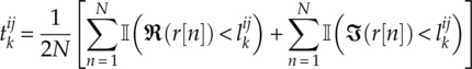
Having found the optimized sampling locations, the distributions are sampled to collect the necessary test statistics. Following the scenario in the previous section, we assume there is a piece of signal r[1], r[2],…, r[N] with N samples. The test statistics ![]() are sampled empirical cumulative distribution functions at the optimized sampling locations [equation (4.46)].
are sampled empirical cumulative distribution functions at the optimized sampling locations [equation (4.46)].
It is worth noting that these sampled values have also been suggested as distribution features by Zhu, Nandi and Aslam (2013).
Before classification decision making can proceed, the reference CDF for each hypothesized models has to be calculated as well. Among the two candidate modulations, the reference CDF values need to be sampled separately from each of them. For modulation ![]() ;(i), the reference CDF values
;(i), the reference CDF values ![]() are calculated using their theoretical CDF and the optimized sampling locations [equation (4.47)].
are calculated using their theoretical CDF and the optimized sampling locations [equation (4.47)].
The reference CDF values for modulation ![]() ;(j) are denoted with a slight difference. The order of i and j in the superscript is inverted so that the letter in front could represent where the reference value is gathered from. The actual computation follows the same method with only the CDF values being replaced by the those from modulation
;(j) are denoted with a slight difference. The order of i and j in the superscript is inverted so that the letter in front could represent where the reference value is gathered from. The actual computation follows the same method with only the CDF values being replaced by the those from modulation ![]() ;(j) [equation (4.48)].
;(j) [equation (4.48)].
4.5.3 Classification Decision Metrics
Having calculated the sampled CDF values and the reference CDF values from modulation hypotheses, the next step would be to evaluate the GoF between observed signals and hypothesized models. Unlike the KS test and other aforementioned distribution test classifiers, there are multiple sampling locations in this method. Therefore, the test statistics need be formulated as a combination of the sampled and reference CDF values. Before we present the test statistics formula, we first introduce the difference statistics that marks the difference between sampled values and reference values at individual sampling locations. The different statistics for hypothesized modulation ![]() ;(i) at the kth sampling location is defined as the difference between the sampled CDF at kth sampling location and the reference CDF value of modulation
;(i) at the kth sampling location is defined as the difference between the sampled CDF at kth sampling location and the reference CDF value of modulation ![]() ;(i) at the same sampling location [equation (4.49)].
;(i) at the same sampling location [equation (4.49)].
The corresponding expression for the alternative hypothesis of modulation ![]() ;(j) is given by equation (4.50).
;(j) is given by equation (4.50).
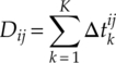
The above calculation results in k difference statistics for each modulation hypothesis. To combine these difference statistics into a signal test statistics, we have proposed two approaches. First, the test statistics Dij for hypothesized modulation ![]() ;(i) is formulated as a non-negative uniform linear combination of the difference statistics, as shown in equation (4.51).
;(i) is formulated as a non-negative uniform linear combination of the difference statistics, as shown in equation (4.51).
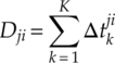
The corresponding expression for the alternative hypothesized modulation ![]() ;(j) is given by equation (4.52).
;(j) is given by equation (4.52).
Second, the test statistics Dij for hypothesized modulation ![]() ;(i) is formulated as a non-negative weighted linear combination of the difference statistics [equation (4.53)],
;(i) is formulated as a non-negative weighted linear combination of the difference statistics [equation (4.53)],
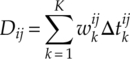
where ![]() is the weight for the difference statistics
is the weight for the difference statistics ![]() . The corresponding expression for the alternative hypothesized modulation
. The corresponding expression for the alternative hypothesized modulation ![]() ;(j) is given by equation (4.54).
;(j) is given by equation (4.54).

There are different ways of optimizing the weights. Among which, Zhu et al. used a genetic algorithm to train the weights with training signals (Zhu, Aslam and Nandi, 2014).
4.5.4 Modulation Classification Decision Making
The decision making in the optimized distribution sample test is different from that in the other distribution test-based classifiers. As the distribution sampling location is optimized between two modulation candidates, it could be easily implemented for a two-class classification problem. The decision is given by the modulation hypothesis which returns the smallest tests statistics [equations (4.55)].
If multi-class classification is required, the distribution test needs to be performed for every pair of two candidate modulations. The modulation candidate assigned the most time among all the paired distribution tests will be returned as the final classification decision.
4.6 Conclusion
In this chapter we have listed some of the distribution test-based classifiers. The distribution test-based classifiers are selected mostly for their computational complexity and suboptimal performance. Given that the channel parameters are known to the classifier, a one-sample KS test classifier or a two-sample KS test classifier achieves modulation classification by comparing the empirical distribution of the observed signal and the theoretical distribution of each modulation hypothesis. The Cramer–von Mises test classifier provides a better evaluation of the mismatch between the empirical distribution and hypothesis distribution, while the Anderson–Darling test classifier suggests a weighted evaluation of the goodness of it over the entirety of the signal distribution. The optimized distribution sample test is presented as an improved version of the KS test classifier with enhanced classification accuracy and robustness.
References
- Anderson, T. (1962) On the distribution of the two-sample Cramer–von Mises criterion. The Annals of Mathematical Statistics, 33 (3), 1148–1159.
- Anderson, T.W. and Darling, D.A. (1954) A test of goodness of fit. Journal of the American Statistical Association, 49 (268), 765–769.
- Conover, W. (1980) Practical Nonparametric Statistics, John Wiley & Sons, Inc., New York, NY.
- DeGroot, M.H. and Schervish, M.J. (2010) Probability and Statistics, 4th edn, Pearson, Boston, MA.
- Fasano, G. and Franceschini, A. (1987) A multidimensional version of the Kolmogorov-Smirnov test. Monthly Notices of the Royal Astronomical Society, 225, 155–170.
- Honda, C., Oka, I. and Ata, S. (2012) Signal Detection and Modulation Classification Using a Goodness of Fit Test. International Symposium on Information Theory and its Applications, Honolulu, HI, 28–31 October 2012, pp. 180–183.
- Kolmogorov, A.N. (1933) Sulla Determinazione Empirica di una Legge di Distribuzione. Giornale dell’ Istituto Italiano degli Attuari, 4, 83–91.
- Massey, F. (1951) The Kolmogorov-Smirnov test for goodness of fit. Journal of the American Statistical Association, 46 (253), 68–78.
- Pawula, R.F., Rice, S.O. and Roberts, J.H. (1982) Distribution of the phase angle between two vectors perturbed by gaussian noise. IEEE Transactions on Communications, 30 (8), 1828–1841.
- Peacock, J.A. (1983) Two-dimensional goodness-of-fit testing astronomy. Monthly Notices of the Royal Astronomical Society, 202, 615–627.
- Smirnov, H. (1939) Sur les Ecarts de la Courbe de Distribution Empirique. Recueil Mathematique (Matematiceskii Sbornik), 6, 3–26.
- Swami, A. and Sadler, B.M. (2000) Hierarchical digital modulation classification using cumulants. IEEE Transactions on Communications, 48 (3), 416–429.
- Urriza, P., Rebeiz, E., Pawełczak, P. and Čabrić, D. (2011) Computationally efficient modulation level classification based on probability distribution distance functions. IEEE Communications Letters, 15 (5), 476–478.
- Wang, F. and Chan, C. (2012) Variational-Distance-Based Modulation Classifier. IEEE International Conference on Communications (ICC), Ottawa, ON, 10–15 June 2012, pp. 5635–5639.
- Wang, F. and Wang, X. (2010) Fast and robust modulation classification via Kolmogorov-Smirnov test. IEEE Transactions on Communications, 58 (8), 2324–2332.
- Wei, W. and Mendel, J.M. (2000) Maximum-likelihood classification for digital amplitude-phase modulations. IEEE Transactions on Communications, 48 (2), 189–193.
- Zhu, Z., Aslam, M.W. and Nandi, A.K. (2014) Genetic algorithm optimized distribution sampling test for M-QAM modulation classification. Signal Processing, 94, 264–277.
- Zhu, Z., Nandi, A.K. and Aslam, M.W. (2013) Robustness Enhancement of Distribution Based Binary Discriminative Features for Modulation Classification. IEEE International Workshop on Machine Learning for Signal Processing, Southampton, 22–25 September, 2013, pp. 1–6.