
Routers as Distributed Systems
Come now and let us reason together.
— ISAIAH 1:18, THE BIBLE
Distributed systems are clearly evil things. They are subject to a lack of synchrony, a lack of assurance, and a lack of trust. Thus in a distributed system the time to receive messages can vary widely; messages can be lost and servers can crash; and when a message does arrive it could even contain a virus. In Lamport’s well-known words a distributed system is “one in which the failure of a computer you didn’t even know existed can render your own computer unusable.”
Of course, the main reason to use a distributed system is that people are distributed. It would perhaps be unreasonable to pack every computer on the Internet into an efficiency apartment in upper Manhattan. But a router? Behind the gleaming metallic cage and the flashing lights, surely there lies an orderly world of synchrony, assurance, and trust.
On the contrary, this chapter argues that as routers (recall routers includes general interconnect devices such as switches and gateways as well) get faster, the delay between router components increases in importance when compared to message transmission times. The delay across links connecting router components can also vary significantly. Finally, availability requirements make it infeasible to deal with component failures by crashing the entire router. With the exception of trust — trust arguably exists between router components — a router is a distributed system. Thus within a router it makes sense to use techniques developed to design reliable distributed systems.
To support this thesis, this chapter considers three sample phenomena that commonly occur within most high-performance interconnect devices — flow control, striping, and asynchronous data structure updates. In each case, the desire for performance leads to intuitively plausible schemes. However, the combination of failure and asynchrony can lead to subtle interactions.
Thus a second thesis of this chapter is that the use of distributed algorithms within routers requires careful analysis to ensure reliable operation. While this is trite advice for protocol designers (who ignore it anyway), it may be slightly more novel in the context of a router’s internal microcosm.
The chapter is organized as follows. Section 15.1 motivates the need for flow control on long chip-to-chip links and describes solutions that are simpler than, say, TCP’s window flow control. Section 15.2 motivates the need for internal striping across links and fabrics to gain throughput and presents solutions that restore packet ordering after striping. Section 15.3 details the difficulties of performing asynchronous updates on data structures that run concurrently with search operations.
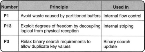
The techniques described in this chapter (and the corresponding principles invoked) are summarized in Figure 15.1.
In all three examples in this chapter, the focus is not merely on performance, but on the use of design and reasoning techniques from distributed algorithms to produce solutions that gain performance without sacrificing reliability. The techniques used to gain reliability include periodic synchronization of key invariants and centralizing asynchronous computation to avoid race conditions. Counterexamples are also given to show how easily the desire to gain performance can lead, without care, to obscure failure modes that are hard to debug.
The sample of internal distributed algorithms presented in this chapter is necessarily incomplete. An important omission is the use of failure detectors to detect and swap out failed boards, switching fabrics, and power supplies.
15.1 INTERNAL FLOW CONTROL
As said in Chapter 13, packaging technology and switch size are forcing switches to expand beyond single racks. These multichassis systems interconnect various components with serial links that span relatively large distances of 5–20 m. At the speed of light, a 20-m link contributes a round-trip link delay of 60 nsec. On the other hand, at OC-768 speeds, a 40-byte minimum-size packet takes 8 nsec to transmit. Thus, eight packets can be simultaneously in transit on such a link.
Worse, link signals propagate slower than the speed of light; also, there are other delays, such as serialization delay, that make the number of cells that can be in flight on a single link even larger. This is quite similar to a stream of packets in flight on a transatlantic link. A single router is now a miniature Internet.
TCP (Transmission Control Protocol) and other transport protocols already solve the problem of flow control. If the receiver has finite buffers, sender flow control ensures that any packet sent by the sender has a buffer available when it arrives at the receiver. Chip-to-chip links also require flow control. It is considered bad form to drop packets or cells (we will use cells in what follows) within a router for reasons other than output-link congestion.
It is possible to reuse directly the TCP flow control mechanisms between chips. But TCP is complex to implement. Disentangling mechanisms, TCP is complex because it does error control and flow control, both using sequence numbers. However, within a chip-to-chip link, errors on the link are rare enough for recovery to be relegated to the original source computer. Thus, it is possible to apply fairly recent work on flow control [OSV94, KCB94] that is not intertwined with error control.
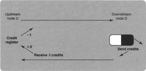
Figure 15.2 depicts a simple credit flow control mechanism [OSV94] for a chip-to-chip link within a router. The sender keeps a credit register that is initialized to the number of buffers allocated at the receiver. The sender sends cells only when the credit register is positive and decrements the credit register after a cell is sent. At the receiving chip, whenever a cell is removed from the buffer, the receiver sends a credit to the sender. Finally, when a credit message arrives, the sender increments the credit register.
15.1.1 Improving Performance
In Figure 15.2, if the number of buffers allocated is greater than the product of the line speed and the round-trip delay (called the pipe size), then transfers can run at the full link speed.
One problem in real routers is that there are often several different traffic classes that share the link. One way to accommodate all classes is to strictly partition destination buffers among classes. This can be wasteful because it requires allocating the pipe size (say, 10 cell buffers) to each class. For a large number of classes, the number of cell buffers will grow alarmingly, potentially pushing the amount of on-chip SRAM required beyond feasible limits. Recall that field programmable gate arrays (FPGAs) especially have smaller on-chip SRAM limits.
But allocating the full pipe size to all classes at the same time is obvious waste (P1) because if every class were to send cells at the same time, each by itself would get only a fraction of the link throughput. Thus it makes sense to share buffers. The simplest approach to buffer sharing is to divide the buffer space physically into a common pool together with a private pool for each class.
A naive method to do so would mark data cells and credits as belonging to either the common or the private pools to prevent interference between classes. The naive scheme also requires additional complexity to guarantee that a class does not exceed, say, a pipe size worth of buffers.
An elegant way to achieve the allow buffer sharing without marking cells is described in Ozveren et al. [OSV94]. Conceptually, the entire buffer space at the receiver is partitioned so that each class has a private pool of Min buffers; in addition there is a common pool of size (B – N * Min) buffers, where N is the number of classes and B is the total buffer space. Let Max denote the pipe size.
The protocol runs in two modes: congested and uncongested. When congested, each class is restricted to Min outstanding cells; when uncongested, each class is allowed the presumably larger amount of Max outstanding cells. All cell buffers at the downstream node are anonymous; any buffer can be assigned to the incoming cells of any class. However, by carefully restricting transitions between the two modes, we can allow buffer sharing while preventing deadlock and cell loss.
To enforce the separation between private pools without marking cells, the sender keeps track of the total number of outstanding cells S, which is the number of cells sent minus the number of credits received. Each class i also keeps track of a corresponding counter, Si, which is the number of cells outstanding for class i. When S < N · Min (i.e., the private pools are in no danger of depletion), then the protocol is said to be uncongested and every class i can send as long as Si ≤ Max.
However, when S ≥ N · Min, the link is said to be congested and each class is restricted to a smaller limit by ensuring that Si ≤ Min. Intuitively, this buffer-sharing protocol performs as follows. During light load, when there are only a few classes active, each active class gets Max buffers and goes as fast as it possibly can. Finally, during a continuous period of heavy loading when all classes are active, each class is still guaranteed Min buffers.
Hysteresis can be added to prevent oscillation between the two modes. It is also possible to extend the idea of buffer sharing for credit-based flow control to rate sharing for rate-based flow control using, say, leaky buckets (Chapter 14).
15.1.2 Rescuing Reliability
The protocol sketched in the last subsection uses limited receiver SRAM buffers very efficiently but is not robust to failures. Before understanding how to make the more elaborate flow control protocol robust against failures, it is wiser to start with the simpler credit protocol portrayed in Figure 15.2.
Intuitively, the protocol in Figure 15.2 is like transferring money between two banks: The “banks” are the sender and the receiver, and both credits and cells count as “money.” It is easy to see that in the absence of errors the total “money” in the system is conserved. More formally, let CR be the credit register, M the number of cells in transit from sender to receiver, C the number of credits in transit in the other direction, and Q the number of cell buffers that are occupied at the receiver.
Then it is easy to see that (assuming proper initialization and that no cells or credits are lost on the link), the protocol maintains the following property at any instant: CR + M + Q + C = B, where B is the total buffer space at the receiver. The relation is called an invariant because it holds at all times when the protocol works correctly. It is the job of protocol initialization to establish the invariant and the job of fault tolerance mechanisms to maintain the invariant.
If this invariant is maintained at all times, then the system will never drop cells, because the number of cells in transit plus the number of stored cells is never more than the number of buffers allocated.
There are two potential problems with a simple hop-by-hop flow control scheme. First, if initialization is not done correctly, then the sender can have too many credits, which can lead to cell’s being dropped. Second, credits or cells for a class can be lost due to link errors. Even chip-to-chip links are not immune from infrequent bit errors; at high link speeds, such errors can occur several times an hour. This second problem can lead to slowdown or deadlock.
Many implementors can be incorrectly persuaded that these problems can be fixed by simple mechanisms. One immediate response is to argue that these cases won’t happen or will happen rarely. Second, one can attempt to fix the second problem by using a timer to detect possible deadlock. Unfortunately, it is difficult to distinguish deadlock from the receiver’s removing cells very slowly. Worse, the entire link can slow down to a crawl, causing router performance to fall; the result will be hard to debug.
The problems can probably be cured by a router reset, but this is a Draconian solution. Instead, consider the following resynchronization scheme. For clarity, the scheme is presented using a series of refinements depicted in Figure 15.3.

In the simplest synchronization scheme (Scheme 1, Figure 15.3), assume that the protocol periodically sends a specially marked cell called a marker. Until the marker returns, the sender stops sending data cells. At the receiver, the marker flows through the buffer before being sent back to the upstream node. It is easy to see that after the marker returns, it has “flushed” the pipe of all cells and credits. Thus at the point the marker returns, the protocol can set the credit register (CR) to the maximum value (B). Scheme 1 is simple but requires the sender to be idled periodically in order to do resynchronization.
So Scheme 2 (Figure 15.3) augments Scheme 1 by allowing the sender to send cells after the marker has been sent; however, the sender keeps track of the cells sent since the marker was launched in a register, say, CSM (for “cells sent since marker”). When the marker returns, the sender adjusts the correction to take into account the cells sent since the marker was launched and so sets CR = B − CSM.
The major flaw in Scheme 2 is the inability to bound the delay that it takes the marker to go through the queue at the receiver. This causes two problems. First, it makes it hard to bound how long the scheme takes to correct itself. Second, in order to make the marker scheme itself reliable, the sender must periodically retransmit the marker. Without a bound on the marker round-trip delay, the sender could retransmit too early, making it hard to match a marker response to a marker request without additional complexity in terms of sequence numbers.
To bound the marker round-trip delay, Scheme 3 (Figure 15.3) lets the marker bypass the receiver queue and “reflect back” immediately. However, this requires the marker to return with the number of free cell buffers F in the receiver at the instant the marker was received. Then when the marker returns, the sender sets the credit register CR = F − CSM.
The marker scheme is a special instance of a classical distributed systems technique called a snapshot. Informally, a snapshot is a distributed audit that produces a consistent state of a distributed system. Our marker-based snapshot is slightly different from the classical snapshot described in Chandy and Lamport [CL85]. The important point, however, is that snapshots can be used to detect incorrect states of any distributed algorithm and can be efficiently implemented in a two-node subsystem to make any such protocol robust. In particular, the same technique can be used [OSV94] to make the fancier flow control of Section 15.1.1 equally robust.
In particular, the marker protocol makes the credit-update protocol self-stabilizing; i.e., it can recover from arbitrary errors, including link errors, and also hardware errors that corrupt registers. This is an extreme form of fault tolerance that can greatly improve the reliability of subsystems without sacrificing performance.
In summary, the general technique for a two-node system is to write down the protocol invariants and then to design a periodic snapshot to verify and, if necessary, correct the invariants. Further techniques for protocols that work on more than two nodes are describe in Awerbuch et al. [APV91]; they are based on decomposing, when possible, multinode protocols into two-node subsystems and repeating the snapshot idea.
An alternative technique for making a two-node credit protocol fault tolerant is the FCVC idea of Kung et al. [KCB94], which is explored in the exercises. The main idea is to use absolute packet numbers instead of incremental updates; with this modification the protocol can be made robust by the technique of periodically resending control state on the two links without the use of a snapshot.
15.2 INTERNAL STRIPING
Flow control within routers is motivated by the twin forces of increasingly large interconnect length and increasing speeds. On the other hand, internal striping or load balancing within a router is motivated by slow interconnect speeds. If serial lines are not fast enough, a designer may resort to striping cells internally across multiple serial links.
Besides serial link striping, designers often resort to striping across slow DRAM banks, to gain memory bandwidth, and across switch fabrics, to scale scheduling algorithms like iSLIP. We saw these trends in Chapter 13. In each case, the designer distributes cells across multiple copies of a slow resource, called a channel.
In most applications, the delay across each channel is variable; there is some large skew between the fastest and slowest times to send a packet on each channel. Thus the goals of a good striping algorithm are FIFO delivery in the face of arbitrary skew — routers should not reorder packets because of internal mechanisms — and robustness in the face of link bit errors.
To understand why this combination of goals may be difficult, consider round-robin striping. The sender sends packets in round-robin order on the channels. Round-robin, however, does not provide FIFO delivery without packet modification. The channels may have varying skews, and so the physical arrival of packets at the receiver may differ from their logical ordering. Without sequencing information, packets may be persistently misordered.
Round-robin schemes can be made to guarantee FIFO delivery by adding a packet sequence number that can be used to resequence packets at the receiver. However, many implementations would prefer not to add a sequence number because it adds to cell overhead and reduces the effective throughput of the router.
15.2.1 Improving Performance
To gain ordering without the expense of sequence numbers, the main idea is to exploit a hidden degree of freedom (P13) by decoupling physical reception from logical reception. Physical reception is subject to skew-induced misordering. Logical reception eliminates misordering by using buffering and by having the receiver remove cells using the same algorithm as the sender.
For example, suppose the sender stripes cells in round-robin order using a round-robin pointer that walks through the sending channels. Thus cell A is sent on Channel 1, after which the round-robin pointer at the sender is incremented to 2. The next cell, B, is sent on Channel 2, and so on.
The receiver buffers received cells but does not dequeue a cell when it arrives. Instead, the receiver also maintains a round-robin pointer that is initialized to Channel 1. The receiver waits at Channel 1 to receive a cell; when a cell arrives, that cell is dequeued and the receiver moves on to wait for Channel 2. Thus if skew causes cell B (that was sent on Channel 2 after cell A was sent on Channel 1) to arrive before cell 1, the receiver will not dequeue cell B before cell A. Instead, the receiver will wait for cell A to arrive; after dequeuing cell A, the receiver will move on to Channel 2, where it will dequeue the waiting cell, B.
15.2.2 Rescuing Reliability
Synchronization between sender and receiver can be lost due to the loss of a single cell. In the round-robin example shown earlier, if cell A is lost in a large stream of cells sent over three links (Figure 15.4), the receiver will deliver the packet sequence D, B, C, G, E, F,… and permanently reorder cells.

For switch fabrics and some links, one may be able to assume that cell loss is very rare (say, once a year). Still, such an assumption should make the designer queasy, especially if one loss can cause permanent damage from that point on. To prevent permanent damage after a single cell loss, the sender must periodically resynchronize with the receiver.
To do so, define a round as a sequence of visits to consecutive channels before returning to the starting channel. In each round, the sender sends data over all channels. Similarly, in each round, the receiver receives data from all channels. To enable resynchronization, the sender maintains the round number (initialized to R0) of all channels, and so does the receiver.
Thus in Figure 15.4, after sending A, B, and C, all the sender channel numbers are at R1. However, only channel 1 at the receiver is at R1, while the other channels are at R0 because the second and third channels have not been visited in the first round-robin scan at the receiver. When the round-robin pointer increments to a channel at the sender or receiver, the corresponding round number is incremented.
Effectively, round numbers can be considered to be implicit per-channel sequence numbers. Thus A can be considered to have sequence number R1, the next cell, D, sent on Channel 1 can be considered to have sequence number R2, etc.
Thus in Scene 2 of Figure 15.4, the sender has marched on to send D on Channel 1 and E on Channel 2. The receiver is still waiting for a cell on Channel 1, which it finally receives. At this point, the play shifts to Scene 3, where the receiver outputs D and B (in that order) and moves to Channel 3, where it eventually receives cell C.
Basically, the misordering problem in Scene 2 is caused by the receiver’s dequeuing a cell sent in Round R2 (i.e., D) in Round R1 at the receiver. This suggests a simple strategy to synchronize the round numbers in channels: Periodically, the sender should send its current round number on each channel to the receiver. To reduce overhead, such a marker cell should be sent after hundreds of data cells are sent, at the cost of having potentially hundreds of cells misordered after a loss.
Because brevity is the soul of wit, the play in Figure 15.4 assumes a marker is sent after D on Channel 1; the sending of markers on other channels is not shown. Thus in Scene 3, notice that a marker is sent on channel 1 with the current round number, R2, at the sender.
In Scene 4, the receiver has output D, B, and C, in that order, and is now waiting for Channel 1 again. At this point, the marker containing R2 arrives.
A marker is processed at the receiver only when the marker is at the head of the buffer and the round-robin pointer is at the corresponding channel. Processing is done by the following four rules. (1) If the round number in the marker is strictly greater than the current receiver round number, the marker has arrived too early; the round-robin pointer is incremented. (2) If the round numbers are equal, any subsequent cells will have higher round numbers; thus the round-robin pointer is incremented, and the marker is also removed (but not sent to the output).
(3) If the round number in the marker is 1 less than the current channel round number, this is the normal error-free case; the subsequent cell will have the right round number. In this case, the marker is removed but the round-robin pointer at the receiver is not incremented. (4) If the round number in the marker is k > 1 less than the current channel round number, a serious error (other than cell loss) has occurred and the sender and receiver should reinitialize.
Thus in Scene 4, Rule 2 applies: The marker is destroyed and the round-robin pointer incremented. At this point, it is easy to see that the sender and receiver are now in perfect synchronization, because for each channel at the receiver, the round number when that channel is reached is equal to the round number of the next cell. Thus the play ends with E’s being (correctly) dequeued in Scene 4, then F in Scene 5, and finally G in Scene 6. Order is restored, morality is vindicated.
Thus the augmented load-balancing algorithm recovers from errors very quickly (time between sending the marker plus a one-way propagation delay). The general technique underlying the method of Figure 15.4 is to detect state inconsistency on each channel by periodically sending a marker one-way.
One-way sending of periodic state (unlike, say, Figure 15.3) suffices for load balancing as well as for the FCVC protocol (see Exercises) because the invariants of the protocol are one-way. A one-way invariant is an invariant that involves only variables at the two nodes and one link. By contrast, the flow control protocol of Figure 15.2 has an invariant that uses variables on both links.
Periodic sending of state has been advocated as a technique for building reliable Internet protocols, together with timing out state that has not been refreshed for a specified period [Cla88]. While this is a powerful technique, the example of Figure 15.2 shows that perhaps the soft state approach — at least as currently expressed — works only if the protocol invariants are one-way.
For load balancing, besides the one-way invariants on each channel that relate sender and receiver round numbers, there is also a global invariant that ensures that, assuming no packet loss, channel round numbers never differ by more than 1. This node invariant is enforced, after a violation due to loss, by skipping at the receiver.
Even in the case when sequence numbers can be added to cells, logical reception can help simplify the resequencing implementation. Some resequencers use fast parallel hardware sorting circuits to reassemble packets. If logical reception is used, this circuitry is overkill. Logical reception is adequate for the expected case, and a slow scan looking for a matching sequence number is sufficient in the rare error case. Recall that on chip-to-chip links, errors should be very rare. Notice that if sequence numbers are added, FIFO delivery is guaranteed, unlike the protocol of Figure 15.4.
15.3 ASYNCHRONOUS UPDATES
Atomic updates that work concurrently with fast search operations are a necessary part of all the incremental algorithms in Chapters 11 and 10. For example, assume that trie node X points to node Z. Often inserting a prefix requires adding a new node Y so that X points to Y and Y points to Z. Since packets are arriving concurrently at wire speed, the update process must minimally block the search process. The simplest way to do this without locks is to first build Y completely to point to Z and then, in a single atomic write, to swing the pointer at X to point to Y.
In general, however, there are many delicacies in such designs, especially when faced with complications such as pipelining. To illustrate the potential pitfalls and the power of correct reasoning, consider the following example taken from the first bridge implementation.
In the first bridge product studied in Chapter 10, the bridge used binary search. Imagine we had a long list of distinct keys B, C, D, E,… and with all the free space after the last (greatest key). Consider the problem of adding a new entry, say, A. There are two standard ways to handle this.
The first was is to mimic the atomic update techniques of databases and keep to two copies of the binary search table. When A is inserted, search works on the old copy while A is inserted into a second copy. Then in one atomic operation, update flips a pointer (which the chip uses to identify the table to be searched) to the second copy.
However, this doubles the storage needed, especially if memory is SRAM, and is expensive. Hence many designers prefer a second option: Create a hole for A by moving all elements B and greater one position downward.
15.3.1 Improving Performance
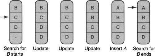
To reduce memory needs, update must work on the same binary search table on which search works. To insert element A in, say, Figure 15.5, update must move the elements B, C, and D one element down.
If the update and search designers are different, the normal specification for the update designer is always to ensure that the search process sees a consistent binary search table consisting of distinct keys. It appears to be very hard to meet this specification without allowing any search to take place until a complete update has terminated. Since an update can take a long time for a bridge database with 32,000 elements, this is unacceptable.
Thus, one could consider relaxing the specification (P3) to allow a consistent binary search table that contains duplicates of key values. After all, as long as the table is sorted, the presence of two or more keys with the same value cannot affect the correctness of binary search.
Thus the creation of a hole for A in Figure 15.5 is accomplished by creating two entries for D, then two entries for C, and then two entries for B, each with a single write to the table. In the last step, A is written in place of the first copy of B.
To keep the binary search chip simple (see Chapter 10), a route processor was responsible for updates while the chip worked on searches. The table was stored in a separate off-chip memory; all three devices (memory, processor, and chip) can communicate with each other via a common bus. Abstractly, separate search and update processes are concurrently making accesses to memory. Using locks to mediate access to the memory is infeasible because of the consequent slowdown of memory.
Given that the new specification allows duplicates, it is tempting to get away with the simplest atomicity in terms of reads and writes to memory. Search reads the memory and update reads and writes; the memory operations of search and update can arbitrarily interleave. Some implementors may assume that because binary search can work correctly even with duplicates, this is sufficient.
Unfortunately, this does not work, as shown in Figure 15.5.1 At the start of the scenario (leftmost picture), only B, C, and D are in the first, second, and third table entries. The fourth entry is free. A search for B begins with the second entry; a comparison with C indicates that binary search should move to the top half, which consists of only entry 1.
Next, search is delayed while update begins to go through the process of inserting A by writing duplicates from the bottom up. By the time update is finished, B has moved down to the second entry. When search finishes up by examining the first entry, it finds A and concludes (wrongly) that B is not in the table.
A simple attempt at reasoning correctly exposes this sort of counterexample directly. The standard invariant for binary search is that either the element being searched for (e.g., B) is in the current binary search range or B is not in the table. The problem is that update can destroy this invariant by moving the element searched for outside the current range.
In the bridge application, the only consequence of this failure is that a packet arriving at a known destination may get flooded to all ports. This will worsen performance only slightly but is unlikely to be noticed by external users!
15.3.2 Rescuing Reliability
A panic reaction to the counterexample of Figure 15.5 might be to jettison single-copy update and retreat to the safety of two copies. However, all the counterexample demonstrates is that a search must complete without intervening update operations. If so, the binary search invariants hold and correctness follows. The counterexample does not imply the converse: that an entire update must complete without intervening search operations. The converse property is restrictive and would considerably slow down search.
There are simple ways to ensure that a search completes without intervening updates. The first is to change the architectural model — algorithmics, after all, is the art of changing the problem to fit our limited ingenuity — so that all update writes are centralized through the search chip. When update wishes to perform a write, it posts the write to search and waits for an acknowledgment. After finishing its current search cycle, search does the required write and sends an acknowledgment. Search can then work on the next search task.
A second way, more consonant with the bridge implementation, is to observe that the route processor does packet forwarding. The route processor asks the chip to do search, and it waits for a few microseconds to get the answer. Finally, the route processor does updates only when no packets are being forwarded and hence no searches are in progress. Thus an update can be interrupted by a search, but not vice versa.
The final solution relies on search tolerating duplicates, and it avoids locking by changing the model to centralize updates and searches. Note that centralizing updates is insufficient by itself (without also relaxing the specification to allow duplicates) because this would require performing a complete update without intervening searches.
15.4 CONCLUSIONS
The routing protocol BGP (Border Gateway Protocol) controls the backbone of the Internet. In the last few years, careful scrutiny of BGP has uncovered several subtle flaws. Incompatible policies can lead to routing loops [VGE00], and attempts to make Internal BGP scale using route reflectors also lead to loops [GW02]. Finally, mechanisms to thwart instability by damping flapping routes can lead to penalizing innocent routes for up to an hour [MGVK02],
While credit must go to the BGP designers for designing a protocol that deals with great diversity while making the Internet work most of the time, there is surely some discomfort at these findings. It is often asserted that such bugs rarely manifest themselves in operational networks. But there may be a Three Mile Island incident waiting for us — as in the crash of the old ARPANET [Per92], where a single unlikely corner case capsized the network for a few days.
Even worse, there may be a slow, insidious erosion of reliability that gets masked by transparent recovery mechanisms. Routers restart, TCPs retransmit, and applications retry. Thus failures in protocols and router implementations may only manifest themselves in terms of slow response times, frozen screens, and rebooting computers.
Jeff Raskin says, “Imagine if every Thursday your shoes exploded if you tied them the usual way. This happens to us all of the time with computers, and nobody thinks of complaining.” Given our tolerance for pain when dealing with networks and computers, a lack of reliability ultimately translates into a decline of user productivity.
The examples in this chapter fit this thesis. In each case, incorrect distributed algorithm design leads to productivity erosion, not Titanic failures. Flow control deadlocks can be masked by router reboots, and cell loss can be masked by TCP retransmits. Failure to preserve ordering within an internal striping algorithm leads to TCP performance degradation, but not to loss. Finally, incorrect binary search table updates lead only to increased packet flooding. But together, the nickels and dimes of every reboot, performance loss, and unnecessary flood can add up to significant loss.
Thus this chapter is a plea for care in the design of protocols between routers and also within routers. In the quest for performance that has characterized the rest of the book, this chapter is a lonely plea for rigor. While full proofs may be infeasible, even sketching key invariants and using informal arguments can help find obscure failure modes. Perhaps if we reason together, routers can become as comfortable and free of surprises as an ordinary pair of shoes.
15.5 EXERCISES
1. FCVC Flow Control Protocol: The FCVC flow control protocol of Kung et al. [KCB94] provides an important alternative to the credit protocols described in Section 15.1. In the FCVC protocol, shown in Figure 15.6, the sender keeps a count of cells sent H while the receiver keeps a count of cells received R and cells dequeued D. The receiver periodically sends its current value of D, which is stored at the sender as estimate L. The sender is allowed to send if H – L > Max. More importantly, if the sender periodically sends H to the receiver, the receiver can deal with errors due to cell loss.
• Assume cells are lost and that the sender periodically sends H to the receiver. How can the receiver use the values of H and R to detect how many cells have been lost?
• How can the receiver use this estimate of cell loss to fix D in order to correct the sender?
• Can this protocol be made self-stabilizing without using the full machinery of a snapshot and reset?
• Compare the general features of this method of achieving reliability to the method used in the load-balancing algorithm described in the chapter.

2. Load Balancing with Variable-Size Packets: Load balancing within a router is typically at the granularity of cells. However, load balancing across routers is often at the granularity of (variable-sized) packets. Thus simple round-robin striping may not balance load equally because all the large packets may be sent on one link and the small ones on another. Modify the load-balancing algorithm without sequence numbers (using ideas suggested by the deficit round-robin (DRR) algorithm described in Chapter 14) to balance load evenly even while striping variable-size packets. Extend the fault-tolerance machinery to handle this case as well.
3. Concurrent Compaction and Search: In many lookup applications, routers must use available on-chip SRAM efficiently and may have to compact memory periodically to avoid filling up memory with unusably small amounts of free space. Imagine a sequence of N trie nodes of size-4 words that are laid out contiguously in SRAM memory after which there is a hole of size-2 words. As a fundamental operation in compaction, the update algorithm needs to move the sequence of N nodes two words to the right to fill the hole. Unfortunately, moving a node two steps to the right can overwrite itself and its neighbor. Find a technique for doing compaction for update with minimal disruption to a concurrent search process. Assume that when a node X is moved, there is at most one other node Y that points to X and that the update process has a fast technique for finding Y given X (see Chapter 11). Use this method to find a way to compact a sequence of trie nodes arbitrarily laid out in memory into a configuration where all the free space is at one end of memory and there are no “holes” between nodes. Of course, the catch is that the algorithm should work without locking out a concurrent search process for more than one write operation every K search operations, as in the bridge binary search example.