One of the key features of any report is the ability to display summary, or aggregate, information. For example, a sales report can show the overall sales total; sales subtotals by product type, region, or sales representatives; average sales figures; or the highest and lowest sales figures.
Aggregating data involves performing a calculation over a set of data rows. For a simple listing report, the aggregate calculations are performed over all the data rows in the report. The listing report in Figure 13-1 displays aggregate data at the end of the report.
In the example, BIRT calculates the average payment in the report by adding the payment amounts in every row, then dividing the total by the number of rows. Similarly, BIRT returns the largest and smallest payment amounts by comparing the payment amount in every row in the report.
For a report that groups data, as shown in Figure 13-2, you can display aggregates for each group of data rows, and for all the data rows in the report.
BIRT provides a wide range of functions in the Total class that support aggregate calculations over sets of data rows. These functions are custom JavaScript functions that BIRT defines. As with native JavaScript functions, you must use the correct capitalization when you type the function name, as shown in Table 13-1. For detailed information about each aggregate function, see Scripting Reference in BIRT’s online help.
Table 13-1. Aggregate functions
Aggregate function | Description |
|---|---|
Total.ave( ) | Returns the average value of a specified numeric field over all data rows. |
Total.count( ) | Counts the number of data rows in the set. |
Total.countDistinct( ) | Counts the number of unique values for a specified field. |
Total.first( ) | Returns the value of a specified field in the first data row. |
Total.isBottomN( ) | Returns a boolean value that indicates if the value of a specified numeric field is one of the bottom n values. |
Total.isBottomNPercent( ) | Returns a boolean value that indicates if the value of a specified numeric field is one of the bottom n percent values. |
Total.isTopN( ) | Returns a boolean value that indicates if the value of a specified numeric field is one of the top n values. |
Total.isTopNPercent( ) | Returns a boolean value that indicates if the value of a specified numeric field is one of the top n percent values. |
Total.last( ) | Returns the value of a specified field in the last data row. |
Total.max( ) | Returns the highest value of a specified field in the set of data rows. |
Total.median( ) | Returns the median, or mid-point, value for a set of values in a specified numeric field. |
Total.min( ) | Returns the lowest value of a specified field in the set of data rows. |
Total.mode( ) | Returns the mode, which is the value that occurs most often for a specified field. |
Total.movingAve( ) | Returns the moving average of a specified numeric field over a specified number of values. This type of calculation is typically used for analyzing trends of stock prices. |
Total.percentile( ) | Returns the percentile value for a set of values in a specified numeric field, given a specified percent rank. |
Total.percentRank( ) | Returns the rank of a number, string, or date-time value of a specified field as a percentage of the data set. The return value ranges from 0 to 1. |
Total.percentSum( ) | Returns the percentage of a total of a specified numeric field. |
Total.quartile( ) | Returns the quartile value for a set of values in a specified numeric field. |
Total.rank( ) | Returns the rank of a number, string, or date-time value of a specified field. |
Total.runningCount( ) | Returns the row number, up to a given point, in the report. |
Total.runningSum( ) | Returns the total, up to a given point, in the report. |
Total.stdDev( ) | Returns the standard deviation of a specified numeric field over a set of data rows. Standard deviation is a statistic that shows how closely values are clustered around the mean of a set of data. |
Total.sum( ) | Sums the values of a specified numeric field in the set of data rows. |
Total.variance( ) | Returns the variance of a specified numeric field over a set of data rows. Variance is a statistical measure of the spread of data. |
Total.weightedAve( ) | Returns the weighted average of a specified numeric field over a set of data rows. In a weighted average, some numbers carry more importance (weight) than others. |
Where you place aggregate data is essential to getting the correct results. For aggregate calculations, such as Total.sum( ), Total.ave( ), Total.max( ), and Total.mode( ), which process a set of data rows and return one value, you typically insert the aggregate data in the following places in a table:
At the beginning of a group, in the group header row
At the beginning of a table, in the header row
At the end of a group, in the group footer row
At the end of the table, in the footer row
You can place this type of aggregate data in a table’s detail row, but the data would not make much sense, because the same aggregate value would appear repeatedly for every row in the group. On the other hand, you typically insert aggregate calculations, such as Total.runningSum( ), Total.movingAve( ), Total.percentRank( ), and Total.Rank( ), in the detail row of a table. These functions process a set of data rows and return a different value for each row.
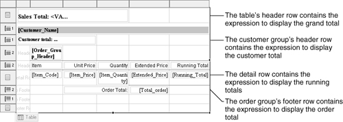
The report in Figure 13-3 groups data rows by customer, then by order ID. It displays totals for each order, totals for each customer, and a grand total of all sales. At the detail level, the report displays the running total for each line item.
To display the aggregate data as shown in the preceding report example, complete the following steps:
To display the grand total at the beginning of the report, place the aggregate data in the table’s header row.
To display the customer total at the beginning of each customer group, place the aggregate data in the customer group’s header row.
To display the order total at the end of each order group, place the aggregate data in the order group’s footer row.
To display the running totals, place the aggregate data in the table’s detail row.
Figure 13-4 shows the report design.
This section describes the expressions that you use to calculate the subtotals and totals that appear in the report example in the preceding section. As with all dynamic data, you define the aggregate expressions in a column binding. Then you insert a report element that uses the column binding.
To display the grand total in the table’s header, you can use either an HTML text element or a data element. Both elements enable you to use a combination of static text and dynamic data.
Text to use in an HTML text element:
Sales Total: <VALUE-OF format="$#.00">
Total.sum(row["Extended_Price"])</VALUE-OF>
Expression to use for a data element:
"Sales Total: $" + Total.sum(row["Extended_Price"]) +
   ".00"
Similarly, to display the customer total in the customer group’s header, you can use an HTML text element or a data element.
Text to use in an HTML text element:
Customer total: <VALUE-OF format="$#.00">
   Total.sum(row["Extended_Price"])</VALUE-OF>
Expression to use in a data element:
"Customer Total: $" + Total.sum(row["Extended_Price"]) +
   ".00"
To calculate and display the order total in the order group’s footer, use a data element. In this report example, a data element is more convenient, because only the dynamic value is necessary.
Total.sum(row["Extended_Price"])
To calculate and display the running totals in the detail row, use a data element and this expression:
Total.runningSum(row["Extended_Price"])
Notice that the group subtotals and report total are calculated with the same basic aggregate expression, Total.sum(row["Extended_Price"]). When you create multiple groups and place aggregate expressions in the headers or footers of various group levels, BIRT automatically calculates totals for the corresponding groups.
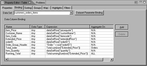
Figure 13-5 shows the column bindings defined for the table that contains all the report data. The Aggregate On values indicate the level at which aggregate calculations apply. The ALL value indicates that the aggregate calculation is applied to all rows in the table. The Orders value indicates that the aggregate calculation is applied to rows in the Orders group. The N/A value indicates that aggregation is not applicable, because the expression is not an aggregate expression.
Typically, you supply only a data set field (or a column binding that refers to a data set field) as an argument to an aggregate function, as shown in the following examples:
//Return the highest payment amount
Total.max(row["paymentAmount"])

//Return the lowest score
Total.min(row["score"])
//Return the average price
Total.ave(row["price"])

//Return the number of unique order IDs
Total.countDistinct(row["orderID"])

//Return the first date in the data set
Total.first(row["paymentDate"])

//Return the last name in the data set
Total.last(row["customerName"])
The exception is Total.count( ), which does not take a data set field as an argument. Total.count( ) returns the number of rows in a group or in the entire report, depending on where you place it.
If you use the expression builder to access the aggregate functions, these functions are listed under BIRT Functions—Total, as shown in Figure 13-6.
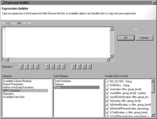
How to construct an aggregate expression in the expression builder
In Expression Builder, under Category, select BIRT Functions. Sub-Category displays the classes of functions that BIRT defines.
Select Total to display the aggregate functions.
Double-click the aggregate function that you want to use. The function appears in the expression area of Expression Builder.
Within the parentheses, ( ), of the function, specify the data set field, or column binding that refers to the data set field, whose values you want to aggregate:
Choose OK to save the expression.
When you calculate aggregate data, you can specify a filter condition to use to determine which rows are factored in the calculation. For example, you can exclude rows with missing or null credit limit values when you calculate an average credit limit or include only deposit transactions when you calculate the sum of transactions.
To specify a filter condition when you aggregate data, specify a filter expression that evaluates to true or false. Include the filter expression as an argument to the aggregate function. You specify the filter expression either as the second or third argument, depending on the function. The exception is Total.count( ), where the filter expression is the first argument, because this function does not reference a data set field.
The following expressions are examples of aggregate expressions that include a filter condition:
This expression returns the sum of extended prices for item MSL3280 only:
Total.sum(row["extendedPrice"], row["itemCode"]=="MSL3280")
This expression returns the average order amount for closed orders only:
Total.ave(row["orderAmount"], row["orderStatus"]=="Closed")
This expression returns the number of rows in a group or a table (depending on where you place the expression) and counts only rows where the order amount exceeds $10:
Total.count(row["orderAmount"] > 10)
When you calculate the sum of a numeric field, it does not matter if some of the rows contain null values for the specified numeric field. The results are the same, regardless of whether the calculation is 100 + 75 + 200 or 100 + 75 + 0 (null) + 200. In both cases, the result is 375. Note that null is not the same as zero (0). Zero is an actual value, whereas null means there is no value.
Some aggregate calculations return different results when null values are included or excluded from the calculation. The average value returned by the calculation without the null value in the previous example is 125 ((100 + 75 + 200)/3). The average value of the calculation with the null value, however, is 93.75 ((100 + 75 + 0 + 200)/4). Similarly, Total.count( ) returns a different number of total rows, depending on whether you include or exclude rows with null values for a specified field.
By default, aggregate functions include all rows in their calculations. To exclude null values, you must specify a filter condition. The following expressions are examples of aggregate expressions that filter out rows that contain null values in specified fields:
This expression returns the average transaction amount. The calculation includes only rows in which the transaction amount is not null.
Total.ave(row["transactionAmount"],
    row["transactionAmount"] != null)
This expression returns the total number of rows in a group or a table, excluding rows in which the creditLimit field has no value. Here, the filter expression is the first argument, because Total.count( ), unlike the other aggregate functions, does not reference a data set field.
Total.count(row["creditLimit"] != null)
When you use Total.count( ) to return the number of rows in a group or table, BIRT counts all rows. Sometimes, you want to get the count of distinct values. For example, a table displays a list of customers and their countries, as shown in Figure 13-7. The table lists 12 customers from 4 different countries.
Table 13-7. A table that lists customers and their countries
Customers with orders over 10K | |
Customer | Country |
American Souvenirs | USA |
Land of Toys Inc. | USA |
Porto Imports | |
La Rochelle Gifts | France |
Gift Depot | USA |
Dragon Souvenirs | Singapore |
Saveley & Henriot, Co. | France |
Technics Stores Inc. | USA |
Osaka Souvenirts Co | Japan |
Diecast Classics Inc | USA |
Collectable Mini Designs | USA |
Mini Wheels Co | USA |
If you insert a data element that uses the expression Total.count( ) in the header or footer row of the table, Total.count( ) returns 12, the number of rows in the table. If, however, you want to get the number of countries, use Total.countDistinct( ), as shown in the following expression:
Total.countDistinct(row["country"])
In the example report, Total.countDistinct() returns 5, not 4 as you might expect, because like the other aggregate functions, Total.countDistinct() counts rows with null values. The third row in the table contains a null value for country. To get the real count of countries that are listed in the table, add a filter condition to the aggregate expression, as follows:
Total.countDistinct(row["country"], row["country"] != null)
This expression counts only rows in which the country value is unique and not null.
As the example report in “Placing aggregate data,” earlier in this chapter shows, you typically insert an aggregate expression in the header or footer of a group to calculate and show aggregate information for that particular group. For example, to calculate the sum of orders for each customer, you insert an expression, such as Total.sum(row[“extendedPrice”]), in the header of the customer group to display the information at the beginning of each customer group or in the footer to display the information at the end of each customer group.
Sometimes, however, you might want to display an aggregate value from a different group. The report shown in Figure 13-8 displays the grand total (the sum of all customer orders) in each customer group.
The Total.sum(row[“extendedPrice”]) expression in the customer group calculates the sum of extended prices over all data rows in the customer group only. The overall total, however, is calculated over all the data rows in the report’s data set.
To display the overall total in the customer group header, you must specify the group for which you want an aggregate value. You accomplish this task in either of the following ways:
In the column-binding definition, specify the following expression, and set Aggregate On to ALL:
Total.sum(row["extendedPrice"])
In the column-binding definition, specify the following expression:
Total.sum(row["extendedPrice"], null, "overall")
The key piece of this expression is the value that you supply as the third argument to the Total.sum( ) function. The value “overall” refers to the overall total for all the rows in the data set. This value overrides the value set for Aggregate On. Note that, because you need to supply a value for the third argument, you need to also specify a value for the second argument, which takes a filter condition. The example uses the null value, because a filter is not required. Filtering aggregate data is described earlier in this chapter.
Similarly, if you want to display the customer total in the order ID group, you can accomplish the task using either of the following ways:
Specify the following expression, and set Aggregate On to Customers:
Total.sum(row["extendedPrice"])
Specify the following expression:
Total.sum(row["extendedPrice"], null, "Customers")
If you use the second method, you can supply different types of values for the third argument. For example, you can specify the group index instead of the group name. In our example, the Customers group is the first group, so its index is 1. An index value of 0 gets the overall total. For example, the following expressions return the same results:
Total.sum(row["extendedPrice"], null, "Customers")
Total.sum(row["extendedPrice"], null, 1)
The following expressions also return the same results:
Total.sum(row["extendedPrice"], null, "overall")
Total.sum(row["extendedPrice"], null, 0)
The ability to access the aggregate value from any group of data in the report is useful. Not only can you display the values, you can use them in calculations that require aggregate values from multiple groups. Percentage calculations, for example, require a subtotal and an overall total. Information about calculating percentages is in the following section.
Some percentage calculations require aggregate values from two different groups of data. For example, a report displays each regional sales total as a percentage of the total national sales. To calculate this aggregate data for each region, two totals are required:
The total of all sales in each region.
The overall total of sales across all regions.
Figure 13-9 shows an example of a report that displays sales data that is grouped by state, then by product. The report shows two percentage calculations:
A state’s total sales as a percentage of the overall sales.
A product’s total sales as a percentage of the state’s total sales.
Figure 13-10 shows the report design.
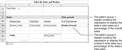
To calculate this percentage for the report design shown in Figure 13-10, specify the following expression for a column binding whose Aggregate On value is set to Product:
Total.sum(row["extendedPrice"])/
   Total.sum(row["extendedPrice"], null, "State")
As the previous section describes, you obtain the aggregate value of another group by specifying the name of the group. In this example, the value “State” identifies the group whose total you want. The second argument is null, which means that there is no filter.
Alternatively, you can create three column bindings, one for each discrete piece of the calculation. The first column binding defines the expression to calculate the product total:
Total_Product: Total.sum(row["extendedPrice"])
Aggregate On Product
The second column binding defines the expression to calculate the state total:
Total_State: Total.sum(row["extendedPrice"])
Aggregate On State
The third column binding defines the expression to calculate the percentage. This expression refers to the previous column bindings, Total_Product and Total_State.
Product_Percent: row["Total_Product"]/row["Total_State"]
Aggregate On N/A
To calculate this percentage for the report design shown in Figure 13-10, specify the following expression for a column binding whose Aggregate Value is set to State:
Total.sum(row["extendedPrice"])/
   Total.sum(row["extendedPrice"], null, "overall")
The value “overall” specifies the overall total for the entire data set.
Alternatively, you can create three column bindings, one for each discrete piece of the calculation. The first column binding defines the expression to calculate the state total:
Total_State: Total.sum(row["extendedPrice"])
Aggregate On State
The second column binding defines the expression to calculate the overall total:
Total_All: Total.sum(row["extendedPrice"])
Aggregate On ALL
The third column binding defines the expression to calculate the percentage:
State_Percent: row["Total_State"]/row["Total_All"]
Aggregate On N/A
The values returned by the previous calculations range from 0 to 1. To display a value, such as 0.8, as 80%:
Reports typically display both detail and aggregate data. A summary report is a report that shows only aggregate data. Summary reports, such as the top ten products or sales totals by state, provide key information at a glance and are easy to create.
When you create a report that contains data in detail rows and aggregate data in header or footer rows, you can change such a report to a summary report by hiding the contents in the detail rows. To hide these contents, you can use any of the following techniques:
Choose the group whose detail rows you want to hide, and in the group editor, select the Hide Detail option.
Select the detail row, and use the visibility property should be init cap to hide the contents of the row.
Delete the contents from the detail row. A report does not need to display the values of the data rows to perform aggregate calculations on the data rows.
The first and second techniques provide the flexibility of maintaining two versions of a report. The third technique, on the other hand, results in a summary report only. To change the report to display details, you would have to add the data back to the detail row.
Take a closer look at the report design in Figure 13-10. The report contains data only in the header and footer rows, and almost all the data elements display totals. Rather than display individual sales records in the detail rows, the report shows only the sales total for each product.
To create a top n or bottom n summary report, insert the aggregate data in the header or footer row. Then create a filter for the group that contains the data, and use a filter condition, as shown in the following examples:
//Show only the top ten orders
Total.sum(row["extendedPrice"]) Top n 10

//Show only orders in the top ten percent
Total.sum(row["extendedPrice"]) Top Percent 10

//Show only the lowest five orders
Total.sum(row["extendedPrice"]) Bottom n 5

//Show only orders in the bottom one percent
Total.sum(row["extendedPrice"]) Bottom Percent 1
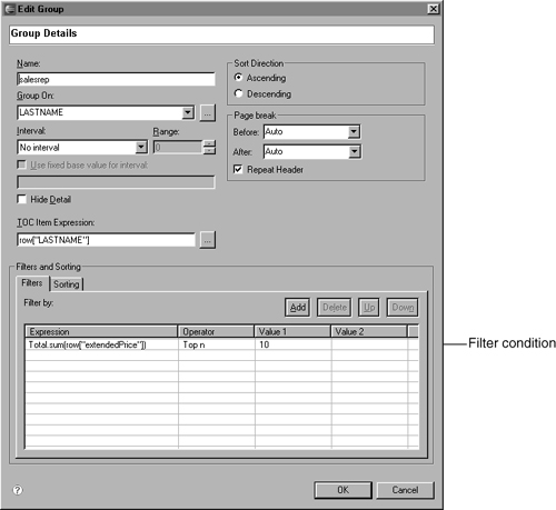
Figure 13-11 shows a top ten report. Figure 13-12 shows the report design.
The data elements that display the sales representative names and their sales totals are in a group header row. This report groups sales data rows (not shown in the report) by sales representatives. To display only the top ten sales representatives, a filter is in the group definition, as shown in Figure 13-13.