When we explored BFS, we saw that it was able to solve the shortest path problem for unweighted graphs, or graphs whose edges have the same (positive) weight. What if we are dealing with weighted graphs? Can we do better? We shall see that Dijkstra's algorithm provides an improvement over the ideas presented in BFS and that it is an efficient algorithm for solving the single-source shortest path problem. One restriction for working with Dijkstra's algorithm is that edges' weights have to be positive. This is usually not a big issue since most graphs represent entities modeled by edges with positive weights. Nonetheless, there are algorithms capable of solving the problem for negative weights. Since the use case for negative edges is less common, those algorithms are outside the scope of this book.

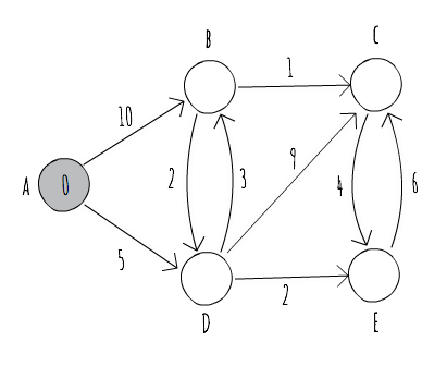
Dijkstra's algorithm, conceived by Edsger W. Dijkstra in 1956, maintains a set S of vertices whose final shortest-path weights from the source s have already been determined. The algorithm repeatedly selects the vertex u with the minimum shortest-path estimate, adds it to set S, and uses the outward edges from that vertex to update the estimates from vertices not yet in set S. In order to see this in action, let's consider the directed graph of Figure 6.5:

The graph is composed of five vertices (A, B, C, D, and E) and 10 edges. We're interested in finding the shortest paths, starting at vertex A. Note that A is already marked as 0, meaning that the current distance from A to A is zero. The other vertices don't have distances associated with them yet. It is common to use an estimate of infinity as the starting estimate for the distance of nodes not yet seen. The following table shows a run of Dijkstra's algorithm for the graph of Figure 6.5, identifying the current vertex being selected and how it updates the estimates for vertices not yet seen:

Step	Explanation
	Vertex A is the vertex with the lowest estimate weight, so it is selected as the next vertex whose edges are to be considered to improve our current estimates.
	We use the outward edges from vertex A to update our estimates for vertices B and D. Afterwards, we add A to set S, avoiding a repeated visit to it. From the edges not yet visited, the one with the lowest estimate is now D, which shall be selected to visit next. Note that we also mark those edges that belong to our estimate shortest path in bold.
	By exploring the outward edges from vertex D, we were able to improve our estimate for vertex B, so we update it accordingly and now consider a different edge for the shortest path. We were also able to discover vertices C and E, which become potential candidates to visit next. Since E is the one with the shorter estimate weight, we visit it next.
	Using an outward edge from vertex E, we were able to improve our estimate for vertex C, and now look at vertex B as our next vertex to visit. Note that those vertices that belong to set S (shown in black in the figure) already have their shortest path computed. The value inside them is the weight of the shortest path from A to them, and you can follow the edges in bold to build the shortest path.
	From vertex B, we were able to once again improve our estimate for the shortest path to vertex C. Since vertex C is the only vertex not yet in set S, it is the one visited next.
	Since vertex C has no outward edges to vertices not yet in S, we conclude the run of our algorithm, and have successfully computed the shortest paths from A to every other vertex in the graph.

Now that we've seen a run of Dijkstra's algorithm, let's try to put it in code and analyze its runtime performance. We will use an adjacency list representation for our graph, as it helps us when trying to explore the outward edges of a given vertex. The following code snippet shows a possible implementation of Dijkstra's algorithm as previously described:

while (!notVisited.isEmpty()) {
  Vertex v = getBestEstimate(notVisited);
  notVisited.remove(v);
  visited.add(v);
  for (Edge e : adj[v.u]) {
    if (!visited.contains(e.v)) {
      Vertex next = vertices[e.v];
      if (v.distance + e.weight < next.distance) {
        next.distance = v.distance + e.weight;
        parent[next.u] = v.u;
      } 
    }
  } 
}  

The Dijkstra method starts by initializing two sets:

• One for visited vertices
  
• One for unvisited vertices

The set of visited vertices corresponds to the set we previously named as S, and we use the one of not visited vertices to keep track of vertices to explore.

We then initialize each vertex with an estimated distance equal to Integer.MAX_VALUE, representing a value of "infinity" for our use case. We also use a parent array to keep track of parent vertices in the shortest path, so that we can later recreate the path from the source to each vertex.

The main loop runs for each vertex, while we still have vertices not yet visited. For each run, it selects the "best" vertex to explore. In this case, the "best" vertex is the one with the smallest distance of the vertices not visited so far (the getBestEstimate() function simply scans all vertices in the notVisited() set for the one satisfying the requirement).

Then, it adds the vertex to the set of visited vertices and updates the estimate distances for not visited vertices. When we run out of vertices to visit, we build our paths by recursively visiting the parent array.

Analyzing the runtime of the previous implementation, we can see that we have an initialization step that's proportional to the number of vertices in the graph, hence running in O(V).

The main loop of the algorithm runs once for each vertex, so it is bounded by at least O(V). Inside the main loop, we determine the next vertex to visit and then scan its adjacency list to update the estimate distances. Updating the distances takes time proportional to O(1), and since we scan each vertex's adjacency list only once, we take time proportional to O(E), updating estimate distances. We're left with the time spent selecting the next vertex to visit. Unfortunately, the getBestEstimate() method needs to scan through all the unvisited vertices, and is therefore bounded by O(V). The total running time of our implementation of Dijkstra's algorithm is therefore O(V²+E).

Even though some parts of our implementation seem difficult to optimize, it looks like we can do better when selecting the next vertex to visit. If we could have access to a data structure that was capable of storing our vertices sorted by lower estimated distance and provided efficient insert and remove operations, then we could reduce the O(V) time spent inside the getBestEstimate method.

In Chapter 4, Algorithm Design Paradigms, we briefly discussed a data structure used in Huffman coding named the  priority queue, which is just what we need for this job. The following code snippet implements a more efficient version of Dijkstra's algorithm, using a priority queue:

PriorityQueue<Node> pq = new PriorityQueue<>();
pq.add(new Node(source, 0));
while (!pq.isEmpty()) {
  Node v = pq.remove();
  if (!vertices[v.u].visited) {
    vertices[v.u].visited = true;
    for (Edge e : adj[v.u]) {
      Vertex next = vertices[e.v];
      if (v.distance + e.weight < next.distance) {
        next.distance = v.distance + e.weight;
        parent[next.u] = v.u;
        pq.add(new Node(next.u, next.distance));
      }
    }
  } 
} 

In this second implementation, we no longer keep sets for visited and not visited vertices. Instead, we rely on a priority queue that will be storing our distance estimates while we run the algorithm.

When we are exploring the outward edges from a given vertex, we therefore add a new entry to the priority queue in case we are able to improve our distance estimate.

Adding and removing an element from our priority queue takes O(logN) time, N being the number of elements in the queue. Do note that we can have the same vertex inserted more than once in the priority queue. That's why we check if we've visited it before expanding its edges.

Since we will visit the instance for that vertex with shorter estimate distance, it's safe to ignore the ones that come after it. However, that means that operations on our priority queue are not bounded by O(logV), but O(log E) instead (assuming that there's a connected graph).

Therefore, the total runtime of this implementation is O((V + E)logE). It's still possible to improve this running time by using a priority queue implementation with better asymptotic bounds (such as a Fibonacci heap), but its implementation is out of the scope of this book.

One last thing to note about Dijkstra's algorithm is how it borrows ideas from BFS (the algorithm structure is very similar to Dijkstra's, but we end up using a priority queue instead of a normal queue) and that it is a very good example of a greedy algorithm: Dijkstra's algorithm makes the locally optimum choice (for example, it chooses the vertex with the minimum estimated distance) in order to arrive at a global optimum.