
To better understand algorithmic complexity, we can make use of an analogy. Imagine that we were to set different types of algorithms so that they compete against one another on a race track. However, there is a slight twist: The race course has no finish line.
Since the race is infinite, the aim of the race is to surpass the other, slower opponents over time and not to finish first. In this analogy, the race track distance is our algorithm input. How far from the start we get, after a certain amount of time, represents the amount of work done by our code.
Recall the quadratic method for measuring the closest pair of planes in the preceding section. In our fictitious race, the quadratic algorithm starts quite fast and is able to move quite a distance before it starts slowing down, similar to a runner that is getting tired and slowing down. The further it gets away from the start line, the slower it gets, although it never stops moving.
Not only do the algorithms progress through the race at different speeds, but their way of moving varies from one type to another. We already mentioned that O(n2) solutions slow down as they progress along the race. How does this compare to the others?
Another type of runner taking part in our imaginary race is the linear algorithm. Linear algorithms are described with the notation of O(n). Their speed on our race track is constant. Think of them as an old, reliable car moving at the same fixed speed.
In real life, solutions that have an O(n) runtime complexity have a running performance that is directly proportional to the size of their input.
This means, for example, that if you double the input size of a linear algorithm, the algorithm would also take about twice as long to finish.
The efficiency of each algorithm is always evaluated in the long run. Given a big enough input, a linear algorithm will always perform better than a quadratic one.
We can go much quicker than O(n). Imagine that our algorithm is continually accelerating along the track instead of moving constantly. This is the opposite of quadratic runtime. Given enough distance, these solutions can get really fast. We say that these type of algorithms have a logarithmic complexity written as O(log n).
In real life, this means that the algorithm doesn't slow much as the size of the input increases. Again, it doesn't matter if at the start, the algorithm performs slower than a linear one for a small input, as for a big enough input, a logarithmic solution will always outperform the linear one.
Can we go even faster? It turns out that there is another complexity class of algorithms that performs even better.
Picture a runner in our race who has the ability to teleport in constant time to any location along our infinite track. Even if the teleportation takes a long time, as long as it's constant and doesn't depend on the distance traveled, this type of runner will always beat any other. No matter how long the teleportation takes, given enough distance, the algorithm will always arrive there first. This is what is known as a constant runtime complexity, written as O(1). Solutions that belong to this complexity class will have a runtime independent of the input size given.
On the other side of the spectrum, we can find algorithms that are much slower than quadratic ones. Complexities such as cubic with O(n3) or quartic with O(n4) are examples. All of the mentioned complexities up to this point are said to be polynomial complexities.
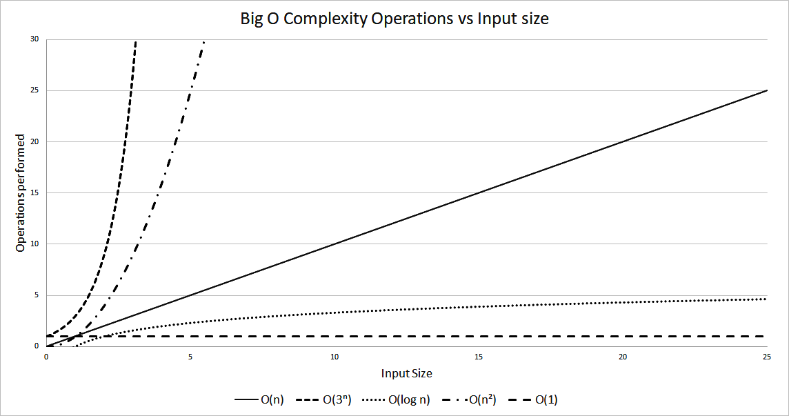
Not all solutions have a polynomial time behavior. A particular class of algorithms scale really badly in proportion to their input with a runtime performance of O(kn). In this class, the efficiency degrades exponentially with the input size. All the other types of polynomial algorithms will outperform any exponential one pretty fast. Figure 1.2 shows how this type of behavior compares with the previously mentioned polynomial algorithms.
The following graph also shows how fast an exponential algorithm degrades with input size:
How much faster does a logarithmic algorithm perform versus a quadratic one? Let's try to pick a particular example. A specific algorithm performs about two operations to solve a problem; however, the relation to its input is O(n2).
Assuming each operation is a slow one (such as file access) and has a constant time of about 0.25 milliseconds, the time required to perform those operations will be as shown in Table 1.3. We work out the timings by Time = 0.25 * operations * n2, where operations is the number of operations performed (in this example it's equal to 2), n is the input size, and 0.25 is the time taken per operation:
| Input Size (n) | Time: 2 operations O(n2) | Time: 400 operations O(log n) |
| 10 | 50 milliseconds | 100 milliseconds |
| 100 | 5 seconds | 200 milliseconds |
| 1000 | 8.3 minutes | 300 milliseconds |
| 10000 | 13.8 hours | 400 milliseconds |
Our logarithmic algorithm performs around 400 operations; however, its relation to the input size is logarithmic. Although this algorithm is slower for a smaller input, it quickly overtakes the quadratic algorithm. You can notice that, with a large enough input, the difference in performance is huge. In this case, we work out the timing using Time = 0.25 * operations * log n, with operations = 400.