In the previous section, we saw how we can deal with collisions using linked lists at each array position. A chained hash table will keep on growing without any load limit. Open addressing is just another way of tackling hash collisions. In open addressing, all items are stored in the array itself, making the structure static with a maximum load factor limit of 1. This means that once the array is full, you can't add any more items. The advantage of using open addressing is that, since you're not using linked lists, you're saving a bit of memory since you don't have to store any pointer references.

You can then use this extra memory to have an even larger array and hold more of your key value pairs. To insert in an open-addressed hash table, we hash the key and simply insert the item in the hash slot, the same as a normal hash table. If the slot is already occupied, we search for another empty slot and insert the item in it. The manner in which we search for another empty slot is called the probe sequence.

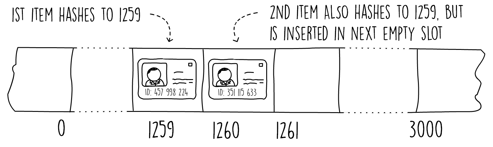
A simple strategy, shown in Figure 3.5, is to search by looking at the next available slot. This is called linear probing, where we start from the array index at the hash value and keep on increasing the index by one until we find an empty slot. The same probing technique needs to be used when searching for a key. We start from the hash slot and keep on advancing until we match the key or encounter an empty slot:

The next code snippet shows the pseudocode for linear probing insert. In this code, after we find the hash value we keep on increasing a pointer by one, searching for an empty slot.

Once we reach the end of the array, we wrap around to the start using the modulus operator. This technique is similar to one we used when we implemented array-based stacks. We stop increasing the array pointer either when we find a null value (empty slot) or when we get back to where we started, meaning the hash table is full. Once we exit the loop, we store the key-value pair, but only if the hash table is not full.

The pseudocode is as follows:

insert(key, value, array)
  s = length(array)
  hashValue = hash(key, s)
  i = 0
  while (i < s and array[(hashValue + i) mod s] != null)
    i = i + 1
  if (i < s) array[(hashValue + i) mod s] = (key, value)  

Searching for a key is similar to the insert operation. We first need to find the hash value from the key and then search the array in a linear fashion until we encounter the key, find a null value, or traverse the length of the array.

If we want to delete items from our open, addressed hash table, we cannot simply remove the entry from our array and mark it as null. If we did this, the search operation would not be able to check all possible array positions for which the key might have been found. This is because the search operation stops as soon as it finds a null.

One solution is to add a flag at each array position to signify that an item has been deleted without setting the entry to null. The search operation can then be modified to continue past entries marked as deleted. The insert operation also needs to be changed so that, if it encounters an entry marked as deleted, it writes the new item at that position.

Linear probing suffers from a problem called clustering. This occurs when a long succession of non-empty slots develop, degrading the search and insert performance. One way to improve this is to use a technique called quadratic probing. This strategy is similar to linear probing, except that we probe for the next empty slot using a quadratic formula of the form h + (ai + bi²), where h is the initial hash value, and a and b are constants. Figure 3.6 shows the difference between using linear and quadratic probing with a = 0 and b = 1. The diagram shows the order in which both techniques explore the array.

In quadratic probing, we would change Snippet 3.3 to check at array indexes of the following:

 array[(hashValue + a*i + b*i^2) mod s] 

One other probing strategy used in open-addressing hash tables is called double hashing. This makes use of another hash function to determine the step offset from the initial hash value. In double hashing, we probe the array using the expression h + ih'(k), where h is the hash value and h'(k) is a secondary hash function applied on the key. The probing mechanism is similar to linear probing, where we start with an i of zero and increase by one on every collision. Doing so results in probing the array every h'(k) step. The advantage of double hashing is that the probing strategy changes on every key insert, reducing the chances of clustering.

In double hashing, care must be taken to ensure that the entire array is explored. This can be achieved using various tricks. For example, we can size our array to an even number and make sure the secondary hash function returns only odd numbers.