
5
Deep Learning Architectures for IoT Data Analytics
Snowber Mushtaq1 and Omkar Singh2
1 Department of Computer Science and Engineering, Islamic University of Science and Technology, Jammu and Kashmir, India
2 Department of Electronics and Communication Engineering, National Institute of Technology, Srinagar, India
5.1 Introduction
Internet of Things (IoT) has evolved as a modern research area because of the increased connected devices. This allows multiple devices to connect over a network without human intervention. It has evolved due to the merging of multiple technologies that has been deployed in various fields of day‐to‐day life, including smart home, elderly care to provide support to elder and physically challenged people, and also toward the commercial applications. IoT is a concept that allows objects to communicate with each other, operate in co‐ordination with additional things to create novel applicability, and attain mutual targets [1]. Every connected device must be considered a thing, in terms of IoT. Things can be any physical sensors, actuators, and an embedded system with a microprocessor. Data collected from sensors deployed in IoT can be used to understand, monitor, and control complex environments around us, promoting greater intellect, more forward decision‐making, and more reliable performance [2]. Entities communicate with each other, known as a device‐to‐device communication. Individual communication can either be short‐range or long‐range. Short‐range communication can be realized practicing wireless technologies such as Wi‐Fi, Bluetooth, and ZigBee, and wide‐range has achieved using mobile networks such as WiMAX, GSM, GPRS, 3G, 4G, LTE, and 5G. The commercial applications of IoT include medical health, transportation, industrial applications, etc. Artificial Intelligence is presently a part of IoT considering it helps in automated processing, control of devices, and produces promising results. A significant number of connected devices are increasing exponentially, and it is expected to grow around 75 billion by 2025. Thus, data management clarifications are needed for efficient management and transmission of data. ML has provided a way to the management of a large volume of data [3]. The leading success of DL contributed a new direction to tackle problems related to the administration of space. That has the property to categorize a large volume of data sent and received by devices. DL renders support to a large sensor data for effective learning of underlying features in intelligent devices. Explicit merge of IoT and DL has provided new applications of IoT including disease analysis, health monitoring, intelligent control of various appliances, robots, traffic analysis and prediction, and autonomous driving [4]. Big data is the advanced analytical method for better prediction and manipulation of large dimensions of data. DL has been deployed for an end‐to‐end delivery of reliable noise‐free data in IoT.
DL is on inflation from the recent time, and it is there to stay for about a decade of now. The manufacturers are using DL algorithms to generate more income. They are training their workers to learn this experience and contribute to their firm. A lot of startups are beginning up with innovative DL resolutions that can solve challenging puzzles. Also in academia, a lot of investigation is taking place each day, and the way DL is transforming the world entirely is mind‐boggling. The DL structures have produced much better than contemporary methods and have achieved the best performances. Thus, to survive in either industry or academia possessing DL skills will most likely play an important role in the advancing years.
Artificial Intelligence is the field of modern computer science that simulates human brain functions, generally problem‐solving and learning. It simulates human intellect in machines and is based on the ethic that it can start from simple to complex problem execution. It has been deployed in endless fields including finance, healthcare, etc. Artificial Intelligence has impacted various day‐to‐day activities providing security, verification, and validity. This learns from experiences and adjusts the inputs to perform intelligent tasks. One adds intelligence by discovery, extracts deeper into data with accuracy, and extracts most valuable information out of data. ML is a subfield of Artificial Intelligence or an application of Artificial Intelligence that makes a machine intelligent without being directly programmed and earns experience or performance over time. This focuses on automated learning without human involvement. Moreover, it can identify patterns, make decisions, and build analytical models automatically. ML algorithms are classified into supervised, unsupervised, semi‐supervised, and reinforcement algorithms. DL is a subfield of ML, also known as deep neural networks or deep neural learning. DL has gained popularity nowadays due to the improvement in ML and advancement in chip processing [5]. Hither utilizes a stratified level of artificial neural networks to carry out the processing. DL uses the underlying neural network architecture so‐known as deep neural networks. Neural networks are inspired by biological neurons that are the basic structure in the human and animal brain. Neural networks can gain experience by storing it and practicing. It is similar to the human brain where the connections are between the neurons, and the connection strength between the neurons determines the knowledge. Deep Neural architectures have more than one hidden layer. Single‐layer neural networks have one hidden layer of neurons and are used to solve linearly separable problems. That is, there is a single hyperplane to divide the input data into two separate classes. Solving the XOR problem is a classical neural network problem where the XOR's input cannot be separated by a single line. Hence, multilayer neural networks are used to solve problems like linearly inseparable ones. DL has more number of layers to extract more depth of features. The next layer extracts more depth features based on the previous layer. DL can handle high dimensional and complex unstructured data like text, video, pictures, etc. This has the ability to learn from different sources of data and to handle a large volume of data [6]. It has more significant learning and prediction ability than ML. They have hierarchical structures for connection between different layers. DL models are more robust than ML in terms of the extraction of features. Some popular DL architectures include restricted Boltzmann machine (RBM), deep belief networks (DBN), autoencoders (AE), convolutional neural networks (CNN), recurrent neural networks (RNN), long short‐term memory (LSTM), etc.
Figure 5.1 explains the relationship between DL and Artificial intelligence. Learning algorithms in Artificial Intelligence use computational methods to learn directly from data without relying on a predestined comparison as a standard. The algorithms advance their performance as the number of examples available for learning increases. DL is a specific form of ML. In learning algorithms, we have a set of examples called training set as input data, and we have to predict the output set.
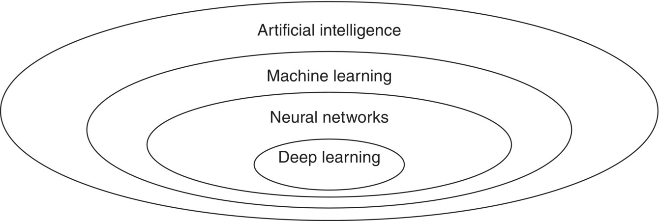
Figure 5.1 Deep neural networks in the context of artificial intelligence.
5.1.1 Types of Learning Algorithms
We mainly have four broad categories of learning algorithms.
5.1.1.1 Supervised Learning
In supervised learning, the training set is provided with a set of labels to predict the target value. Its main application includes regression (target values are continuous values) such as predicting weather and population growth. Additionally, it can also be applied to classification problems like speech recognition, fraud detection, digit recognition, diagnostics, etc., by employing algorithms like support vector machine (SVM), random forest, and others. Learning here is divided into two parts. (i) Training phase: Here the data is provided with a label, and the algorithm learns the relationship between input data and labels and determines the output for the test data. (ii) Testing phase: Here the data without a label is provided as input, and the algorithm finds the relationship between input data and previous labels and determines the output for the test data [7].
5.1.1.2 Unsupervised Learning
In unsupervised learning training, a set is not provided with a set of labels. This is meant for finding useful structures or knowledge in data when no labels are available. It is also used in detecting abnormal server access patterns, detecting irregular access to websites, outlier detection, social network analysis, organizing computing clusters, etc. It solves clustering problems like target marketing, customer segmentation, and recommendation system. It also tries to find patterns to predict future values and also applied for dimensionality reduction problems.
5.1.1.3 Semi‐Supervised Learning
It is a combination of supervised and unsupervised learning, that is, both labeled and unlabeled data are used. This is an improvement over unsupervised learning [8].
5.1.1.4 Reinforcement Learning
In reinforcement learning, appropriate steps or a sequence of steps are to be taken for a given situation to maximize the payoff. Its applications include AI gaming, real‐time decisions, skill acquisition, and robot navigation. Figure 5.2 explains broad categories of learning.
5.1.2 Steps Involved in Solving a Problem
Framework flow to solve a problem:
- Problem Definition: Understand the problem simply that is being solved and describe it.
- Analyze Data: Understand all the data accessible for solving the problem.
- Prepare Data: Prepare the structure of the dataset from previous data.
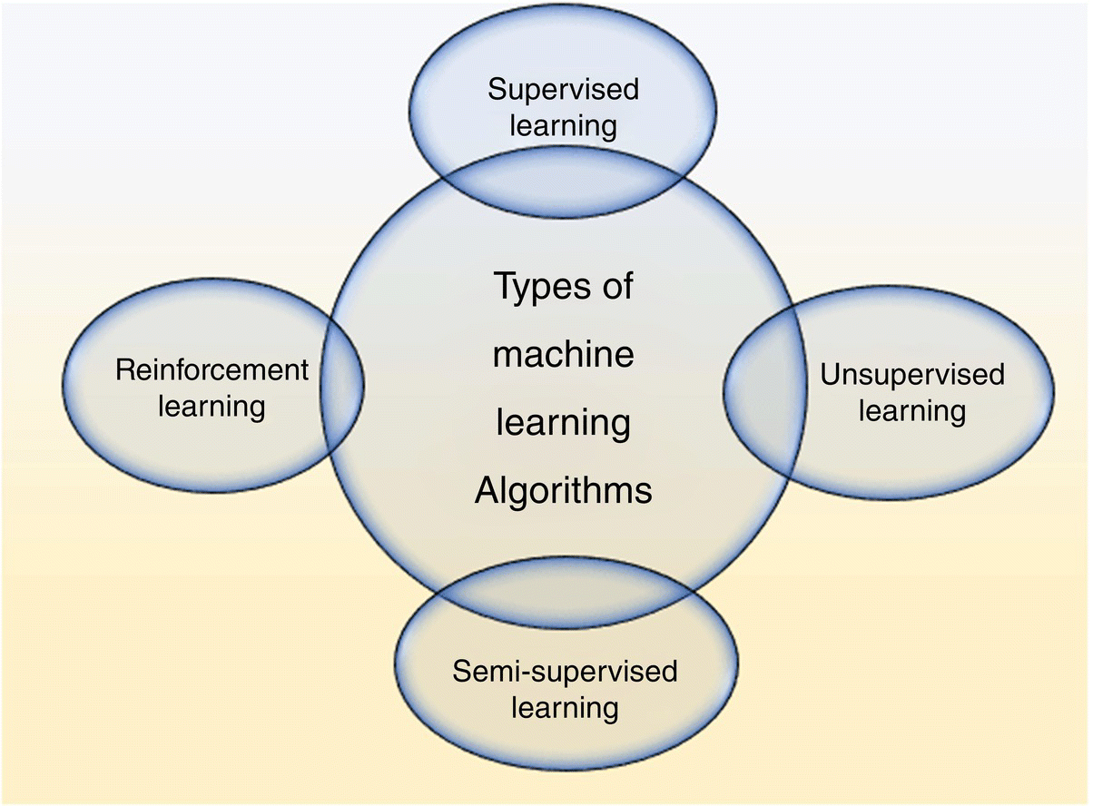
Figure 5.2 Types of learning algorithms.
- Evaluate Algorithm: Develop some baseline precision from which to improve.
- Improve Results: Support results to confirm a more perfect model.
- Present Result: Explain the solution so that it can be understood by users.
5.1.2.1 Basic Terminology
- Representation: understand the problem
- Evaluation: find effectiveness
- Optimization: solve the problem and feature representation.
5.1.2.2 Training Process
The training set consists of N training samples labeled as {( xi, yi), …( xm, ym)}. ( xi, yi) is a training instance. xi is the ith m‐dimensional input vector, yi is the ith n‐dimensional output vector. x = {x1, x2, . . , xm} is the m‐dimensional input matrix and y = {y1, y2, . . , yn} is the n‐dimensional output matrix. Artificial Intelligence techniques build a model from the input and map its corresponding output until the system stabilizes.
5.1.3 Modeling in Data Science
Modeling is done whenever we have to understand any part of the science whether it is physics, chemistry, mathematics, etc. For better understanding and representation of concepts, a model is created and is used to generate an idea and test the theories. Modeling in data science consists of two main categories: (i) Generative and (ii) Discriminative.
5.1.3.1 Generative
In the case of Generative models, individual class distribution is modeled. The Generative models are based on joint probability distribution p(x, y) = p(y) * p(y ∣ x) and conclude based on Bayes rule and select the most likely label. When conditional independence is not convinced, they prove less accurate. They need fewer data to train and test well when working with missing data. They are applied to find hidden parameters and are used for solving classification problems. Generative models have less chance to overfit but are affected by outliers and need more computation. Examples of the Generative model include naïve Bayes and linear discriminative analysis.
5.1.3.2 Discriminative
Discriminative models are based on conditional probability p(Y ∣ X = x). These models learn the boundary between classes, so they are useful for classification. It does not work well when we have missing data, and needs sufficient data to train these models. These models are not affected by outliers, but they tend to over fit and require less computation than generative models. Examples of discriminative models include logistic regression, SVMs, etc.
5.1.4 Why DL and IoT?
DL in IoT is growing rapidly and has been applied in various day‐to‐day applications. We start our discussion from health applications, including disease prediction and monitoring of health. It has been deployed in homes for smarter signal processing and making our homes smarter. It also has been deployed for smart transportation, which includes traffic analysis and prediction for autonomous driving. Smart Industry is another application of DL in IoT. It has promising results in the field of automated inspection in industries.
- Smart Healthcare: DL is omnipresent and is widely used in various applications. It is playing a vital role in the field of Medical science in disease prediction and health monitoring [9]. DL is used to discover patterns from medical data including medical images like MRI, CT‐SCAN sources, and provide excellent capabilities to predict diseases and monitor healthcare.
- Smart Transportation: DL has been deployed in transportation for traffic flow prediction, traffic monitoring, and autonomous driving. Sensors are embedded in the vehicles, and when mobile devices are installed in the city, it is possible to provide suggestions related to route optimization, parking reservations, accident prevention, and autonomous driving.
- Smart Industries: An important application of IoT and DL in the present life is the evolution in the field of industries for easier and more flexible business processes. The increase in IoT‐embedded sensors, such as RFID and NFCE, enables the interaction between IoT sensors embedded in the products. Therefore, those goods can be traced throughout production and transportation processes until they reach the user. The monitoring process and the data generated through this process improve machine throughput. The inspection and assessment of products can be done smartly by employing DL.
- Social Media: One of the most common applications of DL is Automatic Tagging Suggestions On a social media platform. Facebook uses face detection and Image recognition to find the face of the character which resembles its database and hence recommends us to mark that person based on DeepFace. Facebook's DL project DeepFace is responsible for the identification of faces. It also provides Alternative Tags to images already uploaded on Facebook.
5.2 DL Architectures
In the following section, we will address various DL architecture and their applications, mainly in the field of IoT. The DL architectures discussed in this paper include the RBM, DBN, AE, CNN, RNN, and LSTM.
5.2.1 Restricted Boltzmann Machine
RBM [10] is a modification of the Boltzmann machine. It forms an undirected bipartite graphical model. It consists of two types of nodes: (i) visible nodes and (ii) hidden nodes. The visible and hidden nodes are connected in the form of a complete bipartite graph. Thus, here we have two types of layers: (i) hidden layer and (ii) visible layer. The visible layer consists of visible nodes; input is fed to these layer nodes. The hidden layer consists of hidden nodes or latent nodes. There is neither connection between visible nodes nor any connection between hidden nodes, so it is known as a RBM. They need expensive computation for performance.
They are based on statistical mechanics and have an impact on energy and temperature, so they are known as energy‐based models.
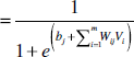
The energy function of a RBM is defined as:
where w is the weight between hidden and visible layer and b, c are biases of visible and hidden layers, respectively. V, h are visible and hidden layer nodes.
The visible and hidden layer nodes are conditionally independent.
RBM is based on probabilistic graphical models. They are ideal for unsupervised learning and can be used for unsupervised pre‐training of conventional neural networks.
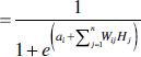
Let us assume we have V1, V2, …, VN visible nodes of N‐dimensional and H1, H2,…, HM hidden nodes of M‐dimensional. We have bias associated with each node of the hidden and visible layer. The bias associated with the visible node Vi is bi(v) and bias associated with the hidden node Hj is cj(h), and Wij is the weight associated between the visible node Vi and hidden node Hj. The RBM aims to learn weight Wij. Figure 5.3 explains the architecture of the RBM.
5.2.1.1 Training Boltzmann Machine
Training of Boltzmann machine is done through contrastive divergence (CD) [11] using Gibbs Sampling:
- The visible state is fed with the training dataset.
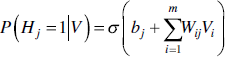
- Positive phase:
Hidden state nodes are calculated from visible nodes known as positive statistics of edge Eij which is P(Hj = 1|V). The individual activation probabilities for the hidden layer can be calculated as
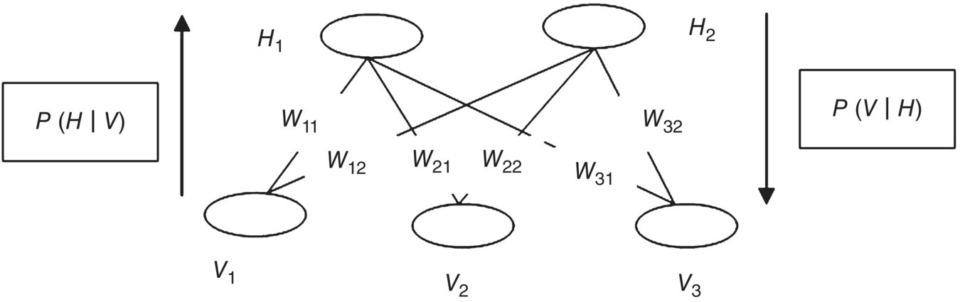
Figure 5.3 Restricted Boltzmann machine basic architecture.
- Negative phase:
In the negative phase, the input data is reconstructed using the hidden state values known as negative statistics of edge Eij, which is P(Vi = 1|H).
The individual activation probabilities for visible layer nodes can be calculated as:

- Update the weight of the edge:
The updated weight is calculated as:

and α is the learning rate.
- Repeat till the threshold is achieved.
5.2.1.2 Applications of RBM
RBM has various applications in the field of classification of data in the form of text, images, etc. It can also be used for reducing a number of variables for obtaining principle variables known as dimensionality reduction and can be used for feature selection and feature extraction. Other applications include processing of unstructured data, images, videos, collaborative filtering, topic modeling, missing value issue, etc. RBM has been applied for supervised and unsupervised learning, and an energy‐efficient RBM processor has been proposed for on‐chip learning for IoT [12]. Sourav Bhattacharya and Nicholas D. Lane [13] proposed RBM as a DL architecture for robust activity recognition using smart watches, like sleeping patterns and emotional states. They are used for predicting energy consumption in IoT.
The variants of RBMs include (i) discriminative restricted Boltzmann machine (DRBM): they are meant for the selection of parameters, which are analytical for performance. (ii) Hybrid restricted Boltzmann machine (HRBM): it includes features of both generative and discriminative models. (iii) Conditional restricted Boltzmann machine (CRBM). (iv) Robust Boltzmann machine (RoBM): it deals with eliminating noise and influence of corrupted pixels in an image.
5.2.2 Deep Belief Networks (DBN)
DBNs are one of the variants or emerging application [14] of the RBM. They form generative graphical models and are one of the solutions of vanishing gradient problem. Vanishing gradient means loss of error with respect to weights. This means when we move backward in case of backpropagation, the earlier layers of neuron are smaller as compared to the last layer. RBM has the advantage of fitting the input features, and thus hidden layer output of one layer can be used as input to a visible layer of another layer. DBNs are constructed by stacking more than one RBM. The Greedy approach is used for learning of DBNs. The number of layers stacked depends on the algorithm and thus extract features from already extracted features from the previous layer. Training the network means learning the weights. Here, training is performed in a greedy layer‐by‐layer unsupervised algorithm [15]. Hinton et al. [16] proposed fine‐tuning after training of each layer using backpropagation.
Training in DBN is divided into two phases: In the first phase, each layer has been trained using CD algorithm. The posterior probabilities p(h1 ∣ v) and p(v ∣ h1) are computed from the first layer. And then they are computed again and again till they converge as computed in the RBM. The h1 computed from visible layer after convergence is taken as v (input) for the next layer and compute h2 and same has to be propagated till last layer. In the second phase, whole DBN is fine‐tuned. Figure 5.4 explains the architecture of DBNs.
5.2.2.1 Training DBN
- Train the first layer of RBM using CD algorithm and learn the weights W1.
- Freeze the weight vector W1 of the first layer. Use the H1 (output of the first layer) from P (H1|V) as input for the next layer.
- Freeze the weights of second layer W2 that defines the second layer features. Use the H2 (output of the second layer) as input to the next layer.
- Proceed recursively for the next layers.
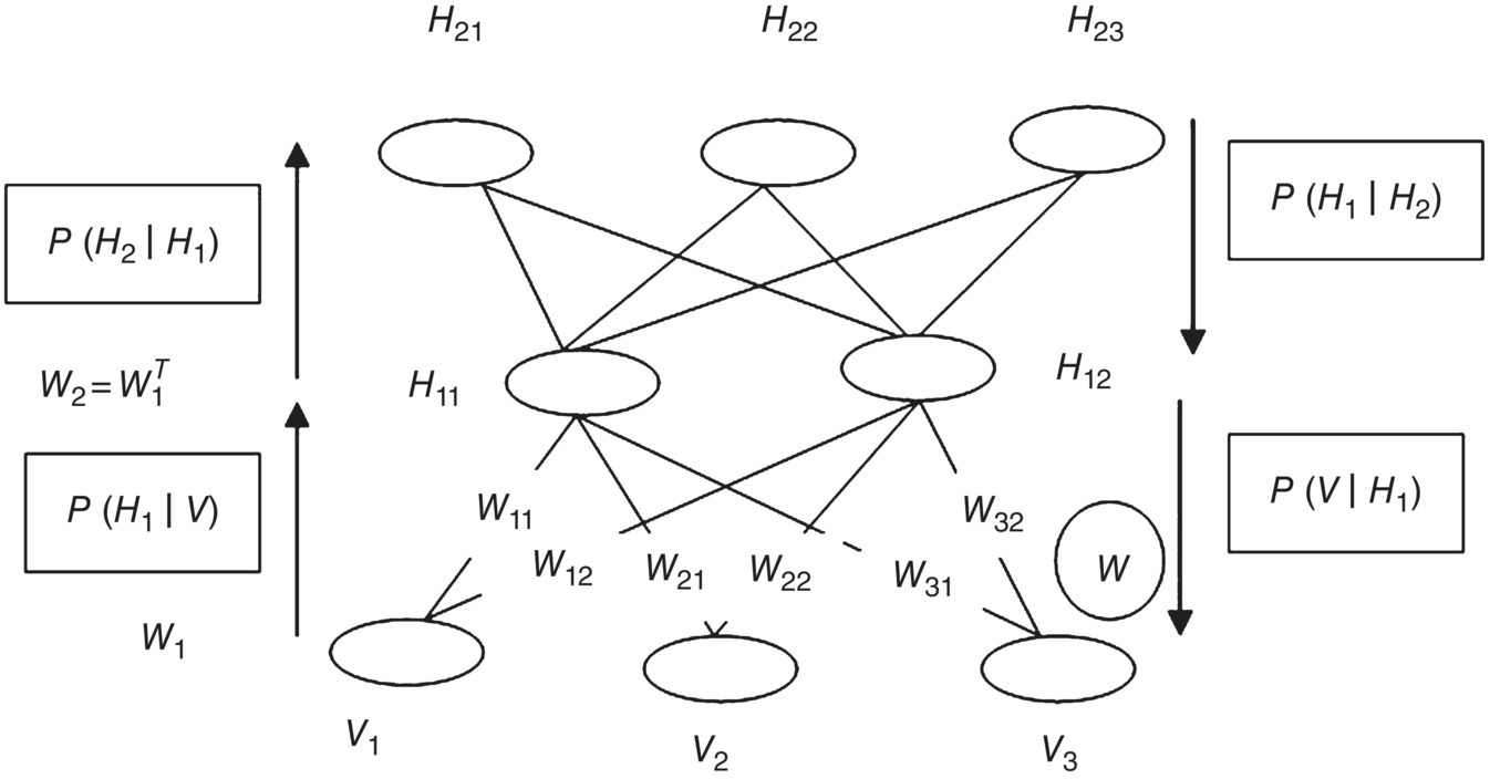
Figure 5.4 Deep belief network architecture with three layers.
5.2.2.2 Applications of DBN
It has been used to avoid overfitting and underfitting problems. It has been used for recognizing and generating images, capturing motion in a video, dimensionality reduction, audio classification, and natural language classification. They can act as feature detectors and has been applied for real‐life applications like electroencephalography [17] and drug discovery [18]. Hinton et al. [16] have deployed for the recognition and classification of handwritten characters. Ni Gao et al. [19] have deployed DBN in intrusion detection. It can provide new ideas for further research in Intrusion Detection Systems. They are suitable for hierarchical feature extraction as they use a greedy layer‐by‐layer training algorithm. It has been used for threat identification in the security and classification of faults in IoT.
5.2.3 Autoencoders
AE are unsupervised learning algorithms. They encode input in a form, from which input can be reconstructed. They convert the input into a code that is a summary of input. Thus, the size of the input is same as that of output. They are also called autoassociator. They are meant for dimensionality reduction and data compression in the areas of information processing. They extract information continuously and convert into smaller representations.
5.2.3.1 Training of AE
AE consist of three main parts: (i) encoder, (ii) code, and (iii) decoder. Figure 5.5 explains the architecture of AE. AE are self‐supervised learning algorithms because they generate their labels. The loss function measures how close the reconstructed output is to the input and is given by mean squared error:
Figure 5.5 Autoencoder architecture.
AE add a bottleneck to the network. The bottleneck forces the network to create the compress of the input. It works well if the data are correlated and does not work well if the data are not correlated.
Encoder: converts input x into some hidden representation h(x):
Decoder: reconstructs the input ![]() :
:
where b, c are biases and w is the weight vector.
w * = wT and are known as tied weights.
Variants of AE include: (i) denoising autoencoders [20]: these are the type of AE where we try to reconstruct the input from corrupted input data. They try to undo the effects of corruption in data. They improve the accuracy of OCR. (ii) Sparse autoencoder and (iii) variational autoencoder.
Variational autoencoder is a standard type of AE which shares the basic architecture of AE. Here, training is done to avoid overfitting. Encoding is done over a distribution of latent space (z). Low‐dimensional view of high‐dimensional input has been created.
5.2.3.2 Applications of AE
The applications of AE include anomaly detection, information retrieval, data denoising, etc. They are more powerful than principal component analysis (PCA). Mahmood Yousefi‐Azar et al. [21] proposed AE‐based feature learning for internet security and for various classifiers for anomaly detection in publically available datasets. Changjie Hu et al. [22] proposed improved version of AE for dimensionality reduction. It has the same number of input and output and is well suited for dimensionality reduction and feature extraction. In IoT, it can be used for emotion recognition and fault diagnosis in machinery.
5.2.4 Convolutional Neural Networks (CNN)
Convolution neural networks or ConvNet or CNN is one of the DL architecture inspired by the connectivity of neurons in human brain. It takes images (one‐dimensional or two‐dimensional or n‐dimensional) as input, converts it into smaller representation without losing information for better prediction. It consists of three primary layers: (i) convolution layer, (ii) pooling layer, and (iii) fully connected layer. Figure 5.6 explains the role of different layers of CNN architecture.

Figure 5.6 Convolution neural network architecture.
5.2.4.1 Layers of CNN
- Convolution layer: This is the main layer in a CNN. It acts as a filter to an input; when this filter is applied continuously to the input, we get feature map. Feature map gives us the locations of the important information in an image. CNN can learn filters specific to a particular training dataset. Here, multiplication is performed between input and a set of weights (called filter or kernel). The multiplication between the kernel and input is performed elementwise called dot product. The multiplication is followed by addition. Kernel size is smaller than input size; the same kernel has been applied multiple times to the different portions of an input by systematically overlapping different portions of input from left to right and top to bottom.
Whenever we are applying convolution, our output shrinks. So to avoid shrinking, we can use padding to get output dimensions the same as an input. Convolutions are of two types: (i) valid and (ii) same. In case of valid, the output we get is smaller than input and no padding is applied. In the other type, the output dimensions are the same as input, and padding is applied here. The three main parameters that control the size of output are: (i) stride, (ii) kernel size, and (iii) padding.
The step size of the filter when processing the convolution is known as a stride. The same stride size is applied both horizontally and vertically. More the stride values are smaller, the output we get. Kernel size is the filter that we apply to the input. If we want to output the same as input, then we need to include padding. CNN has the property that a part of output depends on only a smaller part of an input that is known as the sparsity of connections. A part of the image is possibly important for other parts of an image known as parameter sharing.
- Pooling layer: The function of a pooling layer is to reduce the representation size of an image. It works on feature maps extracted from the previous layer. It gives us the representation of a summary of the input, so that processing and computation are reduced. The common pooling functions include
- Max pooling: It calculates the maximum value of a portion of a feature map.
- Average pooling: It calculates the average of a portion of a feature map.
- Global pooling: This is also known as a global pooling layer. It downsamples whole feature map to a single unit.
- Fully connected layer: It is the last layer of CNN. Here, we get the class label for our input. It has a lot of connections forming a complete graph with the output from the previous layer. It gives us the decision of whole processing. Input to this layer is fed in the form of a flattened vector. At this layer, results are available.
Variants of CNN: CNN has become popular in the last few years. It has been applied to various fields and has achieved the best performance. Popular variants of CNN include (i) LeNet, (ii) AlexNet, (iii) ResNet, (iv) VGG, (v) GoogLeNet, (vi) Inception Networks, (vii) Xception, etc.
5.2.4.2 Activation Functions Used in CNN
Activation functions are nonlinear functions that decide output for the next layer. The activation functions used in CNN include:
- Sigmoid Function: It is also known as logistic activation function. It translates input (−∞, +∞) to (0, 1) used for binary class problem.
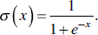
Figure 5.7 shows the graph of sigmoid function. Soft‐max logistic equation is used for multi‐class problems. This is used in the last layer of CNN.
- Tanh(): This is same as sigmoid activation function but here it translates to (−1, 1). Figure 5.8 shows a graph of Tanh() function.

- ReLU: ReLU stands for a rectified linear unit. It gives linear output for positive values and 0 for negative values. It converges faster and is used in the convolution layer of CNN in the middle layers.
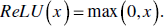
Figure 5.9 shows a graph of ReLU function. It has the problem of dying ReLU, which means if it gets 0 value, it is difficult for it to get back. Its variants include Leaky ReLU, PReLU, and ELU.
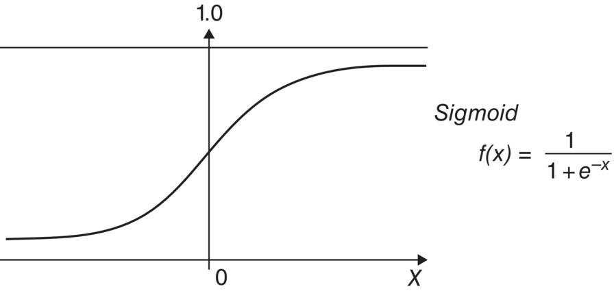
Figure 5.7 The sigmoid function.
Figure 5.8 Tanh() function.
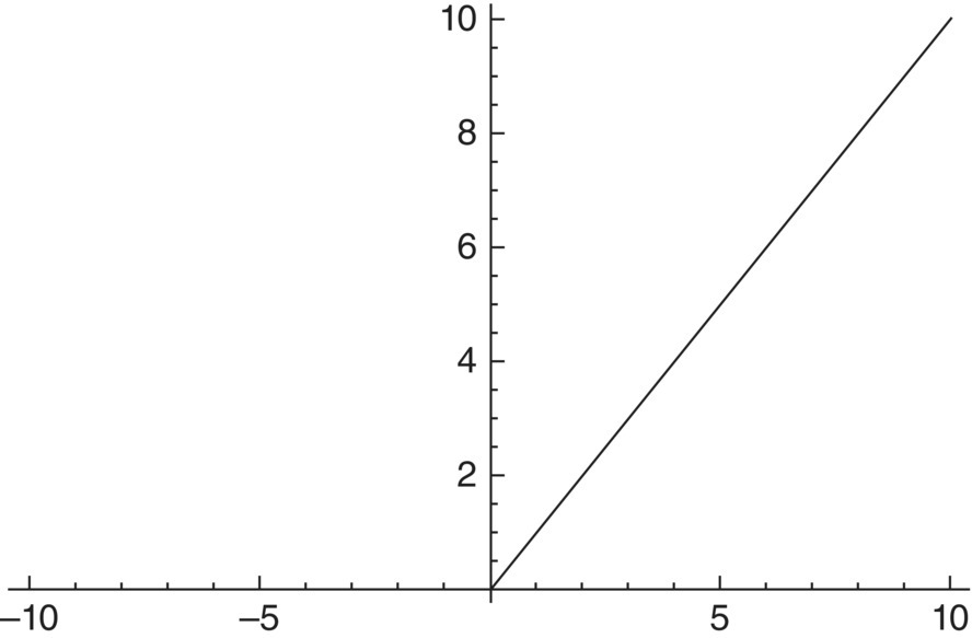
Figure 5.9 ReLU function.
5.2.4.3 Applications of CNN
CNN has proven satisfying in the field of image recognition, image transformations, face recognition, speech recognition, image labeling, recommendation system, handwriting recognition, natural language processing (NLP), behavior recognition, object recognition, etc. Iman Azimi et al. [23] have deployed CNN in the IoT healthcare system. Alberto Pacheco [24] et al. deployed it for the development of Smart Classroom and IoT Computing. A wavelet‐based CNN approach has been proposed for automated machinery fault diagnosis [25]. Parkinson's disease patients' prediction can be done using CNNs [26]. CNNs are also used for mapping sequence of ECG samples to a sequence of rhythm classes to develop high diagnostic performance similar to professionals [27]. CNNs have been used for automatic segmentation of MRI scans to predict the risk of osteoarthritis [28]. V. Gulshan et al. [27] have used CNNs to identify retinopathy. A CNN‐based approach is introduced for surface integration inspection in [29] to extract patch features and find defected areas via thresholding and segmenting. A wavelet‐based CNN approach has been proposed for automated machinery fault diagnosis [25].
5.2.5 Generative Adversarial Network (GANs)
Generative adversarial networks (GANs) are a DL architecture developed in 2014 by Ian Good Fellow. They are used for unsupervised learning and can catch and copy the dissimilarity within a dataset. They are inspiring recent discoveries in DL. GANs are generative models and build new data instances that match provided training data. They can build images that resemble images of individual faces, even though these faces do not relate to any existing person.
5.2.5.1 Training of GANs
It mainly consists of two neural network architectures that contest with one another for learning. The two networks compete with each other to generate some new probability distribution that is indistinguishable to original. GANs generate the imitate data from some original data. It consists of two main parts:
- Discriminator: The role of the discriminator module is to discriminate between original and fraud data.
- Generator: The role of the generator module is to generate the fraud data in such a way that it can deceive the discriminator. That is, data produced here must look like the original.
Figure 5.10 shows the basic framework of GANs for identifying fake or real things. Learning in GANs means deceiving the discriminator, i.e. the discriminator treats fake instances as real. The discriminator weights are kept fixed, the error is backpropagated, and weight adjustment is done at the generator. Figure 5.11 explains the basic architecture of GANs.
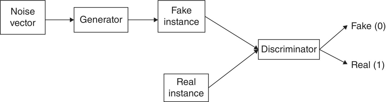
Figure 5.10 The framework of generative adversarial networks (GANs).
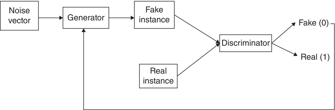
Figure 5.11 Generative adversial networks (GANs).
5.2.5.2 Variants of GANs
The variants of GANs include progressive GANs, conditional GANs, Image to Image GANs, and Cycle GANs.
5.2.5.3 Applications of GANs
GANs have been applied mainly in the field of data generation [30]. They have been successfully applied in the field of computer vision and NLP. The applications in the field of computer vision include image translation, image synthesis, and video generation. Ledig et al. [31] have applied GANs for improvement in the resolution of an image. Li and Wand [32] applied it in the field of texture synthesis. Tulyakov et al. [33] proposed GANs for video generation. They have a great opportunity to be applied in new fields and have been applied for the labeling of unlabeled images [34].
5.2.6 Recurrent Neural Networks (RNN)
CNN discussed previously is a feed‐forward neural network and can solve a lot of problems related to unstructured data. But it cannot solve a problem related to time series. To solve problems related to time series, RNN has been developed. RNNs are called recurrent because they accomplish the same task for every component of a sequence, with the output staying dependent on the early estimates. RNNs produce recorded success in many NLP tasks. The most regularly used type of RNNs is LSTMs. They are more qualified at capturing long‐term dependencies. Their applications include mainly NLP, speech recognition, handwriting recognition, etc. The nodes of RNN are directly connected to each other to form a loop‐like structure. RNNs are designed for time series input data with no fixed sized input. The data is fed in the form of series, a single data item in a series have effect from neighbor data items and affect the others in neighborhood. They have one or more input vectors and generate one or more output vectors.
5.2.6.1 Training of RNN
Training RNN is comparable to training a Neural Network. Here also backpropagation algorithm is used, but with modification. The parameters are shared by all time‐steps in the network; the gradient at each output depends on the estimates of the current time step, and previous time steps. To calculate the gradient at each point, backpropagation is needed to be called backpropagation through time (BPTT). Figure 5.12 explains the basic architecture of RNN.
The hidden state at a particular time is a function (Fw) of previous state (St−1) and current input (Xt).
where Ws, Wx are weights.
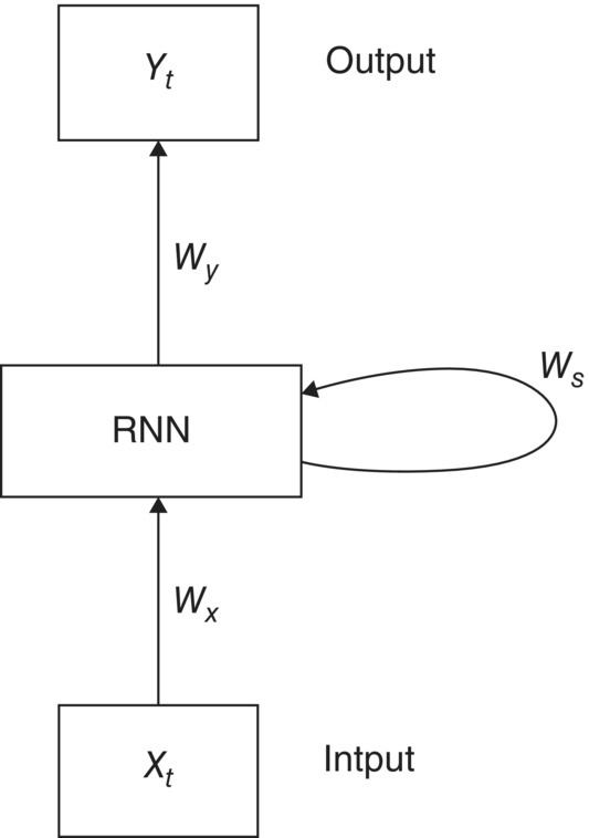
Figure 5.12 Recurrent neural network basic framework.
5.2.6.2 Applications of RNN
The RNN is trained using BPTT algorithm [35]. It is difficult to learn long‐term dependencies in the input sequence due to the decrease in error gradient as it propagates backward known as vanishing gradient problem. This leads to larger weights which in turn lead to unstable training. B. Chandra, Rajesh Kumar Sharma [36] has proposed the improved version of RNN which reduced vanishing gradient problem and has promising results for image classification. It learns complex patterns in the IoT.
5.2.7 Long Short‐Term Memory (LSTM)
LSTM is a special type of RNN proposed by German scholar Sepp Hochreiter and Juergen Schmidhuber to solve vanishing gradient problem [37]. LSTMs are a distinct kind of RNN, competent in learning long‐term dependencies and retaining information for a lengthened period of time. The LSTM model is assembled in the form of a chain structure. But, the perpetual module has a diverse arrangement. Instead of a single neural network like a standard RNN, it has four layers with a different style of communication. It stores information in the hidden layer and particularly discards information of no use in the hidden layer. Thus, it has the decision power of what to store and what to discard. It shares the basic architecture of RNN but has more compound structure inside.
5.2.7.1 Training of LSTM
LSTM consists of a chain of repeating modules called memory cells which consists of four gates. These four gates decide what information to keep or discard, handle dependencies, and handle the storage of information [38]. The four gates are:
- Input gate (i)
- Output gate (o)
- Forget gate (f)
- Memory gate (c).
The information is passed based on the weights and these weights are adjusted during the learning process. Each memory cell correlates with a time step [39]. It removes information through the forget gate, it specifically controls information transmission using the sigmoid function. Thus, outputs values between 0 and 1. One determines to keep the information and zero to discard the information. They maintain a constant error throughout; therefore, they are able to learn over multiple layers and time steps. They sustain information for a more prolonged time. Each cell has its individual decision power related to information. Forget gate removes irrelevant information, thus helps in intensification in the process. Input gate adds information, output gate selects necessary information for the output. Figure 5.13 explains the architecture of LSTM.

Figure 5.13 LSTM architecture.
5.2.7.2 Applications of LSTM
LSTM has mainly been developed for handling sequential data, NLP [40]. They have been developed for intrusion detection for learning patterns [41]. It has also been proposed for the classification of voltage dips and automatic extraction of features [42]. LSTM has become one of the most popular techniques in DL; research is going on in this field. It has been also proposed to control dynamic systems [43]. It has proven better for the classification and identification of fault with 99.80% accuracy [44]. The other applications include text generation, handwriting recognition [45], handwriting generation, music generation, language translation, and image captioning. In industries, it has been used for the analysis of equipments of IoT [46] and also for time series data generation in IoT, anomaly detection, etc. Time series data are highly complex, dynamic data, and has higher dimensionality, so it requires IoT of resources. LSTM allows forgetting unnecessary data and thus reduces the computation power needed. It can keep track of dependencies between data.
5.3 Conclusion
A thorough study of how DL carries new opportunities to the IoT has been carried out. Many IoT applications have been enabled with DL technology. DL architectures are very powerful to resolve large‐scale data analysis problems. Investigation on how to build DL models and their applications for IoT has been carried out. DL extends an innovative perspective to solve the traditional queries of IoT. Both IoT and DL have seen outburst growth of research in the last few years. DL has gained popularity in the areas of computer vision, speech recognition, NLP, video summarization, and they contribute more reliable accuracy than humans. They have already been used in IoT in data fitting. IoT is the integration of devices and various day‐to‐day applications are dependent on it. DL offers an excellent opportunity to join hardware and software, and develop real‐time applications. DL models tune themselves and make changes according to new needs and have already performed well with real‐time time‐series data. Because of its unsupervised learning nature, it has achieved great success while deployed in IoT and internet search engines. In the future, it can be incorporated into various aspects of day‐to‐day life to make our tasks easier.
References
- 1 Saleem, T.J. and Chishti, M.A. (2019) Data mining for the Internet of Things data analytics. ICDM (Posters), New York; (17 July to 21 July 2019).
- 2 Saleem, T.J. and Chishti, M.A. (2019). Data analytics in the internet of things: a survey. Scalable Computing: Practice and Experience 20: 4.
- 3 Thompson, W.L. and Talley, M.F. (2019). Deep learning for IoT communications: invited presentation. 2019 53rd Annual Conference on Information Sciences and Systems (CISS), Baltimore, MD (20–22 March 2019), 1–4.
- 4 Ma, X., Yao, T., Hu, M. et al. (2019). A survey on deep learning empowered IoT applications. IEEE Access 7: 181721–181732.
- 5 Choudhury, S. and Bhowal, A. (2015). Comparative analysis of machine learning algorithms along with classifiers for network intrusion detection. 2015 International Conference on Smart Technologies and Management for Computing, Communication, Controls, Energy and Materials (ICSTM), Chennai (6–8 May 2015).
- 6 Zhang, L., Wang, S., and Liu, B. (2017). Deep Learning for Sentiment Analysis: A Survey. National Science Foundation (NSF), and by Huawei Technologies Co. Ltd.
- 7 Kubat, M. (2017). An Introduction to Machine Learning. Cham: Springer.
- 8 Mohammed, M., Khan, M.B., and Bashier, E.B.M. (2016). Machine Learning: Algorithms and Applications. Boca Raton, FL: CRC Press.
- 9 Saleem, T.J. and Chishti, M.A. (2020). Exploring the applications of machine learning in healthcare. International Journal of Sensors, Wireless Communications and Control 10 (4): 458–472.
- 10 Salakhutdinov, R., Mnih, A., and Hinton, G. (2007). Restricted Boltzmann machines for collaborative filtering. Proceedings of the 24th International Conference on Machine Learning, Corvalis, OR (June 2007), 791–748.
- 11 O'Leary, H.M., Mayor, J.M., Poon, C.‐S., Kaufmann, W.E., and Sahin, M. (2017). Classification of respiratory disturbances in Rett syndrome patients using restricted Boltzmann machine. Engineering in Medicine and Biology Society (EMBC) 2017 39th Annual International Conference of the IEEE, Seogwipo (11–15 July 2017), 442–445.
- 12 Tsai, C., Yu, W., Wong, W.H., and Lee, C. (2017). A 41.3/26.7 pJ per neuron weight RBM processor supporting on‐chip learning/inference for IoT applications. IEEE Journal of Solid‐State Circuits 52 (10): 2601–2612.
- 13 Bhattacharya, S. and Lane, N.D. (2016). From smart to deep: robust activity recognition on smartwatches using deep learning. 2016 IEEE International Conference on Pervasive Computing and Communication Workshops (PerCom Workshops), Sydney, NSW (14–18 March 2016), 1–6.
- 14 Pan, Z., Yu, W., Yi, X. et al. (2019). Recent progress on generative adversarial networks (GANs): a survey. IEEE Access 7: 36322–36333.
- 15 Bengio, Y. (2009). Learning deep architectures for AI. Foundations and Trends in Machine Learning 2 (1): 1–27. https://doi.org/10.1561/2200000006.
- 16 Hinton, G.E., Osindero, S., and The, Y.W. (2006). A fast learning algorithm for deep belief nets. Neural Computation 18 (7): 1527–1554.
- 17 Movahedi, F., Coyle, J.L., and Sejdic, E. (2018). Deep belief networks for electroencephalography: a review of recent contributions and future outlooks. IEEE Journal of Biomedical and Health Informatics 22 (3): 642–652. https://doi.org/10.1109/jbhi.2017.2727218.
- 18 Ghasemi, P.‐S. and Mehri, f. (2018). The role of different sampling methods in improving biological activity prediction using deep belief network. Journal of Computational Chemistry 22 (3): 642–652. https://doi.org/10.1109/JBHI.2017.2727218.
- 19 Gao, N., Gao, L., Gao, Q., and Wang, H. (2014). An intrusion detection model based on deep belief networks. 2014 Second International Conference on Advanced Cloud and Big Data, Huangshan (20–22 November 2014), 247–252.
- 20 Yousefi‐Azar, M., Varadharajan, V., Hamey, L., and Tupakula, U. (2017). Autoencoder‐based feature learning for cyber security applications. 2017 International Joint Conference on Neural Networks (IJCNN), Anchorage, AK (14–19 May 2017), 3854–3861.
- 21 Hu, C., Hou, X., and Lu, Y. (2014). Improving the architecture of an autoencoder for dimension reduction. 2014 IEEE 11th Intl Conf on Ubiquitous Intelligence and Computing and 2014 IEEE 11th Intl Conf on Autonomic and Trusted Computing and 2014 IEEE 14th Intl Conf on Scalable Computing and Communications and Its Associated Workshops, Bali (9–12 December 2014), 855–858.
- 22 Vincent, P., Larochelle, H., Bengio, Y., and Manzagol, P.A. (2008). Extracting and composing robust features with denoising autoencoders. Proceedings of the 25th International Conference on Machine Learning (July 2008), 1096–1103.
- 23 Azimi, J.T.‐M., Anzanpour, A., Rahmani, A.M., Soininen, A.M., and Liljeberg, P. (2018). Empowering healthcare IoT systems with hierarchical edge‐based deep learning. 2018 IEEE/ACM International Conference on Connected Health: Applications, Systems and Engineering Technologies (CHASE), Washington, DC (26–28 September 2018), 63–68.
- 24 Pacheco, P.C., Flores, E., Trujillo, E., and Marquez, P. (2018). A smart classroom based on deep learning and osmotic IoT computing. 2018 Congreso Internacional de Innovación y Tendencias en Ingeniería (CONIITI), Bogota (3–5 October 2018), 1–5.
- 25 Wang, J., Zhuang, J., Duan, L., and Cheng, W. (2016). A multi‐scale convolution neural network for featureless fault diagnosis. Proc. Int. Symp. Flexible Autom. (ISFA), Cleveland, OH (1–3 August 2016).
- 26 Hammerla, N.Y., Halloran, S., and Plötz, T. (2016). Deep, convolutional, and recurrent models for human activity recognition using wearables. Proc. 25th Int. Joint Conf. Artif. Intell. (IJCAI) (July 2016).
- 27 Gulshan, V., Peng, L., Coram, M. et al. (2016). Development and validation of a deep learning algorithm for detection of diabetic retinopathy in retinal fundus photographs. Proceedings of the JAMA 316 (22): 2402–2410.
- 28 Prasoon, A., Petersen, K., Igel, C. et al. (2013). Deep feature learning for knee cartilage segmentation using a triplanar convolutional neural network. Proc. Int. Conf. Med. Image Comput. Comput.‐Assist. Intervent. (MICCAI), Nagoya, Japan (22–26 September 2013).
- 29 Park, J.‐K., Kwon, B.‐K., Park, J.‐H., and Kang, D.‐J. (2016). Machine learning based imaging system for surface defect inspection. International Journal of Precision Engineering and Manufacturing – Green Technology 3 (3): 303–310.
- 30 Kim, S.K., McMahon, P.L., and Olukotun, K. (2010). A large‐scale architecture for restricted Boltzmann machines. 2010 18th IEEE Annual International Symposium on Field‐Programmable Custom Computing Machines, Charlotte, NC (2–4 May 2010), 201–208.
- 31 Ledig, C. Theis, L., Huszar, F., and Caballero, J. (2017). Photo‐realistic single image super‐resolution using a generative adversarial network. Proc. IEEE Conf. Comput. Vis. Pattern Recognit. (CVPR), Honolulu, HI (21–26 July 2017), 105–114.
- 32 Li, C. and Wand, M. (2016). Precomputed real‐time texture synthesis with markovian generative adversarial networks. In: Computer Vision – ECCV 2016. ECCV 2016, Lecture Notes in Computer Science, vol. 9907 (eds. B. Leibe, J. Matas, N. Sebe and M. Welling). Cham: Springer https://doi.org/10.1007/978‐3‐319‐46487‐9_43.
- 33 Huang, R., Zhang, S., Li, T., and He, R. (2017). Beyond face rotation: global and local perception GAN for photorealistic and identity preserving frontal view synthesis. Proc. IEEE Int. Conf. Comput. Vis. (ICCV), Venice, Italy (22–29 October 2017), 2439–2448.
- 34 Zhang, X.‐Y., Yin, F., Zhang, Y.‐M. et al. (2018). Drawing and recognizing Chinese characters with recurrent neural network. IEEE Transactions on Pattern Analysis & Machine Intelligence 40 (4): 849–862.
- 35 Rumelhart, D.E., Hinton, G.E., and Williams, R.J. (1986). Learning representations by back‐propagating errors. Nature 323 (6088): 533–536. https://doi.org/10.1038/323533a0. [Online].
- 36 Chandra, B. and Sharma, R.K. (2017). On improving recurrent neural network for image classification. 2017 International Joint Conference on Neural Networks (IJCNN), Anchorage, AK, Anchorage, AK, (14–19 May 2017), 1904–1907.
- 37 Hochreiter, S. and Schmidhuber, J. (1997). Long short‐term memory. Neural Computation 9 (8): 1735–1780.
- 38 Lyu, Q. and Zhu, J. (2014). Revisit long short‐term memory: an optimization perspective. In Advances in Neural Information Processing Systems Workshop on Deep Learning and Representation Learning (December 2014), pp. 1–9.
- 39 Anani, W. and Samarabandu, J. (2018). Comparison of recurrent neural network algorithms for intrusion detection based on predicting packet sequences. 2018 IEEE Canadian Conference on Electrical & Computer Engineering (CCECE), Quebec City, QC (13–16 May 2018), 1–4.
- 40 Cho, K., Van Merrienboer, B., Gulcehre, C. et al. (2014). Learning Phrase Representations Using RNN Encoder‐Decoder for Statistical Machine Translation (June 2014).
- 41 Tuor, A., Kaplan, S., Hutchinson, B. et al. (2017). Deep learning for unsupervised insider threat detection in structured cybersecurity data streams. arXiv preprint, arXiv:1710.00811.
- 42 Balouji, E., Gu, I.Y.H., Bollen, M.H.J., Bagheri, A., and Nazari, M. (2018). A LSTM‐based deep learning method with application to voltage dip classification. 2018 18th International Conference on Harmonics and Quality of Power (ICHQP), Ljubljana (13–16 May 2018), 1–5.
- 43 Wang, Y. (2017). A new concept using LSTM Neural Networks for dynamic system identification. 2017 American Control Conference (ACC), Seattle, WA (24–26 May 2017), 5324–5329.
- 44 Wang, W., Qiu, X., Chen, C., Lin, B., and Zhang, H. (2018). Application research on long short‐term memory network in fault diagnosis. 2018 International Conference on Machine Learning and Cybernetics (ICMLC), Chengdu (15–18 July 2018), 360–365.
- 45 Creswell, T., White, V., Dumoulin, K. et al. (2018). Generative adversarial networks: an overview. IEEE Signal Processing Magazine 35 (1): 53–65.
- 46 Zhang, W., Guo, W., Liu, X. et al. (2018). LSTM‐based Analysis of Industrial IoT Equipment. IEEE Access 6: 1. https://doi.org/10.1109/ACCESS.2018.2825538.