12.1 INTRODUCTION

We live in a period characterized by rapid advances in artificial intelligence (AI) and machine learning, which are transforming everyday life in amazing ways. AlphaGo Zero (Silver et al. 2017) showed that superhuman performance can be achieved by pure reinforcement learning, with only very minimal domain knowledge and (amazingly!) no reliance on human data or guidance. AlphaGo Zero learned to play after merely being told the rules of the game, and playing against a simulator (itself, in that case).

The game of Go has many aspects in common with trading. Good traders often use complex strategy and plan several periods ahead. They sometimes make decisions which are ‘long‐term greedy’ and pay the cost of a short‐term temporary loss in order to implement their long‐term plan. In each instant, there is a relatively small, discrete set of actions that the agent can take. In games such as Go and chess, the available actions are dictated by the rules of the game.

In trading, there are also rules of the game. Currently the most widely used trading mechanism in financial markets is the ‘continuous double auction electronic order book with time priority’. With this mechanism, quote arrival and transactions are continuous in time and execution priority is assigned based on the price of quotes and their arrival order. When a buy (respectively, sell) order x is submitted, the exchange's matching engine checks whether it is possible to match x to some other previously submitted sell (respectively, buy) order. If so, the matching occurs immediately. If not, x becomes active and it remains active until either it becomes matched to another incoming sell (respectively, buy) order or it is cancelled. The set of all active orders at a given price level is a FIFO queue. There's much more to say about microstructure theory and we refer to the book by Hasbrouck (2007), but these are, in a nutshell, the ‘rules of the game’.

These observations suggest the inception of a new subfield of quantitative finance: reinforcement learning for trading (Ritter 2017). Perhaps the most fundamental question in this burgeoning new field is the following.

FUNDAMENTAL QUESTION 1

Can an artificial intelligence discover an optimal dynamic trading strategy (with transaction costs) without being told what kind of strategy to look for?

If it existed, this would be the financial analogue of AlphaGo Zero.

In this note, we treat the various elements of this question:

1. What is an optimal dynamic trading strategy? How do we calculate its costs?
2. Which learning methods have even a chance at attacking such a difficult problem?
3. How can we engineer the reward function so that an AI has the potential to learn to optimize the right thing?

The first of these sub‐problems is perhaps the easiest. In finance, optimal means that the strategy optimizes expected utility of final wealth (utility is a subtle concept and will be explained below). Final wealth is the sum of initial wealth plus a number of wealth increments over shorter time periods:

(12.1)

where δw_t = w_t − w_t−1. Costs include market impact, crossing the bid‐offer spread, commissions, borrow costs, etc. These costs generally induce a negative drag on w_T because each δw_t is reduced by the cost paid in that period.

We now discuss the second question: which learning methods have a chance of working? When a child tries to ride a bicycle (without training wheels) for the first time, the child cannot perfectly know the exact sequence of actions (pedal, turn handlebars, lean left or right, etc.) that will result in the bicycle remaining balanced and going forward. There is a trial and error process in which the correct actions are rewarded; incorrect actions incur a penalty. One needs a coherent mathematical framework which promises to mimic or capture this aspect of how sentient beings learn.

Moreover, sophisticated agents/actors/beings are capable of complex strategic planning. This usually involves thinking several periods ahead and perhaps taking a small loss to achieve a greater anticipated gain in subsequent periods. An obvious example is losing a pawn in chess as part of a multi‐part strategy to capture the opponent's queen. How do we teach machines to ‘think strategically’?

Many intelligent actions are deemed ‘intelligent’ precisely because they are optimal interactions with an environment. An algorithm plays a computer game intelligently if it can optimize the score. A robot navigates intelligently if it finds a shortest path with no collisions: minimizing a function which entails path length with a large negative penalty for collision.

Learning, in this context, is learning how to choose actions wisely to optimize your interaction with your environment, in such a way as to maximize rewards received over time. Within artificial intelligence, the subfield dedicated to the study of this kind of learning is called reinforcement learning. Most of its key developments are summarized in Sutton and Barto (2018).

An oft‐quoted adage is that there are essentially three types of machine learning: supervised, unsupervised and reinforcement. As the story goes, supervised learning is learning from a labelled set of examples called a ‘training set’ while unsupervised learning is finding structure hidden in collections of unlabelled data, and reinforcement learning is something else entirely. The reality is that these forms of learning are all interconnected. Most production‐quality reinforcement learning systems employ elements of supervised and unsupervised learning as part of the representation of the value function. Reinforcement learning is about maximizing cumulative reward over time, not about finding hidden structure, but it is often the case that the best way to maximize the reward signal is by finding hidden structure.

12.2 MARKOV DECISION PROCESSES: A GENERAL FRAMEWORK FOR DECISION MAKING

Sutton and Barto (1998) say:

The key idea of reinforcement learning generally, is the use of value functions to organize and structure the search for good policies.

The foundational treatise on value functions was written by Bellman (1957), at a time when the phrase ‘machine learning’ was not in common usage. Nonetheless, reinforcement learning owes its existence, in part, to Richard Bellman.

A value function is a mathematical expectation in a certain probability space. The underlying probability measure is the one associated to a system which is very familiar to classically trained statisticians: a Markov process. When the Markov process describes the state of a system, it is sometimes called a state‐space model. When, on top of a Markov process, you have the possibility of choosing a decision (or action) from a menu of available possibilities (the ‘action space’), with some reward metric that tells you how good your choices were, then it is called a Markov decision process (MDP).

In a Markov decision process, once we observe the current state of the system, we have the information we need to make a decision. In other words (assuming we know the current state), then it would not help us (i.e. we could not make a better decision) to also know the full history of past states which led to the current state. This history‐dependence is closely related to Bellman's principle.

Bellman (1957) writes: ‘In each process, the functional equation governing the process was obtained by an application of the following intuitive.’

An optimal policy has the property that whatever the initial state and initial decision are, the remaining decisions must constitute an optimal policy with regard to the state resulting from the first decision.

Bellman (1957)

The ‘functional equations’ that Bellman is talking about are essentially (12.7) and (12.8), as we explain in the next section. Consider an interacting system: agent interacts with environment. The ‘environment’ is the part of the system outside of the agent's direct control. At each time‐step t, the agent observes the current state of the environment S_t ∈ S and chooses an action A_t ∈ A. This choice influences both the transition to the next state and the reward the agent receives (Figure 12.1).

Underlying everything, there is assumed to be a distribution

for the joint probability of transitioning to state s⁰ ∈ S and receiving reward r, conditional on the previous state being s and the agent taking action a. This distribution is typically not known to the agent, but its existence gives mathematical meaning to notions such as ‘expected reward’.

The agent's goal is to maximize the expected cumulative reward, denoted by

(12.2)

where 0 < γ < 1 is necessary for the infinite sum to be defined.

A policy π is, roughly, an algorithm for choosing the next action, based on the state you are in. More formally, a policy is a mapping from states to probability distributions over the action space. If the agent is following policy π, then in state s, the agent will choose action a with probability π(a|s).

Reinforcement learning is the search for policies which maximize

Normally, the policy space is too large to allow brute‐force search, so the search for policies possessing good properties must proceed by the use of value functions.

The state‐value function for policy π is defined to be

where Eπ denotes the expectation under the assumption that policy π is followed. For any policy π and any state s, the following consistency condition holds:

(12.3)

(12.4)

(12.5)

(12.6)

The end result of the above calculation,

is called the Bellman equation. The value function v_π is the unique solution to its Bellman equation. Similarly, the action‐value function expresses the value of starting in state s, taking action a, and then following policy π thereafter:

Policy π is defined to be at least as good as π⁰ if

for all states s.

An optimal policy is defined to be one which is at least as good as any other policy. There need not be a unique optimal policy, but all optimal policies share the same optimal state‐value function

and optimal action‐value function

Note that v_*(s) = max_a q_*(s,a), so the action‐value function is more general than the state‐value function.

The optimal state‐value function and action‐value function satisfy the Bellman equations

(12.7)

(12.8)

where the sum over s⁰,r denotes a sum over all states s⁰ and all rewards r.

If we possess a function q(s,a) which is an estimate of q_*(s,a), then the greedy policy (associated to the function q) is defined as picking at time t the action which maximizes q(s_t,a) over all possible a, where s_t is the state at time t. Given the function q_*, the associated greedy policy is the optimal policy. Hence we can reduce the problem to finding q_*, or producing a sequence of iterates that converges to q_*.

It is worth noting at this point that modern approaches to multi‐period portfolio optimization with transaction costs (Gârleanu and Pedersen 2013; Kolm and Ritter 2015; Benveniste and Ritter 2017) are also organized as optimal control problems which, in principle, could be approached by finding solutions to (12.7), although these equations are difficult to solve with constraints and non‐differentiable costs.

There is a simple algorithm which produces a sequence of functions converging to q_*, known as Q‐learning (Watkins 1989). Many subsequent advancements built upon Watkins' seminal work, and the original form of Q‐learning is perhaps no longer the state of the art. Among its drawbacks include that it can require a large number of time‐steps for convergence.

The Watkins algorithm consists of the following steps. One initializes a matrix Q with one row per state and one column per action. This matrix can be initially the zero matrix, or initialized with some prior information if available. Let S denote the current state.

Repeat the following steps until a pre‐selected convergence criterion is obtained:

1. Choose action A ∈ A using a policy derived from Q which combines exploration and exploitation.
2. Take action A, after which the new state of the environment is S⁰ and we observe reward R.
3. Update the value of Q(S,A): set.

and

(12.9)

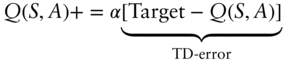
where α ∈ (0,1) is called the step‐size parameter. The step‐size parameter does not have to be constant and indeed can vary with each time‐step. Convergence proofs usually require this; presumably the MDP generating the rewards has some unavoidable process noise which cannot be removed with better learning, and thus the variance of the TD‐error never goes to zero. Hence α_t must go to zero for large time‐step t.

Assuming that all state‐action pairs continue to be updated, and assuming a variant of the usual stochastic approximation conditions on the sequence of step‐size parameters (see (12.10) below), the Q‐learning algorithm has been shown to converge with probability 1 to q_*.

In many problems of interest, either the state space, or the action space, or both are most naturally modelled as continuous spaces (i.e. sub‐spaces of R^d for some appropriate dimension d). In such a case, one cannot directly use the algorithm above. Moreover, the convergence result stated above does not generalize in any obvious way.

Many recent studies (for example, Mnih et al. (2015)) have proposed replacing the Q‐matrix in the above algorithm with a deep neural network. Unlike a lookup table, a neural network has a vector of associated parameters, sometimes called weights. We could then write the Q‐function as Q(s,a;θ), emphasizing its parameter dependence. Instead of iteratively updating values in a table, we will iteratively update the parameters, θ, so that the network learns to compute better estimates of state‐action values.

Although neural networks are general function approximators, depending on the structure of the truly‐optimal Q‐function q_*, it may be the case that a neural network learns very slowly, both in terms of the CPU time needed to train and also in terms of efficient sample use (defined as a lower number of samples required to achieve acceptable results). The network topology and the various choices such as activation functions and optimizer (Kingma and Ba 2014) matter quite a bit in terms of training time and efficient sample use.

In some problems, the use of simpler function‐approximators (such as ensembles of regression trees) to represent the unknown function Q(s,a;θ) may lead to much faster training time and much more efficient sample use. This is especially true when q_* can be well approximated by a simple functional form such as a locally linear form.

The observant reader will have noticed the similarity of the Q‐learning update procedure to stochastic gradient descent. This fruitful connection was noted and exploited by Baird III and Moore (1999), who reformulate several different learning procedures as special cases of stochastic gradient descent.

The convergence of stochastic gradient descent has been studied extensively in the stochastic approximation literature (Bottou 2012). Convergence results typically require learning rates satisfying the conditions

(12.10)

The theorem of Robbins and Siegmund (1985) provides a means to establish almost sure convergence of stochastic gradient descent under surprisingly mild conditions, including cases where the loss function is non‐smooth.

12.3 RATIONALITY AND DECISION MAKING UNDER UNCERTAINTY

Given some set of mutually exclusive outcomes (each of which presumably affects wealth or consumption somehow), a lottery is a probability distribution on these events such that the total probability is 1. Often, but not always, these outcomes involve gain or loss of wealth. For example, ‘pay 1000 for a 20% chance to win 10,000’ is a lottery.

Nicolas Bernoulli described the St Petersburg lottery/paradox in a letter to Pierre Raymond de Montmort on 9 September 1713. A casino offers a game of chance for a single player in which a fair coin is tossed at each stage. The pot starts at $2 and is doubled every time a head appears. The first time a tail appears, the game ends and the player wins whatever is in the pot. The mathematical expectation value is

This paradox led to a remarkable number of new developments as mathematicians and economists struggled to understand all the ways it could be resolved.

Daniel Bernoulli (cousin of Nicolas) in 1738 published a seminal treatise in the Commentaries of the Imperial Academy of Science of Saint Petersburg; this is, in fact, where the modern name of this paradox originates. Bernoulli's work possesses a modern translation (Bernoulli 1954) and thus may be appreciated by the English‐speaking world.

The determination of the value of an item must not be based on the price, but rather on the utility it yields… There is no doubt that a gain of one thousand ducats is more significant to the pauper than to a rich man though both gain the same amount.

Bernoulli (1954)

Among other things, Bernoulli's paper contains a proposed resolution to the paradox: if investors have a logarithmic utility, then their expected change in utility of wealth by playing the game is finite.

Of course, if our only goal were to study the St Petersburg paradox, then there are other, more practical resolutions. In the St Petersburg lottery only very unlikely events yield the high prizes that lead to an infinite expected value, so the expected value becomes finite if we are willing to, as a practical matter, disregard events which are expected to occur less than once in the entire lifetime of the universe.

Moreover, the expected value of the lottery, even when played against a casino with the largest resources realistically conceivable, is quite modest. If the total resources (or total maximum jackpot) of the casino are W dollars, then L = blog₂(W)c is the maximum number of times the casino can play before it no longer fully covers the next bet, i.e. 2^L ≤ W but 2^L+1 > W. The mutually exclusive events are that you flip one time, two times, three times, …, L times, winning 2¹,2²,2³,…,2^L or finally, you flip 2^L+1 times and win W. The expected value of the lottery then becomes:

If the casino has W = $1 billion, the expected value of the ‘realistic St Petersburg lottery’ is only about $30.86.

If lottery M is preferred over lottery L, we write L ≺ M. If M is either preferred over or viewed with indifference relative to L, we write . If the agent is indifferent between L and M, we write L ∼ M. Von Neumann and Morgenstern (1945) provided the definition of when the preference relation is rational, and proved the key result that any rational preference relation has an expression in terms of a utility function.

12.4 MEAN‐VARIANCE EQUIVALENCE

In the previous section we recalled the well‐known result that for an exponential utility function and for normally distributed wealth increments, one may dispense with maximizing E[u(w_T)] and equivalently solve the mathematically simpler problem of maximizing E[w_T] − (κ/2)V[w_T]. Since this is actually the problem our reinforcement learning systems are going to solve, naturally we'd like to know the class of problems to which it applies. It turns out that neither of the conditions of normality or exponential utility is necessary; both can be relaxed very substantially.

The k‐th central moment of x will be

From this it is clear that all odd moments will be zero and the 2k‐th moment will be proportional to ω^2k. Therefore the full distribution of x is completely determined by μ,ω, so expected utility is a function of μ,ω.

We now prove the inequalities (12.19). Write

(12.20)

Note that the integral is over a one‐dimensional variable. Using the special case of Eq. (12.16) with n = 1, we have

(12.21)

Using (12.21) to update (12.20), we have

Now make the change of variables z = (x − μ)/ω and dx = ω dz, which yields

The desired property ≥ 0 then follows immediately from the condition from Definition 2 that u is increasing.

The case for goes as follows:

A differentiable function is concave on an interval if and only if its derivative is monotonically decreasing on that interval, hence

while g₁(z²) > 0 since it is a probability density function. Hence on the domain of integration, the integrand of is non‐positive and hence ≤ 0, completing the proof of Theorem 2.

Recall Definition 5 above of indifference curves. Imagine the indifference curves written in the σ,μ plane with σ on the horizontal axis. If there are two branches of the curve, take only the upper one. Under the conditions of Theorem 2, one can make two statements about the indifference curves:

• dμ/dσ > 0 or an investor is indifferent about two portfolios with different variances only if the portfolio with greater σ also has greater μ,
• d²μ/dσ² > 0, or the rate at which an individual must be compensated for accepting greater σ (this rate is dμ/dσ) increases as σ increases

These two properties say that the indifference curves are convex.

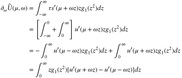
In case you are wondering how one might calculate dμ/dσ along an indifference curve, we may assume that the indifference curve is parameterized by

and differentiate both sides of

with respect to λ. By assumption, the left side is constant (has zero derivative) on an indifference curve. Hence

If u⁰ > 0 and u⁰⁰ < 0 at all points, then the numerator ^RR z u⁰(μ + σz)g₁(z²)dz is negative, and so dμ/dσ > 0.

The proof that d²μ/dσ² > 0 is similar (exercise).

What, exactly, fails if the distribution p(r) is not elliptical? The crucial step of this proof assumes that a two‐parameter distribution f(x;μ,σ) can be put into ‘standard form’ f(z;0,1) by a change of variables z = (x − μ)/σ. This is not a property of all two‐parameter probability distributions; for example, it fails for the lognormal.

One can see by direct calculation that for logarithmic utility, u(x) = logx and for a log‐normal distribution of wealth,

then the indifference curves are not convex. The moments of x are

and with a little algebra one has

One may then calculate dμ/dσ and d²μ/dσ² along a parametric curve of the form

and see that dμ/dσ > 0 everywhere along the curve, but d²μ/dσ² changes sign. Hence this example cannot be mean‐variance equivalent.

Theorem 2 implies that for a given level of median return, the right kind of investors always dislike dispersion. We henceforth assume, unless otherwise stated, that the first two moments of the distribution exist. In this case (for elliptical distributions), the median is the mean and the dispersion is the variance, and hence the underlying asset return distribution is mean‐variance equivalent in the sense of Definition 4. We emphasize that this holds for any smooth, concave utility.

12.5 REWARDS

In some cases the shape of the reward function is not obvious. It's part of the art of formulating the problem and the model. My advice in formulating the reward function is to think very carefully about what defines ‘success’ for the problem at hand, and in a very complete way. A reinforcement learning agent can learn to maximize only the rewards it knows about. If some part of what defines success is missing from the reward function, then the agent you are training will most likely fall behind in exactly that aspect of success.

12.5.1 The form of the reward function for trading

In finance, as in certain other fields, the problem of reward function is also subtle, but happily this subtle problem has been solved for us by Bernoulli (1954), Von Neumann and Morgenstern (1945), Arrow (1971) and Pratt (1964). The theory of decision making under uncertainty is sufficiently general to encompass very many, if not all, portfolio selection and optimal‐trading problems; should you choose to ignore it, you do so at your own peril.

Consider again maximizing (12.12):

(12.22)

Suppose we could invent some definition of ‘reward’ R_t so that

(12.23)

Then (12.22) looks like a ‘cumulative reward over time’ problem.

Reinforcement learning is the search for policies which maximize

which by (12.23) would then maximize expected utility as long as γ ≈ 1.

Consider the reward function

(12.24)

where is an estimate of a parameter representing the mean wealth increment over one period, μ = E[δw_t].

Then and for large T, the two terms on the right‐hand side approach the sample mean and the sample variance, respectively.

Thus, with this one special choice of the reward function (12.24), if the agent learns to maximize cumulative reward, it should also approximately maximize the meanvariance form of utility.

12.5.2 Accounting for profit and loss

Suppose that trading in a market with N assets occurs at discrete times t = 0,1,2,…,T. Let n_t ∈ Z^N denote the holdings vector in shares at time t, so that

denotes the vector of holdings in dollars, where p_t denotes the vector of midpoint prices at time t.

Assume for each t, a quantity δn_t shares are traded in the instant just before t and no further trading occurs until the instant before t + 1. Let

denote the ‘portfolio value’, which we define to be net asset value in risky assets, plus cash. The profit and loss (PL) before commissions and financing over the interval [t,t + 1) is given by the change in portfolio value δv_{t + 1}.

For example, suppose we purchase δn_t = 100 shares of stock just before t at a per‐share price of p_t = 100 dollars. Then nav_t increases by 10 000 while cash_t decreases by 10 000, leaving v_t invariant. Suppose that just before t + 1, no further trades have occurred and p_t+1 = 105; then δv_t+1 = 500, although this PL is said to be unrealized until we trade again and move the profit into the cash term, at which point it is realized.

Now suppose p_t = 100 but due to bid‐offer spread, temporary impact or other related frictions our effective purchase price was . Suppose further that we continue to use the midpoint price p_t to ‘mark to market’, or compute net asset value. Then, as a result of the trade, nav_t increases by (δn_t)p_t = 10 000 while cash_t decreases by 10 100, which means that v_t is decreased by 100 even though the reference price p_t has not changed. This difference is called slippage; it shows up as a cost term in the cash part of v_t.

Executing the trade list results in a change in cash balance given by

where is our effective trade price including slippage. If the components of δn_t were all positive then this would represent payment of a positive amount of cash, whereas if the components of δn_t were negative we receive cash proceeds.

Hence before financing and borrow cost, one has

(12.25)

(12.26)

(12.27)

(12.28)

where the asset returns are r_t = p_t/p_t−1 − 1. Let us define the total cost c_t inclusive of both slippage and borrow/financing cost as follows:

(12.29)

(12.30)

where fin_t denotes the commissions and financing costs incurred over the period, commissions are proportional to δn_t and financing costs are convex functions of the components of n_t. The component slip_t is called the slippage cost. Our conventions are such that fin_t > 0 always, and slip_t > 0 with high probability due to market impact and bid‐offer spreads.

12.6 PORTFOLIO VALUE VERSUS WEALTH

Combining (12.29),(12.30) with (12.28) we have finally

(12.31)

If we could liquidate the portfolio at the midpoint price vector p_t, then v_t would represent the total wealth at time t associated to the trading strategy under consideration. Due to slippage it is unreasonable to expect that a portfolio can be liquidated at prices p_t, which gives rise to costs of the form (12.30).

Concretely, v_t = nav_t + cash_t has a cash portion and a non‐cash portion. The cash portion is already in units of wealth, while the non‐cash portion nav_t = n_t ·p_t could be converted to cash if a cost were paid; that cost is known as liquidation slippage:

Hence it is the formula for slippage, but with δn_t = −n_t. Note that liquidation is relevant at most once per episode, meaning the liquidation slippage should be charged at most once, after the final time T.

To summarize, we may identify v_t with the wealth process w_t as long as we are willing to add a single term of the form

(12.32)

to the multi‐period objective. If T is large and the strategy is profitable, or if the portfolio is small compared with the typical daily trading volume, then liqslip _T ≪ v_T and (12.32) can be neglected without much influence on the resulting policy. In what follows, for simplicity we identify v_t with total wealth w_t.

12.7 A DETAILED EXAMPLE

Formulating an intelligent behaviour as a reinforcement learning problem begins with identification of the state space S and the action space A. The state variable s_t is a data structure which, simply put, must contain everything the agent needs to make a trading decision, and nothing else. The values of any alpha forecasts or trading signals must be part of the state, because if they aren't, the agent can't use them.

Variables that are good candidates to include in the state:

1. The current position or holding.
2. The values of any signals which are believed to be predictive.
3. The current state of the market microstructure (i.e. the limit order book), so that the agent may decide how best to execute.

In trading problems, the most obvious choice for an action is the number of shares to trade, δn_t, with sell orders corresponding to δn_t < 0. In some markets there is an advantage to trading round lots, which constrains the possible actions to a coarser lattice. If the agent's interaction with the market microstructure is important, there will typically be more choices to make, and hence a larger action space. For example, the agent could decide which execution algorithm to use, whether to cross the spread or be passive, target participation rate, etc.

We now discuss how the reward is observed during the trading process. Immediately before time t, the agent observes the state p_t and decides an action, which is a trade list δn_t in units of shares. The agent submits this trade list to an execution system and then can do nothing until just before t + 1.

The agent waits one period and observes the reward

(12.33)

The goal of reinforcement learning in this context is that the agent will learn how to maximize the cumulative reward, i.e. the sum of (12.33) which approximates the mean‐variance form E[δv] − (κ/2)V[δv].

For this example, assume that there exists a tradable security with a strictly positive price process p_t > 0. (This ‘security’ could itself be a portfolio of other securities, such as an ETF or a hedged relative‐value trade.)

Further suppose that there is some ‘equilibrium price’ p_e such that x_t = log(p_t/p_e) has dynamics

(12.34)

where ξ_t ∼ N(0,1) and ξ_t,ξ_s are independent when t 6 = s. This means that p_t tends to revert to its long‐run equilibrium level p_e with mean‐reversion rate λ. These assumptions imply something similar to an arbitrage! Positions taken in the appropriate direction while very far from equilibrium have very small probability of loss and extremely asymmetric loss‐gain profiles.

For this exercise, the parameters of the dynamics (12.34) were taken to be λ = log(2)/H, where H = 5 is the half‐life, σ = 0.1 and the equilibrium price is p_e = 50.

All realistic trading systems have limits which bound their behaviour. For this example we use a reduced space of actions, in which the trade size δn_t in a single interval is limited to at most K round lots, where a ‘round lot’ is usually 100 shares (most institutional equity trades are in integer multiples of round lots). Also we assume a maximum position size of M round lots. Consequently, the space of possible trades, and also the action space, is

Letting H denote the possible values for the holding n_t, then similarly

For the examples below, we take K = 5 and M = 10.

Another feature of real markets is the tick size, defined as a small price increment (such as US$0.01) such that all quoted prices (i.e. all bids and offers) are integer multiples of the tick size. Tick sizes exist in order to balance price priority and time priority. This is convenient for us since we want to construct a discrete model anyway. We use TickSize = 0.1 for our example.

We choose boundaries of the (finite) space of possible prices so that sample paths of the process (12.34) exit the space with vanishingly small probability. With the parameters as above, the probability that the price path ever exits the region [0.1, 100] is small enough that no aspect of the problem depends on these bounds.

Concretely, the space of possible prices is:

We do not allow the agent, initially, to know anything about the dynamics. Hence, the agent does not know λ,σ, or even that some dynamics of the form (12.34) are valid. The agent also does not know the trading cost. We charge a spread cost of one tick size for any trade. If the bid‐offer spread were equal to two ticks, then this fixed cost would correspond to the slippage incurred by an aggressive fill which crosses the spread to execute. If the spread is only one tick, then our choice is overly conservative. Hence

(12.35)

We also assume that there is permanent price impact which has a linear functional form: each round lot traded is assumed to move the price one tick, hence leading to a dollar cost |δn_t| × TickSize/LotSize per share traded, for a total dollar cost for all shares

(12.36)

The total cost is the sum

Our claim is not that these are the exact cost functions for the world we live in, although the functional form does make some sense.

The state of the environment s_t = (p_t,n_{t − 1}) will contain the security prices p_t, and the agent's position, in shares, coming into the period: n_{t − 1}. Therefore the state space is the Cartesian product S = H × P. The agent then chooses an action

which changes the position to n_t = n_t−1 + δn_t and observes a profit/loss equal to

and a reward

as in Eq. (12.33).

We train the Q‐learner by repeatedly applying the update procedure involving (12.9). The system has various parameters which control the learning rate, discount rate, risk aversion, etc. For completeness, the parameter values used in the following example were: We use n_train = 10⁷ training steps (each ‘training step’ consists of one action‐value update as per (12.9)) and then evaluate the system on 5000 new samples of the stochastic process (see Figure 12.2).

The excellent performance out‐of‐sample should perhaps be expected; the assumption of an Ornstein‐Uhlenbeck process implies a near arbitrage in the system. When the price is too far out of equilibrium, a trade betting that it returns to equilibrium has a very small probability of a loss. With our parameter settings, even after costs this is true. Hence the existence of an arbitrage‐like trading strategy in this idealized world is not surprising, and perfect mean‐reverting processes such as (12.34) need not exist in real markets.

Rather, the surprising point is that the Q‐learner does not, at least initially, know that there is mean‐reversion in asset prices, nor does it know anything about the cost of trading. At no point does it compute estimates for the parameters λ,σ. It learns to maximize expected utility in a model‐free context, i.e. directly from rewards rather than indirectly (using a model).

We have also verified that expected utility maximization achieves a much higher out‐of‐sample Sharpe ratio than expected‐profit maximization. Understanding of this principle dates back at least to 1713 when Bernoulli pointed out that a wealth‐maximizing investor behaves nonsensically when faced with gambling based on a martingale (see Bernoulli (1954) for a recent translation).

12.8 CONCLUSIONS AND FURTHER WORK

In the present chapter, we have seen that reinforcement learning concerns the search for good value functions (and hence, good policies). In almost every subfield of finance, this kind of model of optimal behaviour is fundamental. For examples, most of the classic works on market microstructure theory (Glosten and Milgrom 1985; Copeland and Galai 1983; Kyle 1985) model both the dealer and the informed trader as optimizing their cumulative monetary reward over time. In many cases the cited authors assume the dealer simply trades to maximize expected profit (i.e. is risk‐neutral). In reality, no trader is risk‐neutral, but if the risk is controlled in some other way (e.g. strict inventory controls) and the risk is very small compared to the premium the dealer earns for their market‐making activities, then risk‐neutrality may be a good approximation.

Recent approaches to multi‐period optimization (Gârleanu and Pedersen 2013; Kolm and Ritter 2015; Benveniste and Ritter 2017; Boyd et al. 2017) all follow value‐function approaches based around Bellman optimality.

Option pricing is based on dynamic hedging, which amounts to minimizing variance over the lifetime of the option: variance of a portfolio in which the option is hedged with the replicating portfolio. With transaction costs, one actually needs to solve this multi‐period optimization rather than simply looking at the current option Greeks. For some related work, see Halperin (2017).

Therefore, we believe that the search for and use of good value functions is perhaps one of the most fundamental problems in finance, spanning a wide range of fields from microstructure to derivative pricing and hedging. Reinforcement learning, broadly defined, is the study of how to solve these problems on a computer; as such, it is fundamental as well.

An interesting arena for further research takes inspiration from classical physics. Newtonian dynamics represent the greedy policy with respect to an action‐value function known as Hamilton's principal function. Optimal execution problems for portfolios with large numbers (thousands) of assets are perhaps best treated by viewing them as special cases of Hamiltonian dynamics, as showed by Benveniste and Ritter (2017). The approach in Benveniste and Ritter (2017) can also be viewed as a special case of the framework above; one of the key ideas there is to use a functional method related to gradient descent with regard to the value function. Remarkably, even though it starts with continuous paths, the approach in Benveniste and Ritter (2017) generalizes to treat market microstructure, where the action space is always finite.

Anecdotally, it seems that several of the more sophisticiated algorithmic execution desks at large investment banks are beginning to use reinforcement learning to optimize their decision making on short timescales. This seems very natural; after all, reinforcement learning provides a natural way to deal with the discrete action spaces presented by limit order books which are rich in structure, nuanced and very discrete. The classic work on optimal execution, Almgren and Chriss (1999), does not actually specify how to interact with the order book.

If one considers the science of trading to be split into (1) large‐scale portfolio allocation decisions involving thousands of assets and (2) the theory of market microstructure and optimal execution, then both kinds of problems can be unified under the framework of optimal control theory (perhaps stochastic). The main difference is that in problem (2), the discreteness of trading is of primary importance: in a double‐auction electronic limit order book, there are only a few price levels at which one would typically transact at any instant (e.g. the bid and the offer, or conceivably nearby quotes) and only a limited number of shares would transact at once. In large‐scale portfolio allocation decisions, modelling portfolio holdings as continuous (e.g. vectors in Rⁿ) usually suffices.

Reinforcement learning handles discreteness beautifully. Relatively small, finite action spaces such as those in the games of Go, chess and Atari represent areas where reinforcement learning has achieved superhuman performance. Looking ahead to the next 10 years, we therefore predict that among the two research areas listed above, although reward functions like (12.24) apply equally well in either case, it is in the areas of market microstructure and optimal execution that reinforcement learning will be most useful.

REFERENCES

1. Almgren, R. and Chriss, N. (1999). Value under liquidation. Risk 12 (12): 61–63.
2. Arrow, K.J. (1971). Essays in the Theory of Risk‐Bearing. North‐Holland, Amsterdam.
3. Baird, L.C. III and Moore, A.W. (1999). Gradient descent for general reinforcement learning. Advances in Neural Information Processing Systems 968–974.
4. Bellman, R. (1957). Dynamic Programming. Princeton University Press.
5. Benveniste, E.J. and Ritter, G. (2017). Optimal microstructure trading with a long‐term utility function. https://ssrn.com/abstract=3057570.
6. Bernoulli, D. (1954). Exposition of a new theory on the measurement of risk. Econometrica: Journal of the Econometric Society 22 (1): 23–36.
7. Bottou, L. (2012). Stochastic gradient descent tricks. In: Neural Networks: Tricks of the Trade, 421–436. Springer.
8. Boyd, S. et al. (2017). Multi‐Period Trading via Convex Optimization. arXiv preprint arXiv:1705.00109.
9. Copeland, T.E. and Galai, D. (1983). Information effects on the bid‐ask spread. The Journal of Finance 38 (5): 1457–1469.
10. Feldstein, M.S. (1969). Mean‐variance analysis in the theory of liquidity preference and portfolio selection. The Review of Economic Studies 36 (1): 5–12.
11. Gârleanu, N. and Pedersen, L.H. (2013). Dynamic trading with predictable returns and transaction costs. The Journal of Finance 68 (6): 2309–2340.
12. Glosten, L.R. and Milgrom, P.R. (1985). Bid, ask and transaction prices in a specialist market with heterogeneously informed traders. Journal of Financial Economics 14 (1): 71–100.
13. Halperin, I. (2017). QLBS: Q‐Learner in the Black‐Scholes (−Merton) Worlds. arXiv preprint arXiv:1712.04609.
14. Hasbrouck, J. (2007). Empirical Market Microstructure, vol. 250. New York: Oxford University Press.
15. Kingma, D. and Ba, J. (2014). Adam: A method for stochastic optimization. arXiv preprint arXiv:1412.6980.
16. Kolm, P.N. and Ritter, G. (2015). Multiperiod portfolio selection and bayesian dynamic models. Risk 28 (3): 50–54.
17. Kyle, A.S. (1985). Continuous auctions and insider trading. Econometrica: Journal of the Econometric Society 53 (6): 1315–1335.
18. Mnih, V. et al. (2015). Human‐level control through deep reinforcement learning. Nature 518 (7540): 529.
19. Pratt, J.W. (1964). Risk aversion in the small and in the large. Econometrica: Journal of the Econometric Society 32 (1–2): 122–136.
20. Ritter, G. (2017). Machine learning for trading. Risk 30 (10): 84–89. https://ssrn.com/abstract=3015609.
21. Robbins, H. and Siegmund, D. (1985). A convergence theorem for non negative almost supermartingales and some applications. In: Herbert Robbins Selected Papers, 111–135. Springer.
22. Silver, D. et al. (2017). Mastering the game of go without human knowledge. Nature 550 (7676): 354–359.
23. Sutton, R.S. and Barto, A.G. (1998). Reinforcement Learning: An Introduction. Cambridge: MIT Press.
24. Sutton, R.S. and Barto, A.G. (2018). Reinforcement Learning: An Introduction. Second edition, in progress. Cambridge: MIT Press http://incompleteideas.net/book/bookdraft2018jan1.pdf.
25. Tobin, J. (1958). Liquidity preference as behavior towards risk. The Review of Economic Studies 25 (2): 65–86.
26. Von Neumann, J. and Morgenstern, O. (1945). Theory of Games and Economic Behavior. Princeton, NJ: Princeton University Press.
27. Watkins, C.J.C.H. (1989). Q‐learning. PhD Thesis.