
CHAPTER 13
Deep Learning in Finance: Prediction of Stock Returns with Long Short‐Term Memory Networks
Miquel N. Alonso Gilberto Batres‐Estrada and Aymeric Moulin
13.1 INTRODUCTION
Recurrent neural networks are models that capture sequential order and therefore are often used for processing sequential data. RNNs are powerful models due to their ability to scale too much longer sequences than would be possible for regular neural networks. They suffer from two serious problems: the first has to do with vanishing gradients and the second with exploding gradients (Graves 2012; Hochreiter and Schmidhuber 1997; Sutskever 2013). Both of these are solved by the LSTM. In recent years LSTMs have solved many problems in speech recognition and machine translation, where the goal is often to match an input series to an output series. The LSTM network can be used to solve both classification and regression problems. There are two important things that distinguish these two domains in machine learning. The first is the type of the output, where in regression it takes values in the real numbers, whereas in classification it takes values in a discrete set. The second is the type of cost function used during training.
The chapter is ordered as follows. Section 13.2 presents related work on the subject of finance and deep learning, Section 13.3 discusses time series analysis in finance. Section 13.4 introduces deep learning in general, Section 13.5 covers RNNs, its building blocks and methods of training. Section 13.6 describes LSTM networks, Section 13.7 covers the financial problem we try to solve with LSTM, the data used and methods. In the same section we present the results. Section 13.8 concludes.
13.2 RELATED WORK
For many years there was little research on finance and neural networks, especially using RNNs. Recently some very interesting papers have been published on the subject, for instance Lee and Yoo (2017) study the construction of portfolios and focus on 10 stocks to trade. They achieve good results constructing portfolios that exhibit a consistent risk‐return profile at various threshold levels. Their LSTM has a hidden layer with 100 hidden units. Fischer and Krauss (n.d.) make an exhaustive study comparing many machine learning algorithms and showing that LSTMs outperform the other models in the study. They take a look at the whole S&P 500 list. According to their results, they achieve a return of 0.23% per day, prior to transaction costs.
13.3 TIME SERIES ANALYSIS IN FINANCE
An asset return (e.g. log return of a stock) can be considered as a collection of random variables over time. Then this random variable rt is a time series. Linear time series analysis provides a natural framework to study the dynamic structure of such a series. The theories of linear time series include stationarity, dynamic dependence, autocorrelation function, modelling and forecasting.
The standard econometric models include autoregressive (AR) models, moving average (MA) models, mixed autoregressive moving average (ARMA) models, seasonal models, unit‐root nonstationarity, regression models with time series errors, and fractionally differenced models for long‐range dependence.
For an asset return rt, simple models attempt to capture the linear relationship between rt and information available prior to time t. The information may contain the historical values of rt and the random vector Y, which describes the economic environment under which the asset price is determined. As such, correlation plays an important role in understanding these models. In particular, correlations between the variable of interest and its past values become the focus of linear time series analysis. These correlations are referred to as serial correlations or autocorrelations. They are the basic tools for studying a stationary time series. For example, Box–Jenkins ARIMA makes use of underlying information in terms of the lagged variable itself and errors in the past; GARCH can capture the volatility clustering of stock returns. Also, there are many other derivative models like nonlinear GARCH (NGARCH), integrated GARCH (IGARCH), exponential GARCH (EGARCH) which can perform well in situations with different settings (Qian n.d.).
13.3.1 Multivariate time series analysis
One of the most important areas of financial modelling is the modelling of multivariate time series analysis. We have several modelling choices:
- Multivariate distributions.
- Copulas: mainly for risk management and regulatory purposes.
- Factor models: widely used for prediction, interpretation, dimension reduction, estimation, risk and performance attribution.
- Multivariate time series models.
Vector autoregression (VAR) models are one of the most widely used family of multivariate time series statistical approaches. These models have been applied in a wide variety of applications, ranging from describing the behaviour of economic and financial time series to modelling dynamical systems and estimating brain function connectivity. VAR models show good performance in modelling financial data and detecting various types of anomalies, outperforming the existing state‐of‐the‐art approaches. The basic multivariate time series models based on linear autoregressive, moving average models are:
- Vector autoregression VAR(p)

- Vector moving average VMA(q)

- Vector autoregression moving average VARMA (p, q)

- Vector autoregression moving average with a linear time trend VARMAL(p, q)
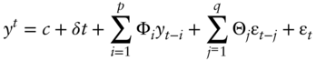
- Vector autoregression moving average with exogenous inputs VARMAX(p, q)

- Structural vector autoregression moving average SVARMA(p, q)

The following variables appear in the equations:
- yt is the vector of response time series variables at time t. yt has n elements.
- c is a constant vector of offsets, with n elements.
- Φi are n‐by‐n matrices for each i, where Φi are autoregressive matrices. There are p autoregressive matrices and some can be entirely composed of zeros.
- ɛt is a vector of serially uncorrelated innovations, vectors of length n. The t are multivariate normal random vectors with a covariance matrix Σ.
- Θj are n‐by‐n matrices for each j, where Θj are moving average matrices. There are q moving average matrices and some can be entirely composed of zeros.
- δ is a constant vector of linear time trend coefficients, with n elements.
- xt is an r‐by‐1 vector representing exogenous terms at each time t and r is the number of exogenous series. Exogenous terms are data (or other unmodelled inputs) in addition to the response time series yt. Each exogenous series appears in all response equations.
- β is an n‐by‐r constant matrix of regression coefficients of size r. So the product βxt is a vector of size n.
LSTMs provide a very interesting non‐linear version of these standard models. This paper uses multivariate LSTMs with exogenous variables in a stock picking prediction context in experiment 2.
13.3.2 Machine learning models in finance
Machine learning models have gained momentum in finance applications over the past five years following the tremendous success in areas like image recognition and natural language processing. These models have proven to be very useful to model unstructured data. In addition to that, machine learning models are able to model flexibly non‐linearity in classification and regression problems and discover hidden structure in supervised learning. Combinations of weak learners like XGBoost and AdaBoost are especially popular. Unsupervised learning is a branch of machine learning used to draw inferences from datasets consisting of input data without labelled responses – principal component analysis is an example. The challenges of using machine learning in finance are important as, like other models, it needs to deal with estimation risk, potentially non‐stationarity, overfitting and in some cases interpretability issues.
13.4 DEEP LEARNING
Deep learning is a popular area of research in machine learning, partly because it has achieved big success in artificial intelligence, in the areas of computer vision, natural language processing, machine translation and speech recognition, and partly because now it is possible to build applications based on deep learning. Everyday applications based on deep learning are recommendation systems, voice assistants and search engine technology based on computer vision, to name just a few. This success has been possible thanks to the amount of data, which today is referred to as big data, now available and the possibility to perform computation much faster than ever before. Today it is possible to port computation from the computer's central processing unit (CPU) to its graphical processing unit (GPU). Another approach is to move computations to clusters of computers in local networks or in the cloud.
The term deep learning is used to describe the activity of training deep neural networks. There are many different types of architectures and different methods for training these models. The most common network is the feed‐forward neural network (FNN) used for data that is assumed to be independent and identical distributed (i.i.d.). RNNs, meanwhile, are more suitable for sequential data, such as time series, speech data, natural language data (Bengio et al. n.d.) and other data where the assumption of i.i.d. is not fulfilled. In deep learning, the main task is to learn or approximate some function f that maps inputs x to outputs y. Deep learning tries to solve the following learning problem ŷ = f(θ;x) where x is the input to the neural network, ŷ is its output and θ is a set of parameters that gives the best fit of f. In regression, ŷ would be represented by real numbers whereas in classification it would be represented by probabilities assigned to each class in a discrete set of values.
13.4.1 Deep learning and time series
Time series models in finance need to deal with autocorrelation, volatility clustering, non‐Gaussianity, and possibly cycles and regimes. Deep learning and RNNs in particular can help model these stylized facts. On this account, an RNN is a more flexible model, since it encodes the temporal context in its feedback connections, which are capable of capturing the time varying dynamics of the underlying system (Bianchi et al. n.d.; Schäfer and Zimmermann 2007). RNNs are a special class of neural networks characterized by internal self‐connections which in principle can approximate or model any nonlinear dynamical system, up to a given degree of accuracy.
13.5 RECURRENT NEURAL NETWORKS
13.5.1 Introduction
RNNs are suitable for processing sequences, where the input might be a sequence (x1,x2,…,xT) with each datapoint xt being a real valued vector or a scalar value. The target signal (y1,y2,…,yT) can also be a sequence or a scalar value. The RNN architecture is different from that of a classical neural network. It has a recurrent connection or feedback with a time delay. The recurrent connections represent the internal states that encode the history of the sequence processed by the RNN (Yu and Deng 2015). The feedback can be implemented in many ways. Some common examples of the architecture of RNNs are taking the output from the hidden layer and feeding it back to the hidden layer together with new arriving input. Another form of recurrent feedback is taking the output signal from the network at time step t − 1 and feeding it as new input together with new input at time step t (Goodfellow et al. 2016).
An RNN has a deep architecture when unfolding it in time (Figure 13.1), where its depth is as long as the temporal input to the network. This type of depth is different from a regular deep neural network, where depth is achieved by stacking layers of hidden units on top of each other. In a sense, RNNs can be considered to have depth in both time and feature space, where depth in feature space is achieved by stacking layers of hidden units on top of each other. There even exist multidimensional RNNs suitable for video processing, medical imaging and other multidimensional sequential data (Graves 2012). RNNs have been successful for modelling variable length sequences, such as language modelling (Graves 2012; Sutskever 2013), learning word embeddings (Mokolov et al. 2013) and speech recognition (Graves 2012).

Figure 13.1 Recurrent neural network unrolled in time.
13.5.2 Elman recurrent neural network
The Elman recurrent neural network (ERNN), also known as simple RNN or vanilla RNN, is considered to be the most basic version of RNN. Most of the more complex RNN architectures, such as LSTM and gated recurrent units (GRUs), can be interpreted as a variation or as an extension of ERNNs. ERNNs have been applied in many different contexts. In natural language processing applications, ERNNs demonstrated to be capable of learning grammar using a training set of unannotated sentences to predict successive words in the sentence (Elman 1995; Ogata et al. 2007). Mori and Ogasawara (1993) studied ERNN performance in short‐term load forecasting and proposed a learning method, called ‘diffusion learning’ (a sort of momentum‐based gradient descent), to avoid local minima during the optimization procedure. Cai et al. (2007) trained an ERNN with a hybrid algorithm that combines particle swarm optimization and evolutionary computation to overcome the local minima issues of gradient‐based methods.
The layers in an RNN can be divided in an input layer, one or more hidden layers and an output layer. While input and output layers are characterized by feed‐forward connections, the hidden layers contain recurrent ones. At each time step t, the input layer process the component ![]() of a serial input x. The time series x has length T and it can contain real values, discrete values, one‐hot vectors and so on. In the input layer, each component x[t] is summed with a bias vector
of a serial input x. The time series x has length T and it can contain real values, discrete values, one‐hot vectors and so on. In the input layer, each component x[t] is summed with a bias vector ![]() , where Nh is the number of nodes in the hidden layer, and then is multiplied with the input weight matrix
, where Nh is the number of nodes in the hidden layer, and then is multiplied with the input weight matrix ![]() .
.
The internal state of the network ![]() from the previous time interval is first summed with a bias vector
from the previous time interval is first summed with a bias vector ![]() and then multiplied by the weight matrix
and then multiplied by the weight matrix ![]() of the recurrent connections. The transformed current input and past network state are then combined and processed by the neurons in the hidden layers, which apply a non‐linear transformation. The difference equations for the update of the internal state and the output of the network at a time step t are:
of the recurrent connections. The transformed current input and past network state are then combined and processed by the neurons in the hidden layers, which apply a non‐linear transformation. The difference equations for the update of the internal state and the output of the network at a time step t are:
where f(·) is the activation function of the neurons, usually implemented by a sigmoid or by a hyperbolic tangent. The hidden state h[t], which conveys the content of the memory of the network at time step t, is typically initialized with a vector of zeros and it depends on past network states and inputs. The output ![]() is computed through a transformation g(·), usually linear in a regression setting or non‐linear for classification problems using the matrix of the output weights
is computed through a transformation g(·), usually linear in a regression setting or non‐linear for classification problems using the matrix of the output weights ![]() applied to the current state h[t] and the bias vector
applied to the current state h[t] and the bias vector ![]() . All the weight matrices and biases can be trained through gradient descent, with the back‐propagation through time (BPPT) procedure. Unless differently specified, in the following to compact the notation we omit the bias terms by assuming x = [x;1], h = [h;1], y = [y;1] and by augmenting
. All the weight matrices and biases can be trained through gradient descent, with the back‐propagation through time (BPPT) procedure. Unless differently specified, in the following to compact the notation we omit the bias terms by assuming x = [x;1], h = [h;1], y = [y;1] and by augmenting ![]() , Who with an additional column.
, Who with an additional column.
13.5.3 Activation function
Activation functions are used in neural networks to transform the input of a neural network, expressed as a linear combination of weights and bias, to an output in feature space
where T denotes the transpose of the weight matrix. In the forward pass these transformations are propagated forward and eventually reach the last layer of the network and become the output of the whole network. This transformation is what makes neural networks learn nonlinear functions. The rectified linear unit (ReLu) (Figure 13.2) is the most common type of hidden unit used in modern neural networks (Goodfellow et al. 2016). It is defined as g(z) = max{0,z}.

Figure 13.2 The rectified linear unit (ReLu) and sigmoid functions.
Another activation function is the logistic sigmoid, σ(x) = (1 + exp.(−x))−1, which is a differentiable squashing function (see Figure 13.2). One of its drawbacks is that learning becomes slow due to saturations when its argument either becomes too negative or when it becomes too big. Nowadays its use is discouraged, especially in feed‐forward neural networks (Goodfellow et al. 2016). In RNNs the logistic sigmoid can be used as hidden as well as output units. The tanh(x) is very similar to the sigmoid but with a range in the interval (−1,1). It is employed as an activation function in all types of neural networks: FNN, RNN, LSTM.
13.5.4 Training recurrent neural networks
We start this section with a short introduction to the training procedure of an RNN. In order to train an RNN, we need to compute the cost function in the forward pass. Then we back‐propagate the errors committed by the network and use those errors to optimize the parameters of the model, with gradient descent.
The algorithm used to compute the gradients, in the context of RNNs, is called Backpropagation Through Time (BPTT). We introduce the loss and cost functions, then we show how the parameters of the model are updated and finally we present the BPTT algorithm.
13.5.5 Loss function
The loss function measures the discrepancy between the predictions made by the neural network and the target signal in the training data. To assess whether our model is learning we compute the cost (see below) during training and test its generalization power on a test set not seen by the model during training. Depending on the prediction task on which we want to apply our RNN, there are several loss functions to choose from. In what follows we make use of the following definitions. Let y be the target signal and f(x,θ) the output from the network. Then for a binary classification task the target belongs to the set y = {0,1}. In this case the loss function is given by (Bishop 2006):

Its derivation is as follows. An outcome from a binary classification problem is described by a Bernoulli distribution p(y ∣ x, θ) = f(x, θ)y(1 − f(x, θ))1 − y. Taking the natural logarithm on the Bernoulli distribution gives a likelihood function, which in this case is equal to the cost function, giving the stated result. In this case the output is given by f = σ(a) = (1 + exp(−a))−1 satisfying 0 ≤ f(x,θ) ≤ 1. For multi‐class classification we often use the loss function

where the output of our model is given by the softmax function

subject to the conditions 0 ≤ fk ≤ 1 and Pk fk = 1. In regression estimation tasks we make use of the mean‐squared error as the loss function (Bishop 2006)

where fn is the output of the network, xn are input vectors, with n = 1,…,N, and yn are the corresponding target vectors. In unsupervised learning, one of the main tasks is that of finding the density p(x,θ) from a set of densities such that we minimize the loss function (Vapnik 2000)
13.5.6 Cost function
Learning is achieved by minimizing the empirical risk. The principle of risk minimization can be defined as follows (Vapnik 2000). Define the loss function L(y,(x,θ)) as the discrepancy between the learning machine's output and the target signal y. The risk functional or cost function is then defined as

where F(x,y) is a joint probability distribution. The machine learning algorithm then has to find the best function f that minimizes the cost function. In practice, we have to rely on minimizing the empirical risk due to the fact that the joint distribution is unknown for the data generating process (Goodfellow et al. 2016). The empirical cost function is given by
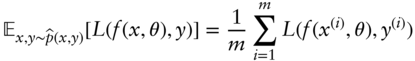
where the expectation, E, is taken over the empirical data distribution ∧p(x,y).
13.5.7 Gradient descent
To train RNNs we make use of gradient descent, an algorithm for finding the optimal point of the cost function or objective function, as it is also called. The objective function is a measure of how well the model compares to the real target. For computing gradient descent we need to compute the derivatives of the cost function with respect to the parameters. This can be achieved, for training RNNs, by employing BPTT, shown later in this section. As stated before, we are going to ignore the derivations for the bias terms. Similar identities can be obtained from the ones for the weights.
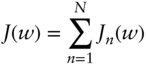
The name gradient descent refers to the fact that the updating rule for the weights chooses to take its next step in the direction of steepest gradient in weight space. To understand what this means, let us think of the loss function J(w) as a surface spanned by the weights w. When we take a small step w + δw away from w, the loss function changes as δJ 'δwT ΔJ(w). Then the vector ΔJ(w) points in the direction of greatest rate of change (Bishop 2006). Optimization amounts to finding the optimal point where the following condition holds:
If at iteration n we don't find the optimal point, we can continue downhill the surface spanned by w in the direction −ΔJ(w), reducing the loss function until we eventually find the optimal point. In the context of deep learning, it is very difficult to find a unique global optimal point. The reason is that the deep neural networks used in deep learning are compositions of functions of the input, the weights and the biases. This function composition spanning many layers of hidden units makes the cost function to be a nonlinear function of the weights and biases, thus leaving us with a non‐convex optimization problem. Gradient descent is given by
where η is the learning rate. In this form, gradient descent processes all the data at once to do an update of the weights. This form of learning is called batch learning and refers to the fact that the whole training set is used at each iteration for updating the parameters (Bishop 2006; Haykin 2009). Batch learning is discouraged (Bishop 2006, p. 240) for gradient descent as there are better batch optimization methods, such as conjugate gradients or quasi‐Newton methods (Bishop 2006). It is more appropriate to use gradient descent in its online learning version (Bishop 2006; Haykin 2009). This means simply that the parameters are updated using some portion of the data or a single point at a time after each iteration. The cost function takes the form
where the sum runs over each data point. This leads to the online or stochastic gradient descent algorithm
Its name, stochastic gradient descent, derives from the fact that the update of parameters happens either one training example at a time or by choosing points at random with replacement (Bishop 2006).
13.5.7.1 Back‐Propagation Through Time The algorithm to compute the gradients used in gradient descent, in the case of the RNN, is called BPTT. It is similar to the regular back‐propagation algorithm used to train regular FNNs. By unfolding the RNN in time we can compute the gradients by propagating the errors backward in time. Let us define the cost function as the sum of squared errors (Yu and Deng 2015):

where τt represents the target signal and yt the output from the RNN. The sum over the t variable runs over time steps t = 1,t,…,T and the sum over j runs over the j units. To further simplify notation let us redefine the equations of the RNN as:
Employing the local potentials or activation potentials ut = W T ht−1 + UT xt and vt = V T ht, by way of Eqs. (13.3) and (13.4) and using θ = {W,U,V}, we can define the errors (Yu and Deng 2015)


as the gradient of the cost function with respect to the units' potentials. The BPTT proceeds iteratively to compute the gradients over the time steps, t = T down to t = 1. For the final time step we compute

for the set of units j = 1,2,…,L. This error term can be expressed in vector notation as follows:
where is the element‐wise Hadamard product between matrices. For the hidden layers we have:

for j = 1,2,…,N. This expression can also be written in vector form as
Iterating for all other time steps t = T − 1,T − 2,…,1 we can summarize the error for the output as:
for all units j = 1,2,…,L. Similarly, for the hidden units we can summarize the result as
where ![]() is propagated from the output layer at time t and
is propagated from the output layer at time t and ![]() is propagated back from the hidden layer at time step t + 1.
is propagated back from the hidden layer at time step t + 1.
13.5.7.2 Regularization Theory Regularization theory for ill‐posed problems tries to address the question of whether we can prevent our machine learning model from overfitting and therefore plays a big role in deep learning.
In the early 1900s it was discovered that solutions to linear operator equations of the form (Vapnik 2000)
for a linear operator A and a set of functions f ∈ Γ, in an arbitrary function space Γ were ill‐posed. That the above equation is ill‐posed means that a small deviation like changing F by Fδ satisfying kF − Fδk < δ for δ arbitrary small leads kfδ − fk to become large. In the expression for the functional R(f) = kAf − Fδk2, if the functions fδ minimize the functional R(f), there is no guarantee that we find a good approximation to the right solution even if δ → 0.
Many problems in real life are ill‐posed, e.g. when trying to reverse the cause‐effect relations, a good example being to find unknown causes from known consequences. This problem is ill‐posed even though it is a one‐to‐one mapping (Vapnik 2000). Another example is that of estimating the density function from data (Vapnik 2000). In the 1960s it was recognized that if one instead minimizes the regularized functional (Vapnik 2000)
where Ω(f) is a functional and γ(δ) is a constant, then we obtain a sequence of solutions that converges to the correct solution as δ → 0. In deep learning, the first term in the functional, R*(f), will be replaced by the cost function, whereas the regularization term depends on the set of parameters θ to be optimized. For L1 regularization γ(δ)Ω(f) = λ![]() whereas for L2 regularization, this term equals
whereas for L2 regularization, this term equals ![]() (see Bishop 2006; Friedman et al. n.d.).
(see Bishop 2006; Friedman et al. n.d.).
13.5.7.3 Dropout Dropout is a type of regularization which prevents neural networks from overfitting (Srivastava et al. 2014). This type of regularization is also inexpensive (Goodfellow et al. 2016), especially when it comes to training neural networks. During training, dropout samples from an exponentially number of different thinned networks (Srivastava et al. 2014). At test time the model is an approximation of the average of all the predictions of all thinned networks only that it is a much smaller model with less weights than the networks used during training. If we have a network with L hidden layers, then l ∈ {1,…,L} is the index of each layer. If z(l) is the input to layer l, then y(l) is the output from that layer, with y(0) = x denoting the input to the network. Let W(l) denote the weights and b(l) denote the bias, then the network equations are given by:
where f is an activation function. Dropout is then a factor that randomly gets rid of some of the outputs from each layer by doing the following operation (Srivastava et al. 2014):

where * denotes element‐wise multiplication.
13.6 LONG SHORT‐TERM MEMORY NETWORKS
The LSTM architecture was originally proposed by Hochreiter and Schmidhuber (1997) and is widely used nowadays due to its superior performance in accurately modelling both short‐ and long‐term dependencies in data. For these reasons we choose the LSTM architecture over the vanilla RNN network.
When computing the gradients with BPTT, the error flows backwards in time. Because the same weights are used at each time step in an RNN, its gradients depend on the same set of weights, which causes the gradients to either grow without bound or vanish (Goodfellow et al. 2016; Hochreiter and Schmidhuber 1997; Pascanu et al. 2013). In the first case the weights oscillate; in the second, learning long time lags takes a prohibitive amount of time (Hochreiter and Schmidhuber 1997). In the case of exploding gradients there is a solution referred to as clipping the gradients (Pascanu et al. 2013), given by the procedure below, where ∧g is the gradient, δ is a threshold and L is the loss function. But the vanishing gradient problem did not seem to have a solution. To solve this problem, Hochreiter and Schmidhuber (1997) introduced the LSTM network, similar to the RNN but where the hidden units are replaced by memory cells. The LSTM is an elegant solution to the vanishing and exploding gradients encountered in RNNs. The hidden cell in the LSTM (Figure 13.3) is a structure that holds an internal state with a recurrent connection of constant weight which allows the gradients to pass many times without exploding or vanishing (Lipton et al. n.d.).

Figure 13.3 Memory cell or hidden unit in an LSTM recurrent neural network.
The LSTM network is a set of subnets with recurrent connections, known as memory blocks. Each block contains one or more self‐connected memory cells and three multiplicative units known as the input, output and forget gates, which respectively support read, write and reset operations for the cells (Graves 2012). The gating units control the gradient flow through the memory cell and when closing them allows the gradient to pass without alteration for an indefinite amount of time, making the LSTM suitable for learning long time dependencies, thus overcoming the vanishing gradient problem that RNNs suffer from. We describe in more detail the inner workings of an LSTM cell. The memory cell is composed of an input node, an input gate, an internal state, a forget gate and an output gate. The components in a memory cell are as follows:
- The input node takes the activation from both the input layer, xt, and the hidden state ht−1 at time t − 1. The input is then fed to an activation function, either a tanh or a sigmoid.
- The input gate uses a sigmoidal unit that get its input from the current data xt and the hidden units at time step t − 1. The input gate multiplies the value of the input node and because it is a sigmoid unit with range between zero and one, it can control the flow of the signal it multiplies.
- The internal state has a self‐recurrent connection with unit weight, also called the constant error carousel in Hochreiter and Schmidhuber (1997), and is given by s t = gt ⊙ it + ft ⊙ st − 1. The Hadamard product denotes element‐wise product and ft is the forget gate (see below).
- The forget gate, ft, was not part of the original model for the LSTM but was introduced by Gers et al. (2000). The forget gate multiplies the internal state at time step t − 1 and in that way can get rid of all the contents in the past, as demonstrated by the equation in the list item above.
- The resulting output from a memory cell is produced by multiplying the value of the internal state sc by the output gate oc. Often the internal state is run through a tanh activation function.
The equations for the LSTM network can be summarized as follows. As before, let g stand for the input to the memory cell, i for the input gate, f for the forget gate, o for the output gate and (Figure 13.4)

Figure 13.4 LSTM recurrent neural network unrolled in time. s for the cell state (Lipton et al. n.d.).
where the Hadamard product denotes element‐wise multiplication. In the equations, ht is the value of the hidden layer at time t, while ht−1 is the output by each memory cell in the hidden layer at time t − 1. The weights {WgX,WiX,WfX,WoX} are the connections between the inputs xt with the input node, the input gate, the forget gate and the output gate respectively. In the same manner, {Wgh,Wih,Wfh,Woh} represent the connections between the hidden layer with the input node, the input gate, the forget gate and the output gate respectively. The bias terms for each of the cell's components is given by {bg,bi,bf,bo}.
13.7 FINANCIAL MODEL
The goal with this work is to predict the stock returns for 50 stocks from the S&P 500. As input to the model we used the stock returns up to time t and the prediction from the model, an LSTM, is the stock returns at time t + 1. The predictions from the model help us decide at time t which stocks to buy, hold or sell. This way we have an automated trading policy. For stock i we predict the return at time t + 1 using historical returns up to time t.
13.7.1 Return series construction
The returns are computed as:

where Pti is the price at time t for stock or commodity i and Rti+1 is its return at time t + 1. Our deep learning model then tries to learn a function Gθ(·) for predicting the return at time t + 1 for a parameter set θ:
where k is the number of time steps backward in time for the historical returns. We used a rolling window of 30 daily returns to predict the return for day 31 on a rolling basis. This process generated sequences of 30 consecutive one‐day returns ![]() , where t ≥ 30 for all of stocks i.
, where t ≥ 30 for all of stocks i.
13.7.2 Evaluation of the model
One solution to machine learning‐driven investing with the use of deep learning would be to build a classifier with class 0 denoting negative returns and class 1 denoting positive returns. However, in our experiments we observed that solving the problem with regression gave better results than using pure classification. When learning our models, we used the mean squared error (MSE) loss as objective function. First, after the models were trained and validated with a validation set, we made predictions on an independent test set, or as we call it here, live dataset. These predictions were tested with respect to the target series of our stock returns (see experiments 1 and 2) on the independent set, with a measure for correctness called the hit ratio. In line with Lee and Yoo (2017), we chose the HR as a measure of how correct the model predicts the outcome of the stock returns compared to the real outcome. The HR is defined as:

where N is the total number of trading days and Ut is defined as:

where Rt in the realized stock returns and ![]() is the predicted stock returns at trading day t. Thus, HR is the rate of correct predictions measured against the real target series. By using the HR as a measure of discrepancy we could conclude that the predictions either moved in the same direction as the live target returns or moved in the opposite direction. If HR equals one, it indicates perfect correlation and a value of zero indicates that the prediction and the real series moved in opposite directions. A value of HR > 0.50 indicates that the model is right more than 50% of the time while a value of HR ≤ 0.50 indicates that the model guesses the outcome.
is the predicted stock returns at trading day t. Thus, HR is the rate of correct predictions measured against the real target series. By using the HR as a measure of discrepancy we could conclude that the predictions either moved in the same direction as the live target returns or moved in the opposite direction. If HR equals one, it indicates perfect correlation and a value of zero indicates that the prediction and the real series moved in opposite directions. A value of HR > 0.50 indicates that the model is right more than 50% of the time while a value of HR ≤ 0.50 indicates that the model guesses the outcome.
For the computations we used Python, as well as Keras and PyTorch deep learning libraries. Keras and PyTorch use tensors with strong GPU acceleration. The GPU computations were performed both on an NVIDIA GeForce GTX 1080 Ti and an NVIDIA GeForce GTX 1070 GDDR5 card on two separate machines.
13.7.3 Data and results
We conducted two types of experiments. The first was intended to demonstrate the predictive power of the LSTM using one stock at a time as input up to time t and as target the same stock's returns at time t + 1. From now on we refer to it as experiment 1. The second experiment was intended to predict the returns for all stocks simultaneously. This means that all of our 50 stock returns up to time t were fed as input to an LSTM which was trained to predict the 50 stock returns at time t + 1. Additionally, to the 50 stocks we fed to the model the returns from crude oil futures, silver and gold returns. We refer to this as experiment 2. All the stocks used in this chapter are from the S&P 500, while the commodity prices were from data provider Quandl (Quandl n.d.).
13.7.3.1 Experiment 1
13.7.3.1.1 Main Experiments For experiment 1, our model used the stock returns as input up to time t, one at a time, to predict the same returns at time t + 1 – see the discussion above on return series construction. A new model was trained for each stock. Most of the parameters where kept constant during training for every stock. The learning rate was set to 0.001 and we used a dropout rate of 0.01, the only exception being the number of hidden units. The number of hidden units is different for different stocks. For every stock we started with an LSTM with 100 hidden units and increased that number until the condition HR > 0.70 was met, increasing the number of units with 50 units per iteration up to 200 hidden units.
Note that the condition HR > 0.70 was never met, but this value was chosen merely to keep the computations running until an optimum was found. At most we ran the experiments for 400 epochs but stopped if there was no improvement in the test error or if the test error increased. This technique is called early stopping. For early stopping we used a maximum number of 50 epochs before stopping the training. The training was performed in batches of 512.
Because we trained different LSTMs for different stocks, we ended up with different amounts of data for training, testing and validating the models. Sometimes we refer to the test data as live data. The data was divided first in 90% to 10%, where the 10% portion was for testing (live data) and corresponded to the most recent stock prices. The 90% portion was then divided once again in 85% to 15% for training and validation respectively. The number of data points and periods for the datasets are given in the appendix in Table 13.A.1. For optimization we tested both the RMSProp and Adam algorithms, but found that the best results were achieved with stochastic gradient descent and momentum. This is true only when processing one time series at a time. For experiment 2 we used the Adam optimization algorithm. The results from experiment 1 are shown in Table 13.1.
Table 13.1 Experiment 1: comparison of performance measured as the HR for LSTM, SVM and NN
| Stock | Hidden units | HR LSTM | HR SVM | HR NN |
| AAPL | 150 | 0.53 | 0.52 | 0.52 (130) |
| MSFT | 100 | 0.51 | 0.49 | 0.49 (150) |
| FB | 100 | 0.58 | 0.58 | 0.56 (90) |
| AMZN | 100 | 0.55 | 0.56 | 0.53 (90) |
| JNJ | 100 | 0.52 | 0.47 | 0.50 (50) |
| BRK/B | 150 | 0.51 | 0.51 | 0.51 (50) |
| JPM | 100 | 0.52 | 0.51 | 0.50 (90) |
| XOM | 100 | 0.52 | 0.52 | 0.49 (50) |
| GOOGL | 100 | 0.54 | 0.53 | 0.53 (70) |
| GOOG | 100 | 0.55 | 0.55 | 0.55 (50) |
| BAC | 100 | 0.47 | 0.50 | 0.59 (50) |
| PG | 100 | 0.50 | 0.50 | 0.50 (110) |
| T | 150 | 0.52 | 0.48 | 0.50 (70) |
| WFC | 150 | 0.51 | 0.47 | 0.50 (70) |
| GE | 100 | 0.51 | 0.50 | 0.50 (110) |
| CVX | 150 | 0.50 | 0.53 | 0.50 (70) |
| PFE | 100 | 0.49 | 0.49 | 0.49 (50) |
| VZ | 150 | 0.51 | 0.53 | 0.50 (50) |
| CMCSA | 150 | 0.54 | 0.49 | 0.50 (110) |
| UNH | 100 | 0.52 | 0.48 | 0.52 (130) |
| V | 100 | 0.59 | 0.51 | 0.55 (70) |
| C | 150 | 0.52 | 0.50 | 0.51 (50) |
| PM | 100 | 0.56 | 0.56 | 0.52 (110) |
| HD | 100 | 0.53 | 0.50 | 0.53 (70) |
| KO | 150 | 0.51 | 0.48 | 0.50 (70) |
| MRK | 200 | 0.54 | 0.49 | 0.50 (110) |
| PEP | 100 | 0.55 | 0.52 | 0.51 (50) |
| INTC | 150 | 0.53 | 0.45 | 0.51 (110) |
| CSCO | 100 | 0.51 | 0.48 | 0.50 (90) |
| ORCL | 150 | 0.52 | 0.48 | 0.50 (130) |
| DWDP | 150 | 0.51 | 0.48 | 0.50 (90) |
| DIS | 150 | 0.53 | 0.49 | 0.52 (130) |
| BA | 100 | 0.54 | 0.53 | 0.51 (50) |
| AMGN | 100 | 0.51 | 0.52 | 0.53 (90) |
| MCD | 150 | 0.55 | 0.48 | 0.52 (130) |
| MA | 100 | 0.57 | 0.57 | 0.55 (130) |
| IBM | 100 | 0.49 | 0.49 | 0.50 (50) |
| MO | 150 | 0.55 | 0.47 | 0.52 (50) |
| MMM | 100 | 0.53 | 0.46 | 0.52 (90) |
| ABBV | 100 | 0.60 | 0.38 | 0.41 (110) |
| WMT | 100 | 0.52 | 0.50 | 0.51 (50) |
| MDT | 150 | 0.52 | 0.49 | 0.50 (50) |
| GILD | 100 | 0.50 | 0.52 | 0.51 (70) |
| CELG | 100 | 0.51 | 0.52 | 0.50 (90) |
| HON | 150 | 0.55 | 0.46 | 0.52 (130) |
| NVDA | 100 | 0.56 | 0.55 | 0.54 (90) |
| AVGO | 100 | 0.57 | 0.57 | 0.51 (130) |
| BMY | 200 | 0.52 | 0.49 | 0.50 (50) |
| PCLN | 200 | 0.54 | 0.54 | 0.53 (70) |
| ABT | 150 | 0.50 | 0.47 | 0.50 (70) |
The results are computed for the independent live dataset. The numbers in parentheses in the NN column stand for the number of hidden units.
13.7.3.1.2 Baseline Experiments The LSTM model was compared to two other models. The baseline models were a support vector machine (SVM) (Friedman et al. n.d.) and a neural network (NN). The NN consisted of one hidden layer, where the number of hidden units were chosen with the same procedure as that for the LSTM, the only difference being that the range for choosing hidden units lies in the range 50–150. Additionally, we used the same learning rate, number of epochs, batch size and drop rate as those used for the LSTM. For the NNs we trained the models in a regression setting using the MSE. For the predictions produced by the NN we computed the HR on the live dataset. The results are presented together with those for the LSTM in Table 13.1.
By inspecting Table 13.1 we can get the following figures. The LSTM achieved a value HR > 0.50 for 43 stocks out of 50 and did not better than chance (HR ≤ 0.50) for the remaining 7 stocks. The SVM got it ‘right’ (HR > 0.50) for 21 stocks, while the NN did just a little better with 27 stocks moving in the same direction as the true series. If we imagine that HR = 0.51 can be achieved by rounding the results, those values can be questioned as also being achieved by chance. The LSTM had a value of HR = 0.51 for 10 stocks, the SVM for 3 stocks while the NN for 8 stocks. Even if the LSTM seems superior to the other models, the difference in performance is not that big, except for some cases. On some stocks both the SVM and the NN can be as good as the LSTM or better. But what this experiment shows is that the LSTM is consistent in predicting the direction in which its predictions move with respect to the real series.
13.7.3.2 Experiment 2
In this experiment we used the returns of all the 50 stocks. Additionally, we used oil, gold and S&P 500 return series of the 30 previous days as input. The output from our model is the prediction of the 50 stock returns. To test the robustness of the LSTM we also performed experiments against a baseline model, which in this case consisted of an SVM (Friedman et al. n.d.), suited for regression. To test the profitability of the LSTM, we ran experiments on a smaller portfolio consisting of 40 of our initial stocks (see Table 13.4) and the return series from the S&P 500, oil and gold. This part of the experiment is intended to show that the LSTM is consistent in its predictions independent of the time periods. Especially we were interested to see whether the model was robust to the subprime financial crisis. These results are shown in Table 13.5.
Because this section consists of many experiments, we present the experiment performed on the 50 stocks plus commodities in the main experiment subsection. The baseline experiment is presented in the subsection above and the last experiment for time periods in the ‘Results in different market regimes’ subsection below.
13.7.3.2.1 Main Experiment All the features in this experiment were scaled with the min‐max formula:
where  , and a, b is the range (a,b) of the features. It is common to set a = 0 and b = 1. The training data consisted of 560 days from the period 2014‐05‐13 to 2016‐08‐01. We used a validation set consisting of 83 days for choosing the meta parameters, from the period 2016‐08‐02 to 2016‐11‐25 and a test set of 83 days from the period 2016‐11‐28 to 2017‐03‐28. Finally, we used a live dataset of 111 days for the period 2017‐03‐29 to 2017‐09‐05.
We used an LSTM with one hidden layer LSTM and 50 hidden units. As activation function we used the ReLu; we also used a dropout rate of 0.01 and a batch size of 32. The model was trained for 400 epochs. The parameters of the Adam optimizer were a learning rate of 0.001, β1 = 0.9, β2 = 0.999, ɛ = 10−9 and the decay parameter was set to 0.0 As loss function we used the MSE.
To assess the quality of our model and to try to determine whether it has value for investment purposes, we looked at the ‘live dataset’, which is the most recent dataset. This dataset is not used during training and can be considered to be an independent dataset. We computed the HR on the predictions made with the live data to assess how often our model was right compared to the true target returns. The hit ratio gives us information if the predictions of the model move in the same direction as the true returns. To evaluate the profitability of the model we built daily updated portfolios using the predictions from the model and computed their average daily return. A typical scenario would be that we get predictions from our LSTM model just before market opening for all 50 daily stock returns. According to the direction predicted, positive or negative, we open a long position in stock i if Rti > 0. If Rti < 0 we can either decide to open a short position (in that case we call it a long‐short portfolio) for stock i or do nothing and if we own the stocks we can choose to keep them (we call it a long portfolio). At market closing we close all positions. Thus, the daily returns of the portfolio on day t for a long‐short portfolio is ![]() .
.
Regarding the absolute value of the weights for the portfolio we tried two kinds of similar, equally‐weighted portfolios. Portfolio 1: at the beginning we allocate the same proportion of capital to invest in each stock, then the returns on each stock are independently compounded, thus the portfolio return on a period is the average of the returns on each stock on the period. Portfolio 2: the portfolio is rebalanced each day, i.e. each day we allocate the same proportion of capital to invest in each stock, thus the portfolio daily return is the average of the daily returns on each stock. Each of the portfolios has a long and a long‐short version. We are aware that not optimizing the weights might result in very conservative return profiles in our strategy. The results from experiment 2 are presented in Table 13.2.
Table 13.2 Experiment 2 (main experiment)
| Stock | HR | Avg Ret %(L) | Avg Ret %(L/S) |
| Portfolio 1 | 0.63 | 0.18 | 0.27 |
| Portfolio 2 | 0.63 | 0.18 | 0.27 |
| AAPL | 0.63 | 0.24 | 0.32 |
| MSFT | 0.71 | 0.29 | 0.45 |
| FB | 0.71 | 0.31 | 0.42 |
| AMZN | 0.69 | 0.27 | 0.41 |
| JNJ | 0.65 | 0.12 | 0.19 |
| BRK/B | 0.70 | 0.19 | 0.31 |
| JPM | 0.62 | 0.22 | 0.38 |
| XOM | 0.70 | 0.11 | 0.25 |
| GOOGL | 0.72 | 0.31 | 0.50 |
| GOOG | 0.75 | 0.32 | 0.52 |
| BAC | 0.70 | 0.30 | 0.55 |
| PG | 0.60 | 0.60 | 0.90 |
| T | 0.61 | 0.80 | 0.22 |
| WFC | 0.67 | 0.16 | 0.38 |
| GE | 0.64 | 0.50 | 0.24 |
| CVX | 0.71 | 0.18 | 0.31 |
| PFE | 0.66 | 0.70 | 0.14 |
| VZ | 0.50 | 0.10 | 0.10 |
| CMCSA | 0.63 | 0.23 | 0.36 |
| UNH | 0.59 | 0.20 | 0.22 |
| V | 0.65 | 0.23 | 0.31 |
| C | 0.69 | 0.28 | 0.39 |
| PM | 0.64 | 0.17 | 0.28 |
| HD | 0.61 | 0.10 | 0.17 |
| KO | 0.61 | 0.80 | 0.90 |
| MRK | 0.61 | 0.90 | 0.16 |
| PEP | 0.60 | 0.80 | 0.11 |
| INTC | 0.63 | 0.16 | 0.31 |
| CSCO | 0.68 | 0.14 | 0.31 |
| ORCL | 0.52 | 0.80 | 0.40 |
| DWDP | 0.60 | 0.21 | 0.35 |
| DIS | 0.59 | 0 | 0.90 |
| BA | 0.57 | 0.23 | 0.16 |
| AMGN | 0.65 | 0.21 | 0.36 |
| MCD | 0.58 | 0.16 | 0.12 |
| MA | 0.66 | 0.25 | 0.34 |
| IBM | 0.54 | −0.40 | 0.60 |
| MO | 0.59 | 0.10 | 0.13 |
| MMM | 0.63 | 0.16 | 0.24 |
| ABBV | 0.61 | 0.18 | 0.22 |
| WMT | 0.50 | 0.14 | 0.16 |
| MDT | 0.59 | 0.90 | 0.17 |
| GILD | 0.50 | 0.16 | 0.11 |
| CELG | 0.64 | 0.28 | 0.45 |
| HON | 0.66 | 0.15 | 0.20 |
| NVDA | 0.68 | 0.54 | 0.68 |
| AVGO | 0.65 | 0.37 | 0.59 |
| BMY | 0.57 | 0.13 | 0.19 |
| PCLN | 0.61 | 0.14 | 0.24 |
| ABT | 0.63 | 0.21 | 0.28 |
HR, average daily returns for long portfolio (L) and long‐short portfolio (L/S) in percent. The results are computed for the independent live dataset.
13.7.3.2.2 Baseline Experiments This experiment was designed first to compare the LSTM to a baseline, in this case an SVM, and second to test the generalization power between the models with respect to the look‐back period used as input to the LSTM and the SVM. We noticed that using a longer historic return series as input, the LSTM remains robust and we don't see overfitting, as is the case for the SVM. The SVM had very good performance on the training set but performed worse on the validation and test sets. Both the LSTM and the SVM were tested with a rolling window of days in the set: {1,2,5,10}.
The results of the baseline experiment are shown in Table 13.3. We can see from the results that the LSTM improves its performance in the HR and the average daily returns in both the long and long‐short portfolios. For the SVM, the opposite is true, i.e. the SVM is comparable to the LSTM only when taking into account the most recent history. The more historic data we use, the more the SVM deteriorates in all measures, HR, and average daily returns for the long and long‐short portfolios. This is an indication that the SVM overfits to the training data the longer backward in time our look‐back window goes, whereas the LSTM remains robust.
Table 13.3 Experiment 2 (baseline experiment)
| Model | HR | Avg Ret %(L) | Avg Ret %(L/S) |
| LSTM (1) | 0.59 | 0.14 | 0.21 |
| LSTM (2) | 0.61 | 0.17 | 0.26 |
| LSTM (5) | 0.62 | 0.17 | 0.26 |
| LSTM (10) | 0.62 | 0.17 | 0.26 |
| SVM (1) | 0.59 | 0.14 | 0.21 |
| SVM (2) | 0.58 | 0.13 | 0.18 |
| SVM (5) | 0.57 | 0.12 | 0.16 |
| SVM (10) | 0.55 | 0.11 | 0.14 |
The table shows the HR and the daily average returns for each model; all computations are performed on the out‐of‐sample live dataset. The number in parentheses in the model name indicates the look‐back length of the return series, i.e. trading days.
13.7.3.2.3 Results in Different Market Regimes To validate our results for this experiment, we performed another experiment on portfolio 1. This time, instead of using all 50 stocks as input and output for the model, we picked 40 stocks. As before, we added the return series for the S&P 500, oil and gold in this portfolio. The data was divided as training set 66%, validation (1) 11%, validation (2) 11%, live dataset 11%. The stocks used for this portfolio are presented in Table 13.4 and the results are shown in Table 13.5. Notice that the performance of the portfolio (Sharpe ratio) reaches a peak in the pre‐financial crisis era (2005–2008) just to decline during the crisis but still with a performance quite high. These experiments are performed with no transaction costs and we still assume that we can buy and sell without any market frictions, which in reality might not be possible during a financial crisis.
Table 13.4 Experiment 2 (stocks used for this portfolio)
| AAPL | MSFT US | AMZN US Equity | JNJ US |
| BRK/B | JPM | XOM | BAC |
| PG | T | WFC | GE |
| CVX | PFE | VZ | CMCSA |
| UNH | C | HD | KO |
| MRK | PEP | INTC | CSCO |
| ORCL | DWDP | DIS | BA |
| AMGN | MCD | IBM | MO |
| MMM | WMT | MDT | GILD |
| CELG | HON | BMY | ABT |
The 40 stocks used for the second part of experiment 2.
Table 13.5 Experiment 2 (results in different market regimes)
| Training period | HR % | Avg. Ret % (L) | Avg. Ret % (L/S) | Sharpe ratio (L) | Sharpe ratio (L/S) |
| 2000–2003 | 49.7 | −0.05 | −0.12 | −0.84 | −1.60 |
| 2001–2004 | 48.1 | 0.05 | −0.02 | 2.06 | −0.73 |
| 2002–2005 | 52.5 | 0.11 | 0.10 | 6.05 | 3.21 |
| 2003–2006 | 55.9 | 0.10 | 0.16 | 5.01 | 5.85 |
| 2004–2007 | 54.0 | 0.14 | 0.12 | 9.07 | 5.11 |
| 2005–2008 | 61.7 | 0.26 | 0.45 | 7.00 | 9.14 |
| 2006–2009 | 59.7 | 0.44 | 1.06 | 3.10 | 6.22 |
| 2007–2010 | 53.8 | 0.12 | 0.12 | 5.25 | 2.70 |
| 2008–2011 | 56.5 | 0.20 | 0.26 | 6.12 | 6.81 |
| 2009–2012 | 62.8 | 0.40 | 0.68 | 6.31 | 9.18 |
| 2010–2013 | 55.4 | 0.09 | 0.14 | 3.57 | 3.73 |
| 2011–2014 | 58.1 | 0.16 | 0.21 | 5.59 | 6.22 |
| 2012–2015 | 56.0 | 0.15 | 0.21 | 5.61 | 5.84 |
This table shows HR, average daily return for a long (L) portfolio, average daily return for a long‐short (L/S) and their respective Sharpe ratios (L) and (L/S). The results are computed for the independent live dataset. Each three‐year period is divided into 66% training, 11% validation (1), 11% validation (2) and 11% live set.
The LSTM network was trained for periods of three years and the test on live data was performed on data following the training and validation period. What this experiment intends to show is that the LSTM network can help us pick portfolios with very high Sharpe ratio independent of the time period chosen in the backtest. This means that the good performance of the LSTM is not merely a stroke of luck in the good times that stock markets are experiencing these times.
13.8 CONCLUSIONS
Deep learning has proven be one of the most successful machine learning families of models in modelling unstructured data in several fields like computer vision and natural language processing. Deep learning solves this central problem in representation learning by introducing representations that are expressed in terms of other, simpler representations. Deep learning allows the computer to build complex concepts out of simpler concepts. A deep learning system can represent the concept of an image of a person by combining simpler concepts, such as corners and contours, which are in turn defined in terms of edges.
The idea of learning the right representation for the data provides one perspective on deep learning. You can think about it as the first layers ‘discovering’ features that allow an efficient dimensionality reduction phase and perform non‐linear modelling.
Another perspective on deep learning is that depth allows computers to learn a multi‐step computer program. Each layer of the representation can be thought of as the state of the computer's memory after executing another set of instructions in parallel. Networks with greater depth can execute more instructions in sequence. Sequential instructions offer great power because later instructions can refer back to the results of earlier instructions.
Convolutional neural networks for image processing and RNNs for natural language processing are being used more and more in finance as well as in other sciences. The price to pay for these deep models is a large number of parameters to be learned, the need to perform non‐convex optimizations and the interpretability. Researchers have found in different contexts the right models to perform tasks with great accuracy, reaching stability, avoiding overfitting and improving the interpretability of these models.
Finance is a field in which these benefits can be exploited given the huge amount of structured and unstructured data available to financial practitioners and researchers. In this chapter we explore an application on time series. Given the fact that autocorrelations, cycles and non‐linearities are present in time series, LSTM networks are a suitable candidate to model time series in finance. Elman neural networks are also a good candidate for this task, but LSTMs have proven to be better in other non‐financial applications. Time series also exhibit other challenging features such as estimation and non‐stationarity.
We have tested the LSTM in a univariate context. The LSTM network performs better than both SVMs and NNs – see experiment 1. Even though the difference in performance is not very important, the LSTM shows consistency in its predictions.
Our multivariate LSTM network experiments with exogeneous variables show good performance consistent with what happens when using VAR models compared with AR models, their ‘linear’ counterpart. In our experiments, LSTMs show better accuracy ratios, hit ratios and high Sharpe ratios in our equally‐weighted long‐only and unconstrained portfolios in different market environments.
These ratios show good behaviour in‐sample and out‐of‐sample. Sharpe ratios of our portfolio experiments are 8 for the long‐only portfolio and 10 for the long‐short version, an equally‐weighted portfolio would have provided a 2.7 Sharpe ratio using the model from 2014 to 2017. Results show consistency when using the same modelling approach in different market regimes. No trading costs have been considered.
We can conclude that LSTM networks are a promising modelling tool in financial time series, especially in the multivariate LSTM networks with exogeneous variables. These networks can enable financial engineers to model time dependencies, non‐linearity, feature discovery with a very flexible model that might be able to offset the challenging estimation and non‐stationarity in finance and the potential of overfitting. These issues can never be underestimated in finance, even more so in models with a high number of parameters, non‐linearity and difficulty to interpret like LSTM networks.
We think financial engineers should then incorporate deep learning to model not only unstructured but also structured data. We have interesting modelling times ahead of us.
Appendix A
Table 13.A.1 Periods for training set, test set and live dataset in experiment 1
| Stock | Training period | Test period | Live period |
| AAPL | 1982‐11‐15 2009‐07‐08 (6692) | 2009‐07‐09 2014‐03‐18 (1181) | 2014‐03‐19 2017‐09‐05 (875) |
| MSFT | 1986‐03‐17 2010‐04‐21 (6047) | 2010‐04‐22 2014‐07‐17 (1067) | 2014‐07‐18 2017‐09‐05 (791) |
| FB | 2012‐05‐21 2016‐06‐20 (996) | 2016‐06‐21 2017‐03‐02 (176) | 2017‐03‐03 2017‐09‐05 (130) |
| AMZN | 1997‐05‐16 2012‐12‐07 (3887) | 2012‐12‐10 2015‐08‐31 (686) | 2015‐09‐01 2017‐09‐05 (508) |
| JNJ | 1977‐01‐05 2008‐02‐20 (7824) | 2008‐02‐21 2013‐08‐14 (1381) | 2013‐08‐15 2017‐09‐05 (1023) |
| BRK/B | 1996‐05‐13 2012‐09‐11 (4082) | 2012‐09‐12 2015‐07‐24 (720) | 2015‐07‐27 2017‐09‐05 (534) |
| JPM | 1980‐07‐30 2008‐12‐19 (7135) | 2008‐12‐22 2013‐12‐20 (1259) | 2013‐12‐23 2017‐09‐05 (933) |
| XOM | 1980‐07‐30 2008‐12‐19 (7136) | 2008‐12‐22 2013‐12‐20 (1259) | 2013‐12‐23 2017‐09‐05 (933) |
| GOOGL | 2004‐08‐20 2014‐08‐25 (2490) | 2014‐08‐26 2016‐05‐23 (439) | 2016‐05‐24 2017‐09‐05 (325) |
| GOOG | 2014‐03‐31 2016‐11‐22 (639) | 2016‐11‐23 2017‐05‐08 (113) | 2017‐05‐09 2017‐09‐05 (84) |
| BAC | 1980‐07‐30 2008‐12‐19 (7134) | 2008‐12‐22 2013‐12‐20 (1259) | 2013‐12‐23 2017‐09‐05 (933) |
| PG | 1980‐07‐30 2008‐12‐19 (7136) | 2008‐12‐22 2013‐12‐20 (1259) | 2013‐12‐23 2017‐09‐05 (933) |
| T | 1983‐11‐23 2009‐10‐02 (6492) | 2009‐10‐05 2014‐04‐24 (1146) | 2014‐04‐25 2017‐09‐05 (849) |
| WFC | 1980‐07‐30 2008‐12‐19 (7135) | 2008‐12‐22 2013‐12‐20 (1259) | 2013‐12‐23 2017‐09‐05 (933) |
| GE | 1971‐07‐08 2006‐11‐06 (8873) | 2006‐11‐07 2013‐01‐29 (1566) | 2013‐01‐30 2017‐09‐05 (1160) |
| CVX | 1980‐07‐30 2008‐12‐19 (7136) | 2008‐12‐22 2013‐12‐20 (1259) | 2013‐12‐23 2017‐09‐05 (933) |
| PFE | 1980‐07‐30 2008‐12‐19 (7135) | 2008‐12‐22 2013‐12‐20 (1259) | 2013‐12‐23 2017‐09‐05 (933) |
| VZ | 1983‐11‐23 2009‐10‐02 (6492) | 2009‐10‐05 2014‐04‐24 (1146) | 2014‐04‐25 2017‐09‐05 (849) |
| CMCSA | 1983‐08‐10 2009‐09‐09 (6549) | 2009‐09‐10 2014‐04‐14 (1156) | 2014‐04‐15 2017‐09‐05 (856) |
| UNH | 1985‐09‐04 2010‐03‐08 (6150) | 2010‐03‐09 2014‐06‐27 (1085) | 2014‐06‐30 2017‐09‐05 (804) |
| V | 2008‐03‐20 2015‐06‐26 (1800) | 2015‐06‐29 2016‐09‐29 (318) | 2016‐09‐30 2017‐09‐05 (235) |
| C | 1986‐10‐31 2010‐06‐14 (5924) | 2010‐06‐15 2014‐08‐08 (1046) | 2014‐08‐11 2017‐09‐05 (775) |
| PM | 2008‐03‐19 2015‐06‐26 (1801) | 2015‐06‐29 2016‐09‐29 (318) | 2016‐09‐30 2017‐09‐05 (235) |
| HD | 1981‐09‐24 2009‐03‐31 (6913) | 2009‐04‐01 2014‐02‐04 (1220) | 2014‐02‐05 2017‐09‐05 (904) |
| KO | 1968‐01‐04 2006‐01‐13 (9542) | 2006‐01‐17 2012‐09‐20 (1684) | 2012‐09‐21 2017‐09‐05 (1247) |
| MRK | 1980‐07‐30 2008‐12‐19 (7135) | 2008‐12‐22 2013‐12‐20 (1259) | 2013‐12‐23 2017‐09‐05 (933) |
| PEP | 1980‐07‐30 2008‐12‐19 (7135) | 2008‐12‐22 2013‐12‐20 (1259) | 2013‐12‐23 2017‐09‐05 (933) |
| INTC | 1982‐11‐15 2009‐07‐08 (6692) | 2009‐07‐09 2014‐03‐18 (1181) | 2014‐03‐19 2017‐09‐05 (875) |
| CSCO | 1990‐02‐20 2011‐03‐24 (5287) | 2011‐03‐25 2014‐12‐08 (933) | 2014‐12‐09 2017‐09‐05 (691) |
| ORCL | 1986‐04‐16 2010‐04‐29 (6032) | 2010‐04‐30 2014‐07‐22 (1064) | 2014‐07‐23 2017‐09‐05 (788) |
| DWDP | 1980‐07‐30 2008‐12‐19 (7135) | 2008‐12‐22 2013‐12‐20 (1259) | 2013‐12‐23 2017‐09‐05 (933) |
| DIS | 1974‐01‐07 2007‐06‐06 (8404) | 2007‐06‐07 2013‐04‐26 (1483) | 2013‐04‐29 2017‐09‐05 (1099) |
| BA | 1980‐07‐30 2008‐12‐19 (7136) | 2008‐12‐22 2013‐12‐20 (1259) | 2013‐12‐23 2017‐09‐05 (933) |
| AMGN | 1984‐01‐04 2009‐10‐13 (6473) | 2009‐10‐14 2014‐04‐29 (1142) | 2014‐04‐30 2017‐09‐05 (846) |
| MCD | 1980‐07‐30 2008‐12‐19 (7135) | 2008‐12‐22 2013‐12‐20 (1259) | 2013‐12‐23 2017‐09‐05 (933) |
| MA | 2006‐05‐26 2015‐01‐23 (2149) | 2015‐01‐26 2016‐07‐26 (379) | 2016‐07‐27 2017‐09‐05 (281) |
| IBM | 1968‐01‐04 2006‐01‐13 (9541) | 2006‐01‐17 2012‐09‐20 (1684) | 2012‐09‐21 2017‐09‐05 (1247) |
| MO | 1980‐07‐30 2008‐12‐19 (7134) | 2008‐12‐22 2013‐12‐20 (1259) | 2013‐12‐23 2017‐09‐05 (933) |
| MMM | 1980‐07‐30 2008‐12‐19 (7135) | 2008‐12‐22 2013‐12‐20 (1259) | 2013‐12‐23 2017‐09‐05 (933) |
| ABBV | 2012‐12‐12 2016‐08‐05 (888) | 2016‐08‐08 2017‐03‐22 (157) | 2017‐03‐23 2017‐09‐05 (116) |
| WMT | 1972‐08‐29 2007‐02‐09 (8664) | 2007‐02‐12 2013‐03‐08 (1529) | 2013‐03‐11 2017‐09‐05 (1133) |
| MDT | 1980‐07‐30 2008‐12‐19 (7135) | 2008‐12‐22 2013‐12‐20 (1259) | 2013‐12‐23 2017‐09‐05 (933) |
| GILD | 1992‐01‐24 2011‐09‐07 (4912) | 2011‐09‐08 2015‐02‐19 (867) | 2015‐02‐20 2017‐09‐05 (642) |
| CELG | 1987‐09‐02 2010‐08‐27 (5755) | 2010‐08‐30 2014‐09‐11 (1016) | 2014‐09‐12 2017‐09‐05 (752) |
| HON | 1985‐09‐23 2010‐03‐11 (6139) | 2010‐03‐122014‐06‐30 (1083) | 2014‐07‐01 2017‐09‐05 (803) |
| NVDA | 1999‐01‐25 2013‐05‐03 (3562) | 2013‐05‐06 2015‐10‐29 0(466) | 2015‐10‐30 2017‐09‐05 (466) |
| AVGO | 2009‐08‐07 2015‐10‐22 (1533) | 2015‐10‐23 2016‐11‐17 (271) | 2016‐11‐18 2017‐09‐05 (200) |
| BMY | 1980‐07‐30 2008‐12‐18 (7135) | 2008‐12‐19 2013‐12‐19 (1259) | 2013‐12‐20 2017‐09‐01 (933) |
| PCLN | 1999‐03‐31 2013‐05‐20 (3527) | 2013‐05‐21 2015‐11‐05 (622) | 015‐11‐06 2017‐09‐05 (461) |
| ABT | 1980‐07‐30 2008‐12‐19 (7135) | 2008‐12‐22 2013‐12‐20 (1259) | 2013‐12‐23 2017‐09‐05 (933) |
In parentheses we show the number of trading days in each dataset.
REFERENCES
- Bengio, S., Vinyals, O., Jaitly, N., Shazeer, N. n.d. Scheduled Sampling for Sequence Prediction with Recurrent Neural Networks. Google Research, Mountain View, CA, USA bengio,vinyals,ndjaitly,[email protected].
- Bianchi, F. M., Kampffmeyer, M., Maiorino, E., Jenssen, R. (n.d.). Temporal Overdrive Recurrent Neural Network, arXiv preprint arXiv:1701.05159.
- Bishop, C.M. (2006). Pattern Recognition and Machine Learning. Springer Science, Business Media, LLC. ISBN: 10: 0‐387‐31073‐8, 13: 978‐0387‐31073‐2.
- Cai, X., Zhang, N., Venayagamoorthy, G.K., and Wunsch, D.C. (2007). Time series prediction with recurrent neural networks trained by a hybrid PSO‐EA algorithm. Neurocomputing 70 (13–15): 2342–2353. ISSN 09252312. https://doi.org/10.1016/j.neucom.2005.12.138.
- Elman, J.L. (1995). Language as a dynamical system. In: Mind as motion: Explorations in the dynamics of cognition (ed. T. van Gelder and R. Port), 195–223. MIT Press.
- Fischer, T. and Krauss, C. Deep Learning with Long Short‐term Memory Networks for Financial Market Predictions. Friedrich‐Alexander‐Universität Erlangen‐Nürnberg, Institute for economics. ISSN: 1867‐6767. www.iwf.rw.fau.de/research/iwf‐discussion‐paper‐series/.
- Friedman, J.; Hastie, T.; Tibshirani, R.. The elements of statistical learning, Data Mining, Inference and Prediction. September 30, 2008.
- Gers, F.A., Schmidhuber, J., and Cummins, F. (2000). Learning to forget: continual predictions with LSTM. Neural computation 12 (10): 2451–2471.
- Goodfellow, I., Bengio, Y., and Courville, A. (2016). Deep Learning. MIT Press, www.deeplearningbook.org,.
- Graves, A. (2012). Supervised Sequence Labelling with Recurrent Neural Networks. Springer‐Verlag Berlin Heidelberg. ISBN: 978‐3642‐24797‐2.
- Haykin, S. (2009). Neural Networks and Learning Machines, 3e. Pearson, Prentice Hall. ISBN: 13 : 978‐0‐13‐147139‐9, 10 : 0‐13‐147139‐2.
- Hochreiter, S. and Schmidhuber, J. (1997). Long short‐term memory. Neural Computation 9: 1735–1780. ©1997 Massachusetts Institute of Technology.
- Lee, S.I. and Yoo, S.J. (2017). A deep efficient frontier method for optimal investments. Expert Systems with Applications.
- Lipton, Z.C., Berkowitz, J.; Elkan, C.. A critical review of recurrent neural networks for sequence learning. arXiv:1506.00019v4 [cs.LG] 17 Oct 2015.
- Mokolov, T., Sutskever, I., Chen, K., Corrado, G., Dean, J.. Google Inc. Mountain View. Distributed Representations of Words and Phrases and their Compositionality ArXiv;1310.4546v1 [cs.CL] 16 Oct 2013.
- Mori, H.M.H. and Ogasawara, T.O.T. (1993). A recurrent neural network for short‐term load forecasting. In: 1993 Proceedings of the Second International Forum on Applications of Neural Networks to Power Systems, vol. 31, 276–281. https://doi.org/10.1109/ANN.1993.264315.
- Ogata, T., Murase, M., Tani, J. et al. (2007). Two‐way translation of compound sentences and arm motions by recurrent neural networks. In: IROS 2007. IEEE/RSJ International Conference on Intelligent Robots and Systems, 1858–1863. IEEE.
- Pascanu, R., Mikolov, T.; Bengio, Y.. On the difficulty of training recurrent neural networks. Proceedings of the 30th international conference on machine learning, Atlanta, Georgia, USA, 2013. JMLR WandCP volume 28. Copyright by the author(s) 2013.
- Qian, X.. Financial Series Prediction: Comparison between precision of time series models and machine learning methods. ArXiv:1706.00948v4 [cs.LG] 25 Dec 2017.
- Quandl (n.d.). https://www.quandl.com
- Schäfer, A.M. and Zimmermann, H.‐G. (2007). Recurrent neural networks are universal approximators. International Journal of Neural Systems 17 (4): 253–263. https://doi.org/10.1142/S0129065707001111.
- Srivastava, N., Hinton, G., Krizhevsky, A. et al. (2014). Dropout: a simple way to prevent neural networks from overfitting. Journal of Machine Learning Research 15: 1929–1958.
- Sutskever, I.. Training recurrent neural networks: Data mining, inference and prediction. PhD thesis, department of computer science, University of Toronto, 2013.
- Vapnik, V.N. (2000). The Nature of Statistical Learning Theory, 2e. Springer Science, Business Media New York, inc. ISBN: 978‐1‐4419‐3160‐3.
- Yu, D. and Deng, L. (2015). Automatic Speech Recognition, a Deep Learning Approach. London: Springer‐Verlag. ISBN: 978‐1‐4471‐5778‐6. ISSN 1860‐4862. https://doi.org/10.1007/978‐1‐4471‐5779‐3.