
6. How Cells Grow
For microbes, growth is their most essential response to their physiochemical environment. Growth is a result of both replication and change in cell size. Microorganisms can grow under a variety of physical, chemical, and nutritional conditions. In a suitable nutrient medium, organisms extract nutrients from the medium and convert them into biological compounds. Part of these nutrients are used for energy production and part are used for biosynthesis and product formation. As a result of nutrient utilization, microbial mass increases with time and can be described simply by

Microbial growth is a good example of an autocatalytic reaction. The rate of growth is directly related to cell concentration, and cellular reproduction is the normal outcome of this reaction.
The rate of microbial growth is characterized by the net specific growth rate, defined as
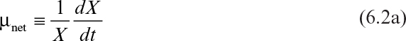
where X is cell mass concentration (g/l), t is time (h), and μnet is net specific growth rate (h–1). The net specific growth is the difference between a gross specific growth rate, μg (h–1), and the rate of loss of cell mass due to cell death or endogenous metabolism, kd (h–1).
Microbial growth can also be described in terms of cell number concentration, N, as well as X:

where μR is the net specific replication rate (h–1). If we ignore cell death, kd, then we use the symbol μ′R, and in cases where cell death is unimportant, μR will equal μ′R.
Similar to specific rate of growth, specific rates of substrate consumption (qs) and product formation (qp) can be defined as


where qs and qp are in units of g substrate/g biomass-h and g product/g biomass-h, respectively.
In this chapter, we discuss how the specific growth, substrate consumption, and product formation rates change with their environment. First, we consider growth in batch culture, where growth conditions are constantly changing.
6.1. Batch Growth
Batch growth refers to culturing cells in a vessel with an initial charge of medium that is not altered by further nutrient addition or removal. This form of cultivation is simple and widely used both in the laboratory and industrially.
6.1.1. Quantifying Cell Concentration
The quantification of cell concentration in a culture medium is essential for the determination of the kinetics and stoichiometry of microbial growth. The methods used in the quantification of cell concentration can be classified in two categories: direct and indirect. In many cases, the direct methods are not feasible because of the presence of suspended solids or other interfering compounds in the medium. Either cell number or cell mass can be quantified depending on the type of information needed and the properties of the system. Cell mass concentration is often preferred to the measurement of cell number density when only one is measured, but the combination of the two measurements is often desirable.
6.1.1.1. Determining cell number density.
A Petroff–Hausser counting chamber, or hemocytometer, is often used for direct cell counting. In this method, a calibrated grid is placed over the culture chamber, and the number of cells per grid square is counted using a microscope. To be statistically reliable, at least 20 grid squares must be counted and averaged. The culture medium should be clear and free of particles that could hide cells or be confused with cells. Stains can be used to distinguish between dead and live cells. This method is suitable for nonaggregated cultures. It is difficult to count molds under the microscope because of their mycelial nature.
Plates containing appropriate growth medium gelled with agar (Petri dishes) are used for counting viable cells. (The word viable used in this context means capable of reproduction.) Culture samples are diluted and spread on the agar surface and the plates are incubated. Colonies are counted on the agar surface following the incubation period. The results are expressed in terms of colony-forming units (CFU). If cells form aggregates, then a single colony may not be formed from a single cell. This method (plate counts) is more suitable for bacteria and yeasts and much less suitable for molds. A large number of colonies must be counted to yield a statistically reliable number. Growth media have to be selected carefully, since some media support growth better than others. The viable count may vary, depending on the composition of the growth medium. From a single cell, it may require 25 generations to form an easily observable colony. Unless the correct medium and culture conditions are chosen, some cells that are metabolically active may not form colonies.
In an alternative method, an agar–gel medium is placed in a small ring mounted on a microscope slide, and cells are spread on this miniature culture dish. After an incubation period of a few doubling times, the slide is examined with a microscope to count cells. This method has many of the same limitations as plate counts, but it is faster, and cells capable of only limited reproduction will be counted.
Another method is based on the relatively high electrical resistance of cells (Figure 6.1). Commercial particle counters employ two electrodes and an electrolyte solution. One electrode is placed in a tube containing an orifice. A vacuum is applied to the inner tube, which causes an electrolyte solution containing the cells to be sucked through the orifice. An electrical potential is applied across the electrodes. As cells pass through the orifice, the electrical resistance increases and causes pulses in electrical voltage. The number of pulses is a measure of the number of particles; particle concentration is known, since the counter is activated for a predetermined sample volume. The height of the pulse is a measure of cell size. Probes with various orifice sizes are used for different cell sizes. This method is suitable for discrete cells in a particulate-free medium and cannot be used for mycelial organisms.
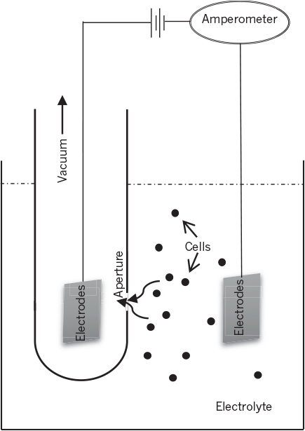
Figure 6.1. Schematic of a particle counter using the electrical resistance method to measure the cell number and cell size distribution.
The number of particles in solution can be determined from the measurement of scattered light intensity with the aid of a phototube (nephelometry). Light passes through the culture sample, and a phototube measures the light scattered by cells in the sample. The intensity of the scattered light is proportional to cell concentration. This method gives best results for dilute cell and particle suspensions.
6.1.1.2. Determining cell mass concentration.
Determination of cellular dry weight is the most commonly used direct method for determining cell mass concentration and is applicable only for cells grown in solids-free medium. If noncellular solids, such as molasses solids, cellulose, or corn steep liquor, are present, the dry weight measurement will be inaccurate. Typically, samples of culture broth are centrifuged or filtered and washed with a buffer solution or water. The washed wet cell mass is then dried at 80°C for 24 hours; then dry cell weight is measured.
Packed cell volume is used to rapidly but roughly estimate the cell concentration in a fermentation broth (e.g., industrial antibiotic fermentations). Fermentation broth is centrifuged in a tapered graduated tube under standard conditions (rpm and time), and the volume of cells is measured.
Another rapid method is based on the absorption of light by suspended cells in sample culture media. The intensity of the transmitted light is measured using a spectrometer. Turbidity or optical density measurement of the culture medium provides a fast, inexpensive, and simple method of estimating cell density in the absence of other solids or light-absorbing compounds. The extent of light transmission in a sample chamber is a function of cell density and the thickness of the chamber. Light transmission is modulated by both absorption and scattering. Pigmented cells give different results than unpigmented ones. Background absorption by components in the medium must be considered. The medium should be essentially particle free. Proper procedure entails using a wavelength that minimizes absorption by medium components (600 to 700 nm wavelengths are often used), “blanking” against medium, and using a calibration curve. The calibration curve relates optical density (OD) to dry-weight measurements. Such calibration curves can become nonlinear at high OD values (>0.3) and depend to some extent on the physiological state of the cells.
In many fermentation processes, such as mold fermentations, direct methods cannot be used. In such cases, indirect methods are used, which are based mainly on the measurement of substrate consumption and/or product formation during the course of growth.
Intracellular components of cells such as RNA, DNA, and protein can be measured as indirect measures of cell growth. During a batch growth cycle, the concentrations of these intracellular components change with time. Figure 6.2 depicts the variation of certain intracellular components with time during a batch growth cycle. Concentration of RNA (RNA/cell weight) varies significantly during a batch growth cycle; however, DNA and protein concentrations remain fairly constant. Therefore, in a complex medium, DNA concentration can be used as a measure of microbial growth. Cellular protein measurements can be achieved using different methods. Total amino acids, Biuret, Lowry (Folin reagent), and Kjeldahl nitrogen measurements can be used for this purpose. Total amino acids and the Lowry method are the most reliable. Recently, protein determination kits from several vendors have been developed for simple and rapid protein measurements. However, many media contain proteins as substrates, which limits the usefulness of this approach.

Figure 6.2. Time-dependent changes in cell composition and cell size for Azotobacter vinelandii in batch culture. (With permission, from M. L. Shuler and H. M. Tsuchiya, “Cell Size as an Indicator of Changes in Intracellular Composition of Azotobacter vinelandii,” Canadian Journal of Microbiology, 1975, 21(6): 927–935, National Research Council of Canada, Ottawa. © Canadian Science Publishing or its licensors.)
The intracellular adenosine triphosphate (ATP) concentration (mg ATP/mg cells) is approximately constant for a given organism. Thus, the ATP concentration in a fermentation broth can be used as a measure of biomass concentration. The method is based on luciferase activity, which catalyzes oxidation of luciferin at the expense of oxygen and ATP with the emission of light:
When oxygen and luciferin are in excess, total light emission is proportional to total ATP present in the sample. Photometers can be used to detect emitted light. Small concentrations of biomass can be measured by this method, since very low concentrations of ATP (10–12 g ATP/l) can be measured by photometers or scintillation counters. The ATP content of a typical bacterial cell is 1 mg ATP/g dry-weight cell, approximately.
Sometimes, nutrients used for cellular mass production can be measured to follow microbial growth. Nutrients used for product formation are not suitable for this purpose. Nitrate, phosphate, or sulfate measurements can be used. The utilization of a carbon source or oxygen uptake rate can be measured to monitor cellular growth when cell mass is the major product.
The products of cell metabolism can be used to monitor and quantify cellular growth. Certain products produced under anaerobic conditions, such as ethanol and lactic acid, can be related nearly stoichiometrically to microbial growth. Products must be either growth associated (ethanol) or mixed growth associated (lactic acid) to be correlated with microbial growth. For aerobic fermentations, CO2 is a common product and can be related to microbial growth. In some cases, changes in the pH or acid–base addition to control pH can be used to monitor nutrient uptake and microbial growth. For example, the utilization of ammonium results in the release of hydrogen ions (H+) and therefore a drop in pH. The amount of base added to neutralize the H+ released is proportional to ammonium uptake and growth. Similarly, when nitrate is used as the nitrogen source, hydrogen ions are removed from the medium, resulting in an increase in pH. In this case, the amount of acid added is proportional to nitrate uptake and therefore to microbial growth.
In some fermentation processes, as a result of mycelial growth or extracellular polysaccharide formation, the viscosity of the fermentation broth increases during the course of fermentation. If the substrate is a biodegradable polymer, such as starch or cellulose, then the viscosity of the broth decreases with time as biohydrolysis continues. Changes in the viscosity of the fermentation broth can be correlated with the extent of microbial growth. Although polymeric broths are usually non-Newtonian, the apparent viscosity measured at a fixed rate can be used to estimate cell or product concentration.
6.1.2. Growth Patterns and Kinetics in Batch Culture
When a liquid nutrient medium is inoculated with a seed culture, the organisms selectively take up dissolved nutrients from the medium and convert them into biomass. A typical batch growth curve includes the following phases: lag phase, logarithmic or exponential growth phase, deceleration phase, stationary phase, and death phase. Figure 6.3 describes a batch growth cycle.
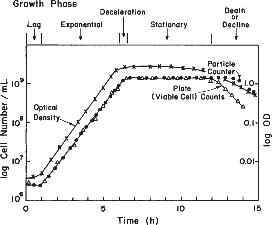
Figure 6.3. Typical growth curve for a bacterial population. Note that the phase of growth (shown here for cell number) depends on the parameter used to monitor growth.
The lag phase occurs immediately after inoculation and is a period of adaptation of cells to a new environment. Microorganisms reorganize their molecular constituents when they are transferred to a new medium. Depending on the composition of nutrients, new enzymes are synthesized, the synthesis of some other enzymes is repressed, and the internal machinery of cells is adapted to the new environmental conditions. These changes reflect the intracellular mechanisms for the regulation of the metabolic processes discussed in Chapter 4, “How Cells Work.” During this phase, cell mass may increase a little, without an increase in cell number density. When the inoculum is small and has a low fraction of cells that are viable, there may be a pseudolag phase, which is a result not of adaptation but of small inoculum size or poor condition of the inoculum.
Low concentration of some nutrients and growth factors may also cause a long lag phase. For example, the lag phase of Enterobacter aerogenes (formerly Aerobacter aerogenes) grown in glucose and phosphate buffer medium increases as the concentration of Mg2+, which is an activator of the enzyme phosphatase, is decreased. As another example, even heterotrophic cells require CO2 fixation (to supplement intermediates removed from key energy-producing metabolic cycles during rapid biosynthesis), and excessive sparging can remove metabolically generated CO2 too rapidly for cellular restructuring to be accomplished efficiently, particularly with a small inoculum.
The age of the inoculum culture has a strong effect on the length of lag phase. The age refers to how long a culture has been maintained in a batch culture. Usually, the lag period increases with the age of the inoculum. In some cases, there is an optimal inoculum age resulting in minimum lag period. To minimize the duration of the lag phase, cells should be adapted to the growth medium and conditions before inoculation, and cells should be young (or exponential phase cells) and active, and the inoculum size should be large (5% to 10% by volume). The nutrient medium may need to be optimized and certain growth factors included to minimize the lag phase. Figure 6.4 shows an example of variation of the lag phase with MgSO4 concentration. Many commercial fermentation plants rely on batch culture; to obtain high productivity from a fixed plant size, the lag phase must be as short as possible.

Figure 6.4. Influence of Mg2+ concentration on the lag phase in E. aerogenes culture. (With permission, from A. C. R. Dean, C. Hinshelwood, Growth, Function, and Regulation in Bacterial Cells. Oxford Press, London, 1966, p. 55.)
Multiple lag phases may be observed when the medium contains more than one carbon source. This phenomenon, known as diauxic growth, is caused by a shift in metabolic pathways in the middle of a growth cycle (see Example 4.1). After one carbon source is exhausted, the cells adapt their metabolic activities to utilize the second carbon source. The first carbon source is more readily utilizable than the second, and the presence of more readily available carbon source represses the synthesis of the enzymes required for the metabolism of the second substrate.
The exponential growth phase is also known as the logarithmic growth phase. In this phase, the cells have adjusted to their new environment. After this adaptation period, cells can multiply rapidly, and cell mass and cell number density increase exponentially with time. This is a period of balanced growth in which all components of a cell grow at the same rate. That is, the average composition of a single cell remains approximately constant during this phase of growth. During balanced growth, the net specific growth rate determined from either cell number or cell mass would be the same. Since the nutrient concentrations are large in this phase, the growth rate is independent of nutrient concentration. The exponential growth rate is first order:

Integration of equation 6.7 yields

where X and X0 are cell concentrations at time t and t = 0.
The time required to double the microbial mass is given by equation 6.9. The exponential growth is characterized by a straight line on a semilogarithm plot of Ln X versus time, where τd is the doubling time of cell mass:

Similarly, we can calculate a doubling time based on cell numbers and the net specific rate of replication:

where τ′d is the doubling time based on the replication rate. During balanced growth, τd will equal τ′d, since the average cell composition and size will not change with time.
The deceleration growth phase follows the exponential phase. In this phase, growth decelerates due to either depletion of one or more essential nutrients or the accumulation of toxic by-products of growth. For a typical bacterial culture, these changes occur over a very short period of time. The rapidly changing environment results in unbalanced growth. During unbalanced growth, cell composition and size will change and τd and τ′d will not be equal. In the exponential phase, the cellular metabolic control system is set to achieve maximum rates of reproduction. In the deceleration phase, the stresses induced by nutrient depletion or waste accumulation cause a restructuring of the cell to increase the prospects of cellular survival in a hostile environment. These observable changes are the result of the molecular mechanisms of repression and induction that we discussed in Chapter 4. Because of the rapidity of these changes, cell physiology under conditions of nutrient limitation is more easily studied in continuous culture, as discussed later in this chapter.
The stationary phase starts at the end of the deceleration phase, when the net growth rate is zero (no cell division) or when the growth rate is equal to the death rate. Even though the net growth rate is zero during the stationary phase, cells are still metabolically active and produce secondary metabolites. Primary metabolites are growth-related products and secondary metabolites are nongrowth-related. In fact, the production of certain metabolites (e.g., antibiotics, some hormones) is enhanced during the stationary phase due to metabolite deregulation. During the course of the stationary phase, one or more of the following phenomena may take place:
• Total cell mass concentration may stay constant, but the number of viable cells may decrease.
• Cell lysis may occur and viable cell mass may drop. A second growth phase may occur and cells may grow on lysis products of lysed cells (cryptic growth).
• Cells may not be growing but may have active metabolism to produce secondary metabolites. Cellular regulation changes when concentrations of certain metabolites (carbon, nitrogen, phosphate) are low. Secondary metabolites are produced as a result of metabolite deregulation.
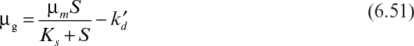
During the stationary phase, the cell catabolizes cellular reserves for new building blocks and for energy-producing monomers. This is called endogenous metabolism. The cell must always expend energy to maintain an energized membrane (i.e., proton-motive force) and transport of nutrients and for essential metabolic functions such as motility and repair of damage to cellular structures. This energy expenditure is called maintenance energy. The appropriate equation describing catabolism of cellular mass for maintenance energy or the loss of cell mass due to cell lysis during the stationary phase is

where kd is a first-order rate constant for endogenous metabolism, and Xso is the cell mass concentration at the beginning of the stationary phase. Because S is zero, μg is zero in the stationary phase.
The reason for termination of growth may be either exhaustion of an essential nutrient or accumulation of toxic products. If an inhibitory product is produced and accumulates in the medium, the growth rate will slow down, depending on inhibitor production, and at a certain level of inhibitor concentration, growth will stop. Ethanol production by yeast is an example of a fermentation in which the product is inhibitory to growth. Dilution of toxified medium, addition of an unmetabolizable chemical compound complexing with the toxin, or simultaneous removal of the toxin would alleviate the adverse effects of the toxin and yield further growth.
The death phase (or decline phase) follows the stationary phase. However, some cell death may start during the stationary phase, and a clear demarcation between these two phases is not always possible. Often, dead cells lyse, and intracellular nutrients released into the medium are used by the living organisms during the stationary phase. At the end of the stationary phase, because of either nutrient depletion or toxic product accumulation, the death phase begins.
The rate of death usually follows first-order kinetics:

where Ns is the concentration of cells at the end of the stationary phase and k′d is the first-order death-rate constant. A plot of Ln N versus t yields a line of slope –k′d. During the death phase, cells may or may not lyse, and the reestablishment of the culture may be possible in the early death phase if cells are transferred into a nutrient-rich medium. In both the death and stationary phases, it is important to recognize that there is a distribution of properties among individuals in a population. With a narrow distribution, cell death will occur nearly simultaneously; with a broad distribution, a subfraction of the population may survive for an extended period. It is this subfraction that would dominate the reestablishment of a culture from inoculum derived from stationary or death-phase cultures. Thus, using an old inoculum may select for variants of the original strain having altered metabolic capabilities.
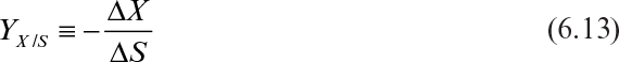
To better describe growth kinetics, we define some stoichiometrically related parameters. Yield coefficients are defined on the basis of the amount of consumption of another material. For example, the growth yield coefficient in fermentation is
At the end of the batch growth period, we have an apparent growth yield (or observed growth yield). Because culture conditions can alter patterns of substrate utilization, the apparent growth yield is not a true constant.
The consumption of a substrate for chemoheterotrophic growth is used to supply both energy and carbon as a building block for the synthesis of cellular components. There is also the concept of maintenance. Maintenance was first described as energy consumed for functions other than production of new cell material, but these “nongrowth” uses of substrate are complex and context dependent (see van Bodegom† for a more complete description). We will adapt a fairly standard approach to the description of these components, but understand that there are many subtitles to these concepts.
† P. van Bodegom, “Microbial Maintenance: A Critical Review on Its Quantification,” Microbial Ecology 53(4): 513–523, 2007.
If we take as an example the consumption of a sugar (such as glucose) in a simple chemically defined medium, we can summarize the use of the glucose as follows:
Equation 6.14 summarizes the major ways glucose is utilized. The first is to use glucose to make cellular components such as DNA, RNA, proteins, polysaccharides, and other small carbon-containing molecules. In addition to these intracellular components, glucose supplies the carbon for extracellular products, such as proteins made from recombinant DNA techniques. The term ∆Sgrowth energy denotes the glucose consumed to generate energy, typically in the form of ATP or GTP (guanosine triphosphate), which is then used in biosynthesis of macromolecules and transport of substrates in or product out of the cell and other growth-related functions. ∆Smaintenance energy refers to substrate consumed to produce ATP or GTP to sustain the cell for nongrowth-related functions such as repair of damaged cellular components, osmotic pressure balancing, motility, defense against O2 stress, and energy-spilling reactions. The breakdown of glucose to supply energy may result in the formation of CO2 due to oxygen consumption (aerobic) or due to formation of a partially oxidized compound such as ethanol and CO2 (anaerobic). Such compounds (e.g., ethanol and CO2) are also “products” from the breakdown of glucose, and indeed, as shown in Chapter 5, “Major Metabolic Pathways,” many are important commercial products.
In Section 6.3, we differentiate between the true (or maximum) growth yield, which is constant, and the apparent yield. Yield coefficients based on other substrates or product formation may be defined as

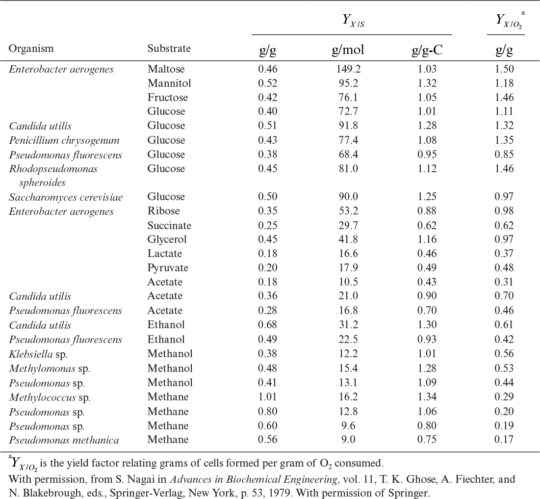
For organisms growing aerobically on glucose, YX/S is typically 0.4 to 0.6 g/g for most yeast and bacteria, while YO2 is 0.9 to 1.4 g/g. Anaerobic growth is less efficient, and the yield coefficient is reduced substantially (see Figure 6.5). With substrates that are more or less reduced than glucose, the value of the apparent yield coefficient will change. For methane, YX/S would assume values of 0.6 to 1.0 g/g, with the corresponding YX/O2 decreasing to about 0.2 g/g. In most cases, the yield of biomass on a carbon-energy source is 1.0 ± 0.4 g biomass per g of carbon consumed. Table 6.1 lists some examples of YX/S and YX/O2 for a variety of substrates and organisms.
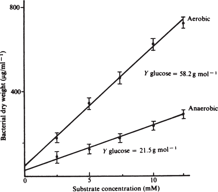
Figure 6.5. Aerobic and anaerobic growth yields of Streptococcus faecalis with glucose as substrate. (B. Atkinson and F. Mavituna, Biochemical Engineering and Biotechnology Handbook, Macmillan, Inc., New York, 1983. Reproduced with permission of Palgrave Macmillan.)
Two closely linked parameters are often used to describe nongrowth-related functions. There are difficulties in employing these parameters and disagreement among authors. These nongrowth functions are most easily observed and discussed in terms of continuous culture, which is described in Section 6.3. The maintenance coefficient, m, is often defined as

where (dS/dt)m represents the consumption of substrate for maintenance functions. Given the complexity of what is included in maintenance and the conceptual difficulty of applying the concept to a simple model in which there is no explicit accounting of the internal structure of the cell, the term (dS/dt)m should be viewed as a bookkeeping term.
Depending on the culture conditions, maintenance may be largely due to endogenous metabolism (although some nongrowth functions are not included in endogenous metabolism but are included in maintenance). When substrate and energy are present in large amounts, maintenance and endogenous metabolism are quantitatively small terms, whereas in stationary growth, when external substrate is present at a low level, endogenous metabolism dominates. Endogenous metabolism consists of the breakdown of cellular compounds such as polysaccharides, but also proteins and RNA, for monomers to make new macromolecules and for energy for cellular function. The term kd in equation 6.11 is the rate constant for endogenous metabolism.
Microbial growth, product formation, and substrate utilization rates are usually expressed in the form of specific rates (e.g., normalized with respect to X), since bioreactions are autocatalytic. The specific rates are used to compare the effectiveness of various fermentation schemes and biocatalysts.
Microbial products can be classified in three major categories (see Figure 6.6):
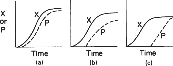
Figure 6.6. Kinetic patterns of growth and product formation in batch fermentations: (a) growth-associated product formation, (b) mixed-growth-associated product formation, and (c) nongrowth-associated product formation.
• Growth-associated products are produced simultaneously with microbial growth. The specific rate of product formation is proportional to the specific rate of growth, μg. Note that μg differs from μnet, the net specific growth rate, when endogenous metabolism is nonzero:

The production of a constitutive enzyme is an example of a growth-associated product.
• Nongrowth-associated product formation takes place during the stationary phase when the growth rate is zero. The specific rate of product formation is constant:
Many secondary metabolites, such as antibiotics (e.g., penicillin), are nongrowth-associated products.
• Mixed-growth-associated product formation takes place during the slow growth and stationary phases. In this case, the specific rate of product formation is given by the following equation:
Lactic acid fermentation, xanthan gum, and some secondary metabolites from cell culture are examples of mixed-growth-associated products. Equation 6.20 is a Luedeking–Piret equation. If α = 0, the product is only nongrowth associated, and if β = 0, the product would be only growth associated, and consequently α would be equal to YP/X.
Some of the concepts concerning growth rate and yield are illustrated in Example 6.1.
Example 6.1 Calculation of Growth Parameters
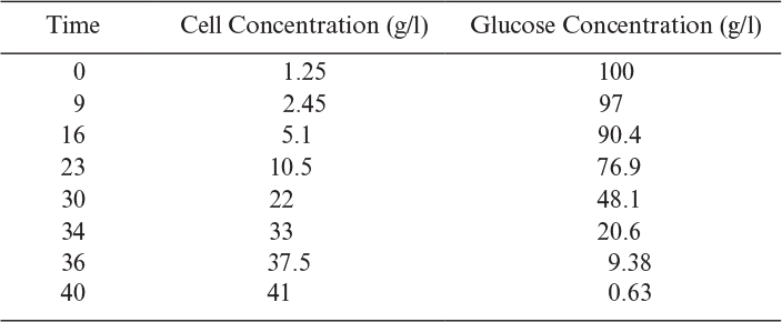
a. Calculate the maximum net specific growth rate.
b. Calculate the apparent growth yield.
c. What maximum cell concentration could one expect if 150 g of glucose were used with the same size inoculum?
a. 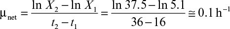
b. 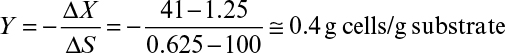
c. ![]()
6.1.3. How Environmental Conditions Affect Growth Kinetics
The patterns of microbial growth and product formation we have just discussed are influenced by environmental conditions such as temperature, pH, and dissolved-oxygen concentration.
Temperature is an important factor affecting the performance of cells. According to their temperature optima, organisms can be classified in three groups: psychrophiles (Topt < 20°C), mesophiles (Topt = from 20° to 50°C), and thermophiles (Topt > 50°C). As the temperature is increased toward optimal growth temperature, the growth rate approximately doubles for every 10°C increase in temperature. Above the optimal temperature range, the growth rate decreases and thermal death may occur. The net specific replication rate for temperature above optimal level can be expressed by

At high temperatures, the thermal death rate exceeds the growth rate, which causes a net decrease in the concentration of viable cells.
Both ![]() and
and ![]() vary with temperature according to the Arrhenius equation:
vary with temperature according to the Arrhenius equation:
where Ea and Ed are activation energies for growth and thermal death. The activation energy for growth is typically 10 to 20 kcal/mol, and for thermal death, 60 to 80 kcal/mol. That is, thermal death is more sensitive to temperature changes than microbial growth.
Temperature also affects product formation. However, the temperature optimum for growth and product formation may be different. The yield coefficient is also affected by temperature. In some cases, such as single-cell protein production, temperature optimization to maximize the yield coefficient (YX/S) is critical. When temperature is increased above the optimum temperature, the maintenance requirements of cells increase. That is, the maintenance coefficient (see equation 6.17) increases with increasing temperature with an activation energy of 15 to 20 kcal/mol, resulting in a decrease in the yield coefficient.
Temperature also may affect the rate-limiting step in a fermentation process. At high temperatures, the rate of bioreaction might become higher than the diffusion rate, and diffusion would then become the rate-limiting step (e.g., in an immobilized cell system). The activation energy of molecular diffusion is about 6 kcal/mol. The activation energy for most bioreactions is more than 10 kcal/mol, so diffusional limitations must be carefully considered at high temperatures. Figure 6.7 depicts a typical variation of growth rate with temperature.

Figure 6.7. Arrhenius plot of growth rate of Escherichia coli B/r. Individual data points are marked with corresponding degrees Celsius. E. coli B/r was grown in a rich complex medium (![]() ) and a glucose-mineral salts medium (○). (After S. L. Herendeen, R. A. VanBogelen, F. C. Neidhardt, “Levels of Major Protein of Escherichia coli during Growth at Different Temperatures,” J. Bacteriol. 139:195, 1979, as drawn in R. Y. Stanier and others, The Microbial World, 5th ed., Pearson Education, Upper Saddle River, NJ, 1986, p. 207.)
) and a glucose-mineral salts medium (○). (After S. L. Herendeen, R. A. VanBogelen, F. C. Neidhardt, “Levels of Major Protein of Escherichia coli during Growth at Different Temperatures,” J. Bacteriol. 139:195, 1979, as drawn in R. Y. Stanier and others, The Microbial World, 5th ed., Pearson Education, Upper Saddle River, NJ, 1986, p. 207.)
Hydrogen-ion concentration (pH) affects the activity of enzymes and therefore the microbial growth rate. The optimal pH for growth may be different from that for product formation. Generally, the acceptable pH range varies about the optimum by ±1 to 2 pH units. Different organisms have different pH optima: the pH optimum for many bacteria ranges from pH = 3 to 8; for yeast, pH = 3 to 6; for molds, pH = 3 to 7; for plant cells, pH = 5 to 6; and for animal cells, pH = 6.5 to 7.5. Many organisms have mechanisms to maintain intracellular pH at a relatively constant level in the presence of fluctuations in environmental pH. When pH differs from the optimal value, the maintenance-energy requirements increase. One consequence of different pH optima is that the pH of the medium can be used to select one organism over another.
In most fermentations, pH can vary substantially. Often, the nature of the nitrogen source can be important. If ammonium is the sole nitrogen source, hydrogen ions are released into the medium as a result of the microbial utilization of ammonia, resulting in a decrease in pH. If nitrate is the sole nitrogen source, hydrogen ions are removed from the medium to reduce nitrate to ammonia, resulting in an increase in pH. Also, pH can change because of the production of organic acids, the utilization of acids (particularly amino acids), or the production of bases. The evolution or supply of CO2 can alter pH greatly in some systems (e.g., seawater or animal cell culture). Thus, pH control by means of a buffer or an active pH control system is important. Variation of specific growth rate with pH is depicted in Figure 6.8, indicating a pH optimum.

Figure 6.8. Typical variation of specific growth rate with pH. The units are arbitrary. With some microbial cultures, it is possible to adapt cultures to a wider range of pH values if pH changes are made in small increments from culture transfer to transfer.
Dissolved oxygen (DO) is an important substrate in aerobic fermentations and may be a limiting substrate, since oxygen gas is sparingly soluble in water. At high cell concentrations, the rate of oxygen consumption may exceed the rate of oxygen supply, leading to oxygen limitations. When oxygen is the rate-limiting factor, specific growth rate varies with DO concentration according to saturation kinetics; below a critical concentration, growth or respiration approaches a first-order rate dependence on the DO concentration.
Above a critical oxygen concentration, the growth rate becomes independent of the DO concentration. Figure 6.9 depicts the variation of specific growth rate with DO concentration. Oxygen is a growth-rate-limiting factor when the DO level is below the critical DO concentration. In this case, another medium component (e.g., glucose, ammonium) becomes growth-extent limiting. For example, with Azotobacter vinelandii at a DO = 0.05 mg/l, the growth rate is about 50% of maximum even if a large amount of glucose is present. However, the maximum amount of cells formed is not determined by the DO, as oxygen is continually resupplied. If glucose were totally consumed, growth would cease even if DO = 0.05 mg/l. Thus, the extent of growth (mass of cells formed) would depend on glucose, while the growth rate for most of the culture period would depend on the value of DO.
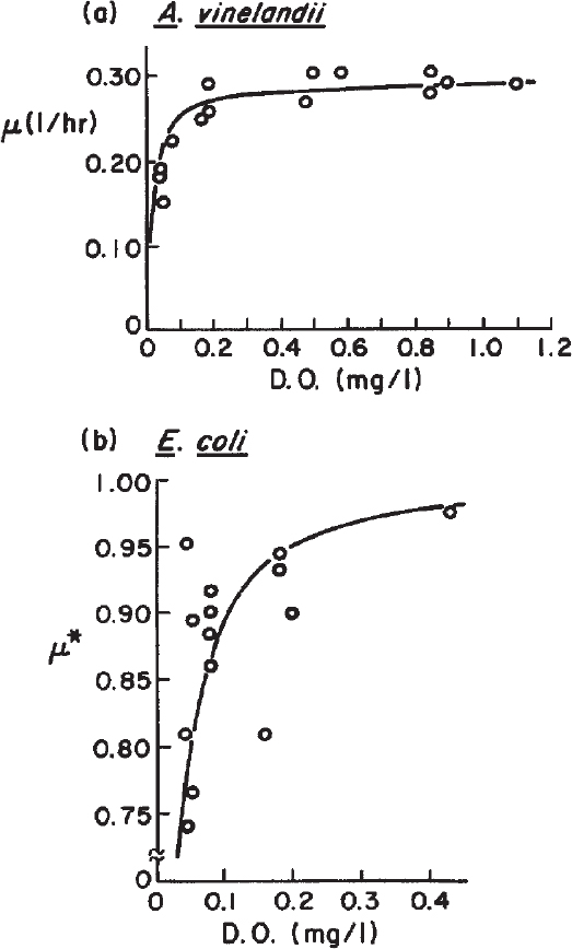
Figure 6.9. Growth-rate dependence on dissolved oxygen for (a) Azotobacter vinelandii, a strictly aerobic organism, and (b) Escherichia coli, which is facultative. E. coli grows anaerobically at a rate of about 70% of its aerobic growth in minimal medium. Note that μ* is defined as follows: ![]()
The critical oxygen concentration is about 5% to 10% of the saturated DO concentration for bacteria and yeast and about 10% to 50% of the saturated DO concentration for mold cultures, depending on the pellet size of molds. Saturated DO concentration in water at 25°C and 1 atm pressure is about 7 ppm. The presence of dissolved salts and organics can alter the saturation value, whereas increasingly high temperatures decrease the saturation value.
Oxygen is usually introduced to fermentation broth by sparging air through the broth. Oxygen transfer from gas bubbles to cells is usually limited by oxygen transfer through the liquid film surrounding the gas bubbles. The rate of oxygen transfer from the gas to liquid phase is given by
where kL is the oxygen transfer coefficient (cm/h), a is the gas–liquid interfacial area (cm2/cm3), kLa is the volumetric oxygen transfer coefficient (h–1), C* is saturated DO concentration (mg/1), CL is the actual DO concentration in the broth (mg/1), and No2 is the rate of oxygen transfer (mg O2/l-h). Also, the term oxygen transfer rate (OTR) is used.
The rate of oxygen uptake is denoted as OUR (oxygen uptake rate) and when maintenance can be neglected is given by equation 6.24:

where qO2 is the specific rate of oxygen consumption (mg O2/g dw cells-h), YX/O2 is the yield coefficient on oxygen (g dw cells/g O2), and X is cell concentration (g dw cells/1).
When oxygen transfer is the rate-limiting step, the rate of oxygen consumption is equal to the rate of oxygen transfer. If the maintenance requirement of O2 is negligible compared to growth, then we get
or

Growth rate varies nearly linearly with the OTR under oxygen-transfer limitations. Among the various methods used to overcome DO limitations are the use of oxygen-enriched air or pure oxygen and operation under high atmospheric pressure (2 to 3 atm). Oxygen transfer has a big impact on reactor design (see Chapter 10, “Selection, Scale-Up, Operation, and Control of Bioreactors”).
The redox potential is an important parameter that affects the rate and extent of many oxidative–reductive reactions. In a fermentation medium, the redox potential is a complex function of DO, pH, and other ion concentrations, such as reducing and oxidizing agents. The electrochemical potential of a fermentation medium can be expressed by

The electrochemical potential is measured in millivolts by a pH/voltmeter, and Po2 is in atmospheres.
The redox potential of a fermentation medium can be reduced by passing nitrogen gas or by the addition of reducing agents such as cysteine HCl or Na2S. Oxygen gas can be passed or some oxidizing agents can be added to the fermentation medium to increase the redox potential.
Dissolved carbon dioxide (DCO2) concentration may have a profound effect on performance of organisms. Very high DCO2 concentrations may be toxic to some cells. However, cells require a certain DCO2 level for proper metabolic functions. The dissolved carbon dioxide concentration can be controlled by changing the CO2 content of the air supply and the agitation speed.
The ionic strength of the fermentation medium affects the transport of certain nutrients into and out of cells, the metabolic functions of cells, and the solubility of certain nutrients, such as DO. The ionic strength is given by
where C is the concentration of an ion, Zi is its charge, and I is the ionic strength of the medium.
High substrate concentrations that are significantly above stoichiometric requirements are inhibitory to cellular functions. Inhibitory levels of substrates vary depending on the type of cells and substrate. Glucose may be inhibitory at concentrations above 200 g/l (e.g., ethanol fermentation by yeast), probably due to a reduction in water activity. Certain salts, such as NaCl, may be inhibitory at concentrations above 40 g/l due to high osmotic pressure. Some refractory compounds, such as phenol, toluene, and methanol, are inhibitory at much lower concentrations (e.g., 1 g/l). Typical maximum noninhibitory concentrations of some nutrients are glucose, 100 g/l; ethanol, 50 g/l for yeast, much less for most organisms; ammonium, 5 g/l; phosphate, 10 g/l; and nitrate, 5 g/l. Substrate inhibition can be overcome by intermittent addition of the substrate to the medium.
6.1.4. Heat Generation by Microbial Growth
About 40% to 50% of the energy stored in a carbon and energy source is converted to biological energy (ATP) during aerobic metabolism, and the rest of the energy is released as heat. For actively growing cells, the maintenance requirement is low, and heat evolution is directly related to growth.
The heat generated during microbial growth can be calculated using the heat of combustion of the substrate and of cellular material. A schematic of an enthalpy balance for microbial utilization of substrate is presented in Figure 6.10. The heat of combustion of the substrate is equal to the sum of the metabolic heat and the heat of combustion of the cellular material:

where ∆Hs is the heat of combustion of the substrate (kJ/g substrate), YX/S is the substrate yield coefficient (g cell/g substrate), ∆Hc is the heat of combustion of cells (kJ/g cells), and 1/YH is the metabolic heat evolved per gram of cell mass produced (kJ/g cells).
Equation 6.29a can be rearranged to yield
∆Hs and ∆Hc can be determined from the combustion of substrate and cells. Typical ∆Hc values for bacterial cells are 20 to 25 kJ/g cells. Typical values of YH are glucose, 0.42 g/kcal; malate, 0.30 g/kcal; acetate, 0.21 g/kcal; ethanol, 0.18 g/kcal; methanol, 0.12 g/kcal; and methane, 0.061 g/kcal. Clearly, the degree of oxidation of the substrate has a strong effect on the amount of heat released. The total rate of heat evolution in a batch fermentation is
where VL is the liquid volume (l) and X is the cell concentration (g/l).
In aerobic fermentations, the rate of metabolic heat evolution can roughly be correlated to the rate of oxygen uptake, since oxygen is the final electron acceptor:
where QGR is in units of kcal/h, and Qo2 is in millimoles of O2/h.
Metabolic heat released during fermentation can be removed by circulating cooling water through a cooling coil or cooling jacket in the fermenter. Often, temperature control (adequate heat removal) is an important limitation on reactor design (see Chapter 10). The ability to estimate heat-removal requirements is essential to proper reactor design.
6.2. Quantifying Growth Kinetics
In the previous section, we described some key concepts in the growth of cultures. Clearly, we can think of the growth dynamics in terms of kinetic descriptions. It is essential to recall that cellular composition and biosynthetic capabilities change in response to new growth conditions (unbalanced growth), although a constant cellular composition and balanced growth can predominate in the exponential growth phase. If the decelerating growth phase is due to substrate depletion rather than inhibition by toxins, the growth rate decreases in relation to decreasing substrate concentrations. In the stationary and death phases, the distribution of properties among individuals is important (e.g., cryptic death). Although these kinetic ideas are evident in batch culture, they are equally evident and important in other modes of culture (e.g., continuous culture).
The complete description of the growth kinetics of a culture would involve recognition of the structured nature of each cell and the segregation of the culture into individual units (cells) that may differ from each other. Models can have these same attributes. A chemically structured model divides the cell mass into components. If the ratio of these components can change in response to perturbations in the extracellular environment, then the model is behaving analogously to a cell changing its composition in response to environmental changes. Consider in Chapter 4, “How Cells Work,” our discussion of cellular regulation, particularly the induction of whole pathways. Any of these metabolic responses results in changes in intracellular structure. Furthermore, if a model of a culture is constructed from discrete units, it begins to mimic the segregation observed in real cultures. Models may be structured and segregated, structured and nonsegregated, unstructured and segregated, or unstructured and nonsegregated. Models containing both structure and segregation are the most realistic, but they are also computationally complex.
The degree of realism and complexity required in a model depends on what is being described; the modeler should always choose the simplest model that can adequately describe the desired system. An unstructured model assumes fixed cell composition, which is equivalent to assuming balanced growth. The balanced-growth assumption is valid primarily in single-stage, steady-state continuous culture and the exponential phase of batch culture; it fails during any transient condition. How fast the cell responds to perturbations in its environment and how fast these perturbations occur determine whether pseudobalanced growth can be assumed. If cell response is fast compared to external changes and if the magnitude of these changes is not too large (e.g., a 10% or 20% variation from initial conditions), then the use of unstructured models can be justified, since the deviation from balanced growth may be small. Culture response to large or rapid perturbations cannot be described satisfactorily by unstructured models.
For many systems, segregation is not a critical component of culture response, so nonsegregated models will be satisfactory under many circumstances. An important exception is the prediction of the growth responses of plasmid-containing cultures (see Chapter 14, “Utilizing Genetically Engineered Organisms”).
Because of the introductory nature of this book, we will concentrate our discussion on unstructured and nonsegregated models. Be aware of the limitations on these models. Nonetheless, such models are simple and applicable to some situations of practical interest.
6.2.1. Unstructured Nonsegregated Models
The simplest models are unstructured, nonsegregated models, but they can be powerful. Primarily, they are effective at predicting specific growth as a function of substrate concentrations. They also can be extended to predict response to a variety of inhibitors or activators. They can be applied not only to bacteria but also to filamentous organisms. These models are useful in the design of bioreactors.
6.2.1.1. Substrate-limited growth.
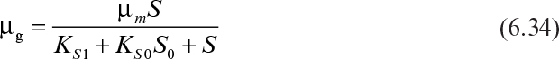
As shown in Figure 6.11, the relationship of specific growth rate to substrate concentration often assumes the form of saturation kinetics. Here we assume that a single chemical species, S, is growth-rate limiting (i.e., an increase in S influences growth rate, while changes in other nutrient concentrations have no effect). These kinetics are similar to the Langmuir–Hinshelwood (or Hougen–Watson) kinetics in traditional chemical kinetics or Michaelis–Menten kinetics for enzyme reactions. When applied to cellular systems, these kinetics can be described by the Monod equation:
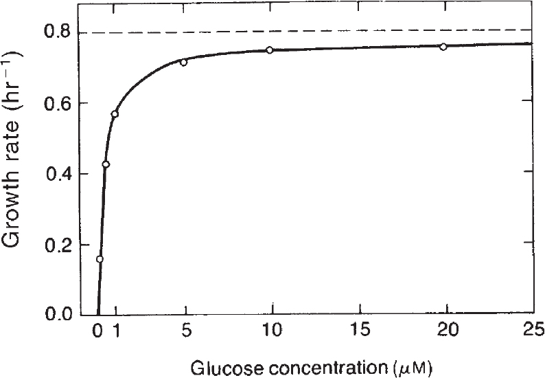
Figure 6.11. Effect of nutrient concentration on the specific growth rate of Escherichia coli. (R. Y. Stainer, J. L. Ingraham, M. L. Wheelis, P. R. Painter, The Microbial World, 5th ed., © 1986. Reprinted and electronically reproduced by permission of Pearson Education, Inc., New York, NY.)
where μm is the maximum specific growth rate when S >> Ks. If endogenous metabolism is unimportant, then μnet = μg. The constant Ks is known as the saturation constant or half-velocity constant and is equal to the concentration of the rate-limiting substrate when the specific rate of growth is equal to one-half of the maximum. That is, Ks = S when μg = ![]() μmax In general, μg = μm for S >> Ks, and μg = (μm/Ks)S for S << Ks. The Monod equation is semiempirical; it derives from the premise that a single-enzyme system with Michaelis–Menten kinetics is responsible for uptake of S, and the amount of that enzyme or its catalytic activity is sufficiently low to be growth-rate limiting.
μmax In general, μg = μm for S >> Ks, and μg = (μm/Ks)S for S << Ks. The Monod equation is semiempirical; it derives from the premise that a single-enzyme system with Michaelis–Menten kinetics is responsible for uptake of S, and the amount of that enzyme or its catalytic activity is sufficiently low to be growth-rate limiting.
This simple premise is rarely, if ever, true; however, the Monod equation empirically fits a wide range of data satisfactorily and is the most commonly applied unstructured, nonsegregated model of microbial growth.
The Monod equation describes substrate-limited growth only when growth is slow and population density is low. Under these circumstances, environmental conditions can be related simply to S. If the consumption of a carbon–energy substrate is rapid, then the release of toxic waste products is more likely (due to energy-spilling reactions). At high population levels, the buildup of toxic metabolic by-products becomes more important. The following rate expressions have been proposed for rapidly growing dense cultures:

or
where S0 is the initial concentration of the substrate and KS0 is dimensionless.
Other equations have been proposed to describe the substrate-limited growth phase. Depending on the shape of the μ–S curve, one of these equations may be more plausible than the others. The following equations are alternatives to the Monod equation:
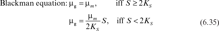


Although the Blackman equation often fits the data better than the Monod equation, the discontinuity in the Blackman equation is troublesome in many applications. The Tessier equation has two constants (μm, K), and the Moser equation has three constants (μm, KS, n). The Moser equation is the most general form of these equations, and it is equivalent to the Monod equation when n = 1. The Contois equation has a saturation constant proportional to cell concentration that describes substrate-limited growth at high cell densities. According to this equation, the specific growth rate decreases with decreasing substrate concentrations and eventually becomes inversely proportional to the cell concentration in the medium (i.e., μg ∞ X–1).
These equations can be described by a single differential equation:

where υ = μg/μm, S is the rate-limiting substrate concentration, and K, a, and b are constants. The values of these constants are different for each equation and are listed in Table 6.2.

TABLE 6.2. Constants of the Generalized Differential Specific Growth Rate Equation 6.39 for Different Models
The correct rate form to use when more than one substrate is potentially growth-rate limiting is an unresolved question. However, under most circumstances, the noninteractive approach works best:
The lowest value of μg(Si) is used.
6.2.1.2. Models with growth inhibitors.
At high concentrations of substrate or product and in the presence of inhibitory substances in the medium, growth becomes inhibited, and growth rate depends on inhibitor concentration. The inhibition pattern of microbial growth is analogous to enzyme inhibition. If a single-substrate enzyme-catalyzed reaction is the rate-limiting step in microbial growth, then kinetic constants in the rate expression are biologically meaningful. Often, the underlying mechanism is complicated, and kinetic constants do not have biological meanings and are obtained from experimental data by curve fitting.
At high substrate concentrations, microbial growth rate is inhibited by the substrate. As in enzyme kinetics, substrate inhibition of growth may be competitive or noncompetitive. If a single-substrate enzyme-catalyzed reaction is the rate-limiting step in microbial growth, then inhibition of enzyme activity results in inhibition of microbial growth by the same pattern.
The major substrate-inhibition patterns and expressions are as follows:
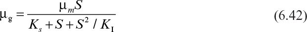
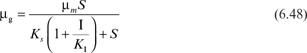
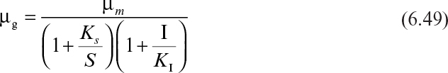
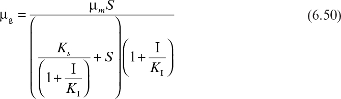
For noncompetitive substrate inhibition,
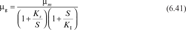
Or, if KI ≫ KS, then
For competitive substrate inhibition,
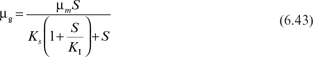
Note that equation 6.43 is different from equations 6.41 and 6.42, and KI in equations 6.42 and 6.43 is different. Substrate inhibition may be alleviated by slow, intermittent addition of the substrate to the growth medium.
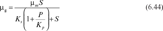
High concentrations of product can be inhibitory for microbial growth. Product inhibition may be competitive or noncompetitive, and in some cases when the underlying mechanism is not known, the inhibited growth rate is approximated to exponential or linear decay expressions.
Equations 6.44 and 6.45 present important examples of the product inhibition rate expression.
For competitive product inhibition,
For noncompetitive product inhibition,
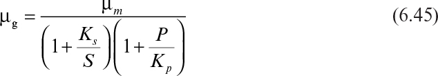
Ethanol fermentation from glucose by yeasts is a good example of noncompetitive product inhibition, and ethanol is the inhibitor at concentrations above about 5%. Other rate expressions used for ethanol inhibition are as follows:
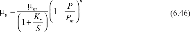
where Pm is the product concentration at which growth stops.

where Kp is the product inhibition constant.
Analogous to enzyme inhibition, the following rate expressions are used for competitive (eq. 6.48), noncompetitive (eq. 6.49), and uncompetitive (eq. 6.50) inhibition by an inhibitor other than substrate or product:
In some cases, the presence of toxic compounds in the medium results in the inactivation of cells or death. The net specific rate expression in the presence of death has the form
where k′d is the death-rate constant (h–1).
6.2.1.3. The logistic equation.
When plotted on arithmetic paper, the batch growth curve assumes a sigmoidal shape (see Figure 6.3). This shape can be predicted by combining the Monod equation (6.32) with the growth equation (6.2) and an equation for the yield of cell mass based on substrate consumption. Combining equations 6.32 and 6.2a and assuming no endogenous metabolism yields the following:
The relationship between microbial growth yield and substrate consumption is
where X0 and S0 are initial values, and YX/S is the cell mass yield based on the limiting nutrient. Substituting for S in equation 6.53 yields the following rate expression:

The integrated form of the rate expression in this phase is

This equation describes the sigmoidal-shaped batch growth curve, and the value of X asymptotically reaches to the value of YX/S S0 + X0.
Equation 6.54 requires a predetermined knowledge of the maximum cell mass in a particular environment. We denote this maximum cell mass as X∞; it is identical to the ecological concept of carrying capacity. Equation 6.55 is implicit in its dependence on S.
Logistic equations are a set of equations that characterize growth in terms of carrying capacity. The usual approach is based on a formulation in which the specific growth rate is related to the amount of unused carrying capacity:

Thus, we have the following:
The integration of equation 6.57 with the boundary condition X (0) = X0 yields the logistic curve:
Equation 6.58 is represented by the growth curve in Figure 6.12.
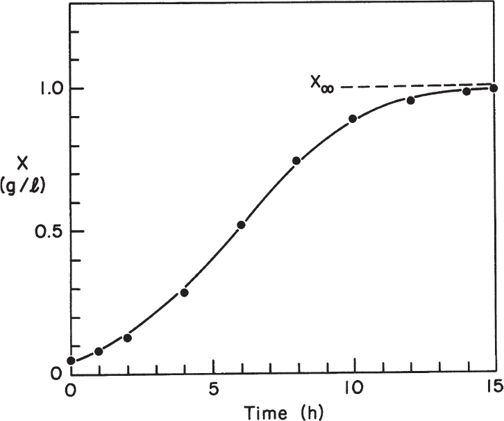
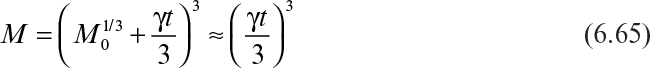
Equations of the form of 6.58 can also be generated by assuming that a toxin generated as a by-product limits the growth at X∞ (which is the carrying capacity allowed due to build-up of a toxin). Example 6.2 illustrates the use of the logistic approach.
a. By fitting the biomass data to the logistic equation, determine the carrying-capacity coefficient k.
b. Determine yield coefficients YP/S and YX/S.
a. Equation 6.57 can be rewritten as follows:
or

Here ![]() is average biomass concentration during Δt, and X∞ is about 10.8 g/l, since growth is almost complete at 30 hours. Thus we get the following data:
is average biomass concentration during Δt, and X∞ is about 10.8 g/l, since growth is almost complete at 30 hours. Thus we get the following data:

A value of k = 0.24h–1 would describe most of the data, although it would slightly underestimate the initial growth rate. Another approach would be to take the log of the preceding equation:

We then fit the data to this equation and estimate k from the intercept. In this case, k would be about 0.25 h–1.
b. The yields are estimated directly from the data as follows:

The estimate of YX/S is only approximate, as maintenance effects and endogenous metabolism have been neglected.
6.2.1.4. The Gompertz equation for batch growth and product formation.
Neither the logistic (equation 6.58) nor the integrated Monod (equation 6.55) equations consider the lag phase in batch microbial growth and product formation. The Gompertz equation considers the maximum growth potential, maximum growth rate, and duration of the lag phase in batch microbial growth and was developed originally to model the growth of tumors.
The Gompertz equation for batch microbial growth has the following form:
where X is the concentration of biomass at any time during batch growth, Xm is the maximum biomass concentration, Rxm is the maximum rate of growth, λ is duration of the lag phase, e is 2.718, and t is time.
A similar equation can be written for product formation:
where P is the concentration of product at any time during batch growth, Pm is the maximum potential product concentration, Rpm is the maximum rate of product formation, λ is duration of the lag phase, e is approximately 2.718, and t is time. It is assumed that initial biomass (Xo) and product (Po) concentrations are negligible in equations 6.59 and 6.60.
Variation of substrate concentration with time can be estimated by using the following equation:

With a negligible Xo, equation 6.61 takes the following form:

Due to inclusion of the lag time, Gompertz equations may correlate with the batch experimental data better than the logistic and the integrated Monod equations do.
6.2.1.5. Growth models for filamentous organisms.
Filamentous organ-isms such as molds often form microbial pellets at high cell densities in suspension culture. Cells growing inside pellets may be subject to diffusion limitations. The growth models of molds should include the simultaneous diffusion and consumption of nutrients within the pellet at large pellet sizes. This problem is the same one we face in modeling the behavior of bacteria or yeasts entrapped in spherical gel particles (see Chapter 9, “Operating Considerations for Bioreactors for Suspension and Immobilized Cultures”).
Alternatively, filamentous cells can grow on the surface of a moist solid. Such growth is usually a complicated process, involving not only growth kinetics but the diffusion of nutrients and toxic metabolic by-products. However, for an isolated colony growing on a rich medium, we can ignore some of these complications.
In the absence of mass-transfer limitations, it has been observed that the radius of a microbial pellet in a submerged culture or of a mold colony growing on an agar surface increases linearly with time:

In terms of growth rate of a mold colony, equation 6.63 can be expressed as

or

where γ = kP (36πρ)1/3. Integration of Equation 6.64b yields the following:
The initial biomass, M0, is usually very small compared to M, and therefore M varies with t3. This behavior has been supported by experimental data.
6.2.2. Models for Transient Behavior
In most practical applications of microbial cultures, the environmental or culture conditions can shift, dramatically leading to changes in cellular composition and biosynthetic capabilities. These cellular changes are not instantaneous but occur over an observable period of time. In this section, we examine models that can describe or predict such time-dependent (or transient) changes.
6.2.2.1. Models with time delays.
The unstructured growth models we have described so far are limited to balanced or pseudobalanced growth conditions. These unstructured models can be improved for use in dynamic situations through the addition of time delays. The use of time delays incorporates structure implicitly. It is built on the premise that the dynamic response of a cell is dominated by an internal process with a time delay on the order of the response time under observation. Other internal processes are assumed to be too fast (essentially always at a pseudoequilibrium) or too slow to influence greatly the observed response. By using black-box techniques equivalent to the traditional approach to the control of chemical processes, it is possible to generate transfer functions that can represent the dynamic response of a culture. An example of the results from such an approach is given in Figure 6.13. However, it should be recognized that such approaches are limited to cultures with similar growth histories and subjected to qualitatively similar perturbations.

Figure 6.13. Comparison of predictions from a model derived from a system-analysis perspective, predictions from a Monod model, and experiment. The experimental system was a chemostat for a glucose-limited culture of Saccharomyces cerevisiae operating at a dilution rate of 0.20 h–1. In this particular experiment, the system was perturbed with a stepwise increase in feed glucose concentration from 1.0 and 2.0 g l–1. X is biomass concentration, μ is growth rate, and S is substrate concentration. (With permission, from T. B. Young III and H. R. Bungay, “Dynamic Analysis of a Microbial Process: A Systems Engineering Approach,” Biotechnol. Bioeng. 15:377, 1973, and John Wiley & Sons, Inc., New York.)
6.2.2.2. Chemically structured models.
A much more general approach with much greater a priori predictive power is a model capturing the important kinetic interactions among cellular subcomponents. Initially, chemically structured models were based on two components, but at least three components appear necessary to give good results. More sophisticated models with 20 to 40 components are being used in many laboratories. A schematic of one such model is given in Figure 6.14.
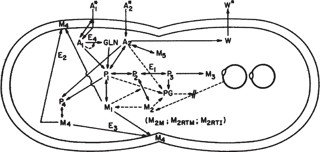
Figure 6.14. An idealized sketch of the model Escherichia coli B/rA growing in a glucose–ammonium salts medium with glucose or ammonia as the limiting nutrient. At the time shown, the cell has just completed a round of DNA replication and initiated cross-wall formation and a new round of DNA replication. Solid lines indicate the flow of material, and dashed lines indicate flow of information. The symbols are A1, ammonium ion; A2, glucose (and associated compounds in the cell); W, waste products (CO2, H2O, and acetate) formed from energy metabolism during aerobic growth; P1, amino acids; P2, ribonucleotides; P3, deoxyribonucleotides; P4, cell envelope precursors; M1, protein (both cytoplasmic and envelope); M2RTI, immature “stable” RNA; M2RTM, mature “stable” RNA (rRNA and tRNA—assume 85% rRNA throughout); M2M, messenger RNA; M3, DNA; M4, nonprotein part of cell envelope (assume 16.7% peptidoglycan, 47.6% lipid, and 35.7% polysaccharide); M5, glycogen; PG, ppGpp; E1, enzymes in the conversion of P2 to P3; E2, E3, molecules involved in directing cross-wall formation and cell envelope synthesis; GLN, glutamine; E4, glutamine synthetase; * indicates that the material is present in the external environment. (With permission, from M. L. Shuler and M. M. Domach, in Foundations of Biochemical Engineering, H. W. Blanch, E. T. Papoutsakis, and G. Stephanopoulos, ed., ACS Symposium Series 207, American Chemical Society, Washington, DC, 1983, p. 93.)
Writing such models requires that the modeler understand the physical system at a level of greater detail than that at which the model is written, so that the appropriate assumptions can be made. A detailed discussion of such models is appropriate for more advanced texts. However, two important guidelines in writing such models should be understood by even the beginning student. The first is that all reactions should be expressed in terms of intrinsic concentrations. An intrinsic concentration is the amount of a compound per unit cell mass or cell volume. Extrinsic concentrations, the amount of a compound per unit reactor volume, cannot be used in kinetic expressions. Although this may seem self-evident, all the early structured models were flawed by the use of extrinsic concentrations. A second consideration, closely related to the first, is that the dilution of intrinsic concentration by growth must be considered.
The appropriate equation to use in a nonflow reactor is

where VR is the total volume in the reactor, X is the extrinsic biomass concentration, and Ci is the extrinsic concentration of component i.
Equation 6.66 can also be rewritten in terms of intrinsic concentrations. For simplicity, we use mass fractions (e.g., Ci/X). Note the following:

Recall equation 6.2a:
We now have

Substituting equation 6.66 for (1/X)(dCi/dt) after dividing the equation by VRX and assuming VR is a constant, we get the following:

In equation 6.69, the rfi term must be in terms of intrinsic concentrations and the term μnetCi/X represents dilution by growth. These concepts are illustrated in Example 6.3.
The model indicated in Figure 6.14 is that for a single cell. The single-cell model response can be directly related to culture response if all cells are assumed to behave identically. In this case, each cell has the same division cycle. A population will have, at steady state, twice as many cells at “birth” as at division. The average concentrations in the culture will be at the geometric mean (a time equal to ![]() multiplied by the division time) for each cell component. Used in this way, the model is a structured, nonsegregated model. If, however, a cellular population is divided into subpopulations, with each subpopulation represented by a separate single-cell model, then a population model containing a high level of structure, as well as aspects of segregation, can be built.
multiplied by the division time) for each cell component. Used in this way, the model is a structured, nonsegregated model. If, however, a cellular population is divided into subpopulations, with each subpopulation represented by a separate single-cell model, then a population model containing a high level of structure, as well as aspects of segregation, can be built.
Such a finite-representation technique has been used and is capable of making good a priori predictions of dynamic response in cultures (see Figure 6.15). When used in this context, at least one random element in the cell cycle must be included to lead to realistic prediction of distributions. Some examples of such randomness include placement of the cell cross wall, timing of the initiation of chromosome synthesis or cross-wall synthesis, and distribution of plasmids at division. Models that incorporate genomic detail have been developed. Such models reveal the explicit relationship of genetic modifications to physiological response. While these models are beyond the scope of an introductory text, be aware that many advances have been made in this regard.
Figure 6.15. Prediction of transient response in a continuous-flow system to perturbations in limiting substrate concentration or flow rate. Note that the predictions are not fitted to the data; predictions are completely a priori. (a) Transient glucose concentration in response to step change in glucose feed concentration from 1.0 to 1.88 g/l in anaerobic continuous culture of Escherichia coli B/r at dilution rate of 0.38 h–1; ![]() and
and ![]() , results of two duplicate experimental runs; solid line, computer prediction. (b) Transient glucose concentration in response to step change in dilution rate from D = 0.16 to D = 0.55 h–1;
, results of two duplicate experimental runs; solid line, computer prediction. (b) Transient glucose concentration in response to step change in dilution rate from D = 0.16 to D = 0.55 h–1; ![]() and
and ![]() , results of two duplicate experimental runs; solid line, computer prediction. (With permission, from M. M. Ataai and M. L. Shuler, Simulation of CFSTR through development of a mathematical model for anaerobic growth of Escherichia coli cell population. Biotechnol. Bioeng. 27:7, p. 1051, 1985, and John Wiley & Sons, Inc., New York.)
, results of two duplicate experimental runs; solid line, computer prediction. (With permission, from M. M. Ataai and M. L. Shuler, Simulation of CFSTR through development of a mathematical model for anaerobic growth of Escherichia coli cell population. Biotechnol. Bioeng. 27:7, p. 1051, 1985, and John Wiley & Sons, Inc., New York.)
With this section, you should have a good overview of the basic concepts in modeling and some simple tools to describe microbial growth. We need these tools to adequately discuss the cultivation of cells in continuous culture. Example 6.3 illustrates how a structured model might be developed.


6.2.3. Cybernetic Models
Another modeling approach has been developed primarily to predict growth under conditions when several substrates are available. These substrates may be complementary (e.g., carbon or nitrogen) or substitutable. For example, glucose and lactose would be substitutable, as these compounds both supply carbon and energy. We discussed the diauxic phenomenon for sequential use of glucose and lactose in Chapter 4, “How Cells Work.” That experimental observation led us to an understanding of regulation of the lac operon and catabolite repression. This metabolic regulation was necessary for the transition from one primary pathway to another. We might infer that the culture had as its objective function the maximization of its growth rate.
One approach to modeling growth on multiple substrates is a cybernetic approach. Cybernetic means that a process is goal seeking (e.g., maximization of growth rate). While this approach was initially motivated by a desire to predict the response of a microbial culture to growth on a set of substitutable carbon sources, it has been expanded to provide an alternative method of identifying the regulatory structure of a complex biochemical reaction network (such as cellular metabolism) in a simple manner. Typically, a single objective, such as maximum growth rate, is chosen and an objective-oriented mathematical analysis is employed. This analysis is similar to many economic analyses for resource distribution. For many practical situations, this approach describes satisfactorily growth of a culture on a complex medium. However, the potential power of this approach is now being realized in metabolic engineering and in relating information on DNA sequences to physiological functions of organisms (see Chapter 8, “How Cellular Information Is Altered”).
This approach has limitations, as the objective function for any organism is maximizing its long-term survival as a species. Maximization of growth rate or of growth yield are really subobjectives that can dominate under some environmental conditions; these conditions are often of great interest to the bioprocess engineer. Consequently, the cybernetic approach is often a valuable tool. It is too complex for us to describe in detail in this book; consult the references at the end of this chapter for more information.
6.3. Cell Growth In Continuous Culture
The culture environment changes continually in a batch culture. Growth, product formation, and substrate utilization terminate after a certain time interval, whereas in continuous culture, fresh nutrient medium is continually supplied to a well-stirred culture, and products and cells are simultaneously withdrawn. Growth and product formation can be maintained for prolonged periods in continuous culture. After a certain period of time, the system usually reaches a steady state where cell, product, and substrate concentrations remain constant. Continuous culture provides constant environmental conditions for growth and product formation and supplies uniform-quality product. Continuous culture is an important tool to determine the response of microorganisms to their environment and to produce the desired products under optimal environmental conditions. In Chapter 9, we will compare batch and continuous culture in terms of their suitability for large-scale operation.
6.3.1. Specific Devices for Continuous Culture
The primary types of continuous cultivation devices are the chemostat and turbidostat, although plug flow reactors (PFRs) are used. In some cases, these units are modified by the recycling of cells.
Figure 6.16 is a schematic of a continuous culture device (chemostat). Cellular growth is usually limited by one essential nutrient, and other nutrients are in excess. As we will show, when a chemostat is at steady state, the nutrient, product, and cell concentrations are constant. For this reason, the name chemostat refers to constant chemical environment.

Figure 6.16. A continuous-culture laboratory setup (chemostat). (With permission, from D. I. C. Wang and others, Fermentation and Enzyme Technology, John Wiley & Sons, Inc., New York, 1979, p. 99. Permission conveyed through Copyright Clearance Center, Inc.)
Figure 6.17 is a schematic of a turbidostat in which the cell concentration in the culture vessel is maintained constant by monitoring the optical density of the culture and controlling the feed flow rate. When the turbidity of the medium exceeds the set point, a pump is activated and fresh medium is added. The culture volume is kept constant by removing an equal amount of culture fluid. The turbidostat is less used than the chemostat, since it is more elaborate than a chemostat and because the environment is dynamic. Turbidostats can be very useful in selecting subpopulations able to withstand a desired environmental stress (e.g., high ethanol concentrations), because the cell concentration is maintained constant. The selection of variants or mutants with desirable properties is very important (see Chapter 8).
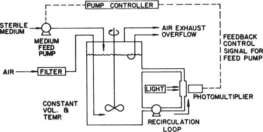
Figure 6.17. Typical laboratory setup for a turbidostat. (With permission, from D. I. C. Wang and others, Fermentation and Enzyme Technology, John Wiley & Sons, Inc., New York, 1979, p. 100. Permission conveyed through Copyright Clearance Center, Inc.)
A PFR can also be used for continuous cultivation purposes. Since there is no backmixing in an ideal PFR, fluid elements containing active cells cannot inoculate other fluid elements at different axial positions. Liquid recycle is required for continuous inoculation of nutrient media. In a PFR, substrate and cell concentrations vary with axial position in the vessel. An ideal PFR resembles a batch reactor in which distance along the fermenter replaces incubation time in a batch reactor. In waste treatment, some units approach PFR behavior, and multistage chemostats tend to approach PFR dynamics if the number of stages is large (five or more).
6.3.2. The Ideal Chemostat
An ideal chemostat is the same as a perfectly mixed continuous-flow, stirred-tank reactor (CFSTR). Most chemostats require some control elements, such as pH and DO control units, to be useful. Fresh sterile medium is fed to the completely mixed and aerated (if required) reactor, and cell suspension is removed at the same rate. Liquid volume in the reactor is kept constant. A critical feature of a chemostat is that a steady state arises spontaneously where the growth rate is determined by the feed flow rate to per unit of reactor volume (or dilution rate as defined in equation 6.71).
Figure 6.18 is a schematic of a simplified chemostat. A material balance on the cell concentration around the chemostat yields


where F is the flow rate of nutrient solution (l/h), VR is the culture volume (l) (assumed constant), X is the cell concentration (g/l), and μg and kd are growth and endogenous (or death) rate constants, respectively (h–1). Note that if cell mass is the primary parameter, it is difficult to differentiate cell death from endogenous metabolism. When we use kd, we imply that endogenous metabolism is the primary mechanism for cell mass decrease. With k′d, we imply that cell death and lysis are the primary mechanisms of decrease in mass. Also note that if equation 6.70 had been written in terms of cell number, kd could only be a cell death rate. When balances are written in terms of cell number, the influence of endogenous metabolism can appear only in the substrate balance equation. Since most experiments are done by measuring total cell mass rather than number, we write our examples based on X. However, be aware of the ambiguity introduced when equations are written in terms of X.
Equation 6.70 can be rearranged as follows:

where D is dilution rate and D = F/VR. D is the reciprocal of hydraulic residence time (V/F).
Usually, the feed media are sterile, X0 = 0, and if the endogenous metabolism or death rate is negligible compared to the growth rate (kd ≪ μg) and if the system is at steady state (dX/dt = 0), then we get the following:
In a chemostat, cells are removed at a rate equal to their growth rate, and the growth rate of cells is equal to the dilution rate. This property allows the investigator to manipulate growth rate as an independent parameter and makes the chemostat a powerful experimental tool.
Since growth rate is limited by at least one substrate in a chemostat, a simple description of chemostat performance can be made by substituting the Monod equation (equation 6.32) for μg in equation 6.72:

Here S is the steady-state limiting substrate concentration (g/l). If D is set at a value greater than μm, the culture cannot reproduce quickly enough to maintain itself and is washed out (i.e., no substrate is used [S = S0] and no biomass is formed [X = 0]). Equation 6.73 is identical to that for Michaelis–Menten kinetics, and as we discussed in Chapter 3, “Enzymes,” a plot of 1/μg versus 1/S can be used to estimate values for μm and Ks.
Using equation 6.73, we can relate effluent substrate concentration to dilution rate for D < μm:
A material balance on the limiting substrate yields the following:
Here S0 and S are feed and effluent substrate concentrations (g/l), qP is the specific rate of extracellular product formation (g P/g X-h), YMX/S, and YP/S are yield coefficients (g X/g S and gP/gS), and ms is the maintenance coefficient based on substrate (g S/g X-h). The use of the superscript M on YX/S denotes a maximum value of the yield coefficient; such a superscript will be important in discussing the effects of maintenance energy. Equation 6.75 can be written as follows:

Equation 6.76 is known as the linear equation of substrate consumption, which is an explicit expression of the substrate balance given by equation 6.14.
When the extracellular product formation and the maintenance are negligible (qp and ms are negligible) and the system is at steady state (dS/dt = 0), equation 6.76 takes the following form:
Since μg = D at steady state, if kd = 0, then we have the following:
Using equation 6.74, the steady-state cell concentration can be expressed as follows:
In equations 6.77 and 6.78, the yield coefficient (YX/S) is assumed to be constant and equal to ![]() , which is an approximation, since endogenous metabolism has been neglected. Usually, YX/S varies with the limiting nutrient and growth rate. When endogenous metabolism or death rate are not negligible, equation 6.72 takes the following form:
, which is an approximation, since endogenous metabolism has been neglected. Usually, YX/S varies with the limiting nutrient and growth rate. When endogenous metabolism or death rate are not negligible, equation 6.72 takes the following form:
or
By substituting Equation 6.80b into the steady-state substrate balance, assuming no extracellular product formation (equation 6.77), we find the following:
Here ![]() denotes the maximum yield coefficient (no endogenous metabolism or maintenance energy).
denotes the maximum yield coefficient (no endogenous metabolism or maintenance energy). ![]() is constant and independent of growth rate. Since this approach is based on an unstructured model, it does not allow the direct conversion of extracellular substrates into maintenance energy. Rather, S must be first incorporated into the cell mass, where it is degraded by endogenous metabolism. This viewpoint is the proper one when working with an unstructured model. With a structured model, which explicitly recognizes intracellular S as a subcomponent of the biomass, the direct consumption of S for maintenance functions could be modeled. However, with unstructured models, substrate that is no longer extracellular becomes part of the biomass, X.
is constant and independent of growth rate. Since this approach is based on an unstructured model, it does not allow the direct conversion of extracellular substrates into maintenance energy. Rather, S must be first incorporated into the cell mass, where it is degraded by endogenous metabolism. This viewpoint is the proper one when working with an unstructured model. With a structured model, which explicitly recognizes intracellular S as a subcomponent of the biomass, the direct consumption of S for maintenance functions could be modeled. However, with unstructured models, substrate that is no longer extracellular becomes part of the biomass, X.
Equation 6.80c can be rearranged as follows:

or
or

where

where ms is the maintenance coefficient based on substrate S. ![]() is the apparent yield. When YX/S is written, it should be interpreted as
is the apparent yield. When YX/S is written, it should be interpreted as ![]() . While
. While ![]() is a constant,
is a constant, ![]() varies with growth conditions if kd > 0.
varies with growth conditions if kd > 0.
Values of ![]() and ms can be obtained from chemostat experiments by plotting 1/
and ms can be obtained from chemostat experiments by plotting 1/![]() against 1/D. The slope is ms and the intercept is 1/
against 1/D. The slope is ms and the intercept is 1/![]() (see Figure 6.19).
(see Figure 6.19).

Figure 6.19. Graphical approach to estimating ![]() and mS for chemostat data for Escherichia coli growing on glucose as the limiting nutrient.
and mS for chemostat data for Escherichia coli growing on glucose as the limiting nutrient.
In the presence of endogenous metabolism [μnet = μmS/(Ks + S) – kd], we can also show the following:


In addition to the effects of maintenance, it is often appropriate to consider the conversion of extracellular substrate into extracellular product. With an unstructured model, we must view this as instantaneous conversion. Otherwise, a perceptible period of substrate uptake, prior to conversion to product, would cause a change in the amount of X. This is unlike maintenance, since the period between substrate uptake and use for maintenance functions may be long, so we allow S to become incorporated into X, and X is then degraded when needed; the following equations assume instantaneous conversion of substrate to extracellular product, with the cell acting as a catalyst. The balance on product formation is
where qP is described by equation 6.19 or 6.20. For nongrowth-associated product formation, qP is constant (β), and for growth-associated products, it is a function of μg. In the presence of product formation and with negligible maintenance, equation 6.76 becomes

The biomass balance is unchanged from the case with endogenous metabolism (given in eq. 6.85) and yields
Equation 6.87 can be solved for X:
The productivity of a chemostat for product and biomass (Prx) can be found from DP and DX, respectively. The dilution rate that maximizes productivity is found by differentiating DP or DX with respect to D and setting the derivative equal to zero. The optimal value of D (Dopt) will depend on whether endogenous metabolism and/or product formation are considered. When kd = 0 and qP = 0, equations 6.78 and 6.74 apply. Then Dopt for biomass production (DX) becomes

Since S0 is usually much greater than Ks, Dopt will approach D = μm, or the washout point. Stable chemostat operation with D ⋍ μm is very difficult unless the flow rate and liquid volume can be maintained exactly constant. Consequently, a value of D slightly less than Dopt may be a good compromise between stability and biomass productivity. It should also be apparent that Dopt for biomass formation will not necessarily be optimal for product formation.
Examples 6.4 and 6.5 illustrate the use of these equations to characterize the performance of chemostats.
Example 6.4. Calculating Basic Chemostat Parameters
A new strain of yeast is being considered for biomass production. The following data were obtained using a chemostat. An influent substrate concentration of 800 mg/l and an excess of oxygen were used at a pH of 5.5 and T = 35°C. Using the following data, calculate μm, Ks, ![]() , kd, and ms, assuming μnet = μmS/(Ks + S) – kd.
, kd, and ms, assuming μnet = μmS/(Ks + S) – kd.
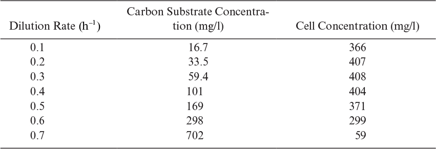
Solution The first step is to plot ![]() versus
versus ![]() . is calculated from X/(S0 – S). The intercept is
. is calculated from X/(S0 – S). The intercept is ![]() or
or ![]() . The slope is 0.06 g S/g X-h, which is the value for ms. Recall
. The slope is 0.06 g S/g X-h, which is the value for ms. Recall ![]() ; then
; then ![]() . For the second step, recall the following:
. For the second step, recall the following:


Example 6.5. Effect of Inhibitors on Chemostat Growth

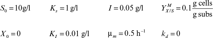
a. Determine X and S as a function of D when I = 0
b. With inhibitor added to a chemostat, determine the effluent substrate concentration and X as a function of D.
c. Determine the cell productivity, DX, as a function of dilution rate.
a. The following equations apply when there is no inhibitor:
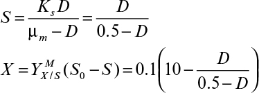
b. In the presence of inhibitor, we use the following:
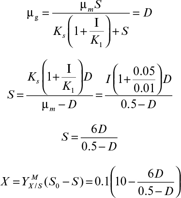
c. The cell productivity can then be calculated from the following:
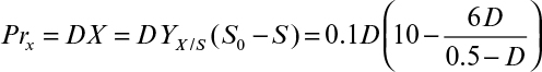
6.3.3. The Chemostat as a Tool
The chemostat can be used as a tool to study the mutation and selection of cultures and also to study the effect of changes in the environment on cell physiology. The molecular aspects of mutation and selection are discussed in Chapter 8.
Natural or induced mutations can take place in a chemostat culture. Errors in DNA replication take place with an average frequency of about 10–6 to 10–8 genes per generation. With a cell concentration of 109 cell/ml in culture, the probability is high in a chemostat that a wide variety of mutant cells will be formed. The vast majority of natural mutations in a chemostat are of little significance unless the mutation alters the function of a protein involved in growth in the chemostat environment. If the specific growth rate of the mutant is larger than that of the wild type, then the mutant outgrows the wild type in a chemostat. This selection for a variant cell type can be accomplished by creating a more favorable environment for growth of the mutant organism.
A chemostat culture can be used for the selection of special organisms. Selection or enrichment nutrient media need to be used for this purpose. For example, if it is desired to select an organism growing on ethanol, a nutrient medium containing ethanol and mineral salts is used as a feed to a chemostat culture. An organism capable of oxidizing some toxic refractory compounds can be selected from a mixed culture by slowly feeding this compound to a chemostat. A thermophilic organism can be selected from a natural population by operating a chemostat at an elevated temperature (e.g., 50° to 60°C). Selection in chemostats also presents significant problems in the culture of cells containing recombinant DNA. The most productive cells often grow more slowly and are displaced by less productive cells. We discuss this problem in more detail in Chapter 14, “Utilizing Genetically Engineered Organisms.”
6.3.4. Deviations from Ideality
In fermentations such as the utilization or production of polysaccharides or mycelial fermentations, the fermentation broth may be highly viscous and it may be difficult to maintain complete mixing. Also, certain cells tend to grow in the form of a film on solid surfaces in fermenters, such as on fermenter walls or probe surfaces. Incomplete mixing is the rule in industrial-scale fermenters. The presence of incompletely mixed regions in a “chemostat” culture is common. The term chemostat is actually applicable only to perfectly mixed vessels. Here we denote nonideality by putting “chemostat” in quotation marks. A segregated reactor model can be used to analyze an incompletely mixed continuous-flow fermenter.
A simple, two-compartmental model of a “chemostat” culture is depicted in Figure 6.20, where the reactor is divided into two regions: a well-mixed region and a stagnant region. Feed and effluent streams pass through the well-mixed region 1, and mass exchange takes place between the two regions.
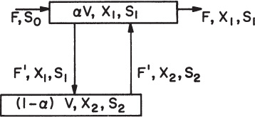
In an imperfectly mixed chemostat with a stagnant biotic phase, the dilution rate can exceed μm without washout. The washout dilution rate is obtained by setting S0 = S1 = S2:
where Dwo is the washout dilution rate.
6.4. Summary
During batch cultivation, a population of cells typically exhibits several different growth phases. During the lag phase, the cell builds the biosynthetic pathways necessary for maximal growth rates in the fresh medium. During exponential growth, cell replication is maximal, and the chemical composition of the cell population is nearly constant (e.g., balanced growth). When substrate is nearly exhausted or when toxic metabolic by-products have built to a critical level, the growth rate begins to drop rapidly, causing significant changes in biosynthetic pathways. In the stationary phase, there is no net growth; cells now reorient their metabolic machinery to increase the probability of long-term survival. At some point, some cells can no longer obtain enough energy from their reserves or enough of another critical resource, and the culture enters the death phase. Dead cells do not have an energized membrane and often lyse (or break apart). Nutrients released by lysed cells can be utilized by survivors, allowing cryptic growth.
Products formed by cells can be related to this batch-culture growth cycle. Primary products are growth associated. Secondary products are nongrowth associated and are made in the stationary phase. Some products have both growth-associated and nongrowth-associated components.
Cell-growth kinetics can be modeled. Models that are structured break the population into distinct subcomponents. Unstructured models quantify cell mass as a single component. Unstructured models cannot describe transient behavior very well. Some models are segregated; they recognize that not all members of the population are identical, and the distribution of properties among individual cells is important. Nonsegregated models ignore these distributions and assume that population-average parameters are adequate.
These models apply not only to batch culture but also to continuous culture. The primary form of continuous culture is a steady-state CFSTR, or chemostat. A chemostat ensures a time-invariant growth environment. The net growth rate is equal to the dilution rate, which is determined by the flow rate to the chemostat. Thus, the growth rate can be manipulated by the investigator. A turbidostat adjusts flow rate to maintain a constant cell density. A turbidostat operates well at high flow rates (near the washout point) and is useful in selecting cellular subpopulations that have adapted to a particular stress.
Suggestions for Further Reading
ATLAS, J. P., P. FOLEY, AND M. L. SHULER, “Modeling a Minimal Cell,” Meth. Mol. Biol. 881: 573–610, 2012.
BAILEY, J. E., AND D. F. OLLIS, Biochemical Engineering Fundamentals, 2d ed., McGraw-Hill, New York, 1986.
BLANCH, H. W., AND D. S. CLARK, Biochemical Engineering, Marcel Dekker, New York, 1996.
DORAN, P. M., Bioprocess Engineering Properties, 2d ed., Academic Press, San Diego, CA, 2013.
FREDERICKSON, A. G., R. D. MEGEE III, AND H. M. TSUCHIYA, “Mathematical Models for Fermentation Processes,” Adv. Appl. Microbiol. 23(10): 419, 1970.
RAMKRISHNA, D., AND H. SONG, “Dynamic Models of Metabolism: Review of the Cybernetic Approach,” AIChE Journal 58: 986–992, 2012.
VILLADSEN, J., J. NIELSEN, AND G. LIDEN, Bioreaction Engineering Principles, 2d ed., Springer, New York, 2011.
Problems
6.1. By using the following information, determine the cell number concentration in a fermenter containing 1 g dry weight/l biomass:
Cell dimensions: 1 × 2 μm cylindrical cells
Cell density: 1.05 g/cm3
Water content of cells: 80%
6.2. Two different bacterial species with doubling times of 2 h and 4 h are growing in a batch nutrient-rich medium with their maximum growth rate. The initial concentrations are the same.
a. What would be the ratio of X1/X2 after 10 h of batch growth?
b. How long should the batch growth of the mixed cultures last in order to obtain X1/X2 = 10? Assume exponential growth.
6.3. A simple, batch fermentation of an aerobic bacterium growing on methanol gave the results shown in the following table. Calculate the following:
a. Maximum growth rate (μmax)
b. Yield on substrate (YX/S)
c. Mass doubling time (td)
d. Saturation constant (Ks)
e. Specific growth rate (μnet) at t = 10 h
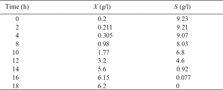
6.4. The growth of a microbial population is a function of pH and is given by the following equation:
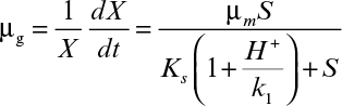
a. With a given set of experimental data (X and S versus t), describe how you would determine the constants μm, Ks, and k1.
b. How would the double-reciprocal plot 1/μg versus 1/S change with pH (or H+) concentration?
6.5. The following data were obtained for the effect of temperature on the fermentative production of lactic acid by a strain of Lactobacillus delbrueckii. From these data, calculate the value of the activation energy for this process. Is the value of the activation energy typical of this sort of biological conversion? (See Chapter 3.)
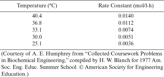
6.6. The logistic equation for batch microbial growth is given by the following equation:

a. Use the following approximations:
Xm = Yx/s S0, X =Yx/s (S0 -S)
Prove that the logistic equation can be expressed as follows:

b. By using the following relationship, develop an expression describing the variation of substrate concentration with time according to the logistic equation:
c. By comparing the form of logistic equation derived in part (a) with the Monod equation at low substrate concentrations (first-order kinetics), determine the logistic equation constant (k) in terms of Monod kinetic constants.
6.7. It is desired to model the growth of an individual bacterium. The cell transports S1 into the cell enzymatically, and the permease is subject to product inhibition. S1 is converted into precursors, P, that are converted finally into the macromolecular portion of the cell, M. The catalyst of all reactions is M.
a. ![]() (per unit surface area), where S* = outside concentration of S
(per unit surface area), where S* = outside concentration of S
b. ![]()

c2. Or, ![]()
d. The dry weight of the cell is T and is equal to T = S1 + P + M1 = ρV, where ρ = cell density and V = cell volume
Write the mass balance equations and define all symbols necessary to describe the changes in S1, P, M, and T within the cell. Remember that the cell volume is always changing.
6.8. A biochemical engineer has determined in her lab that the optimal productivity of a valuable antibiotic is achieved when the carbon nutrient, in this case molasses, is metered into the fermenter at a rate proportional to the growth rate. However, she cannot implement her discovery in the antibiotic plant, since there is no reliable way to measure the growth rate (dx / dt) or biomass concentration (X) during the course of the fermentation. It is suggested that an oxygen analyzer be installed on the plant fermenters so that the OUR (oxygen uptake rate, g/l-h) may be measured.
a. Derive expressions that may be used to estimate X and dX / dt from OUR and time data, assuming that a simple yield and maintenance model may be used to describe the rate of oxygen consumption by the culture.
b. Calculate values for the yield (YX/O2) and maintenance (mO2) parameters from the following data:
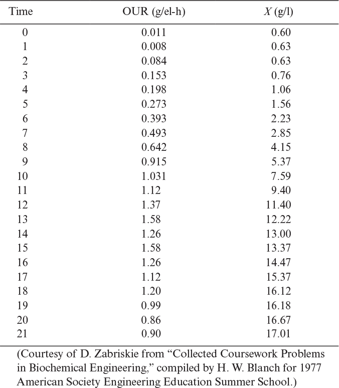
6.9. Pseudomonas sp. has a mass doubling time of 2.4 h when grown on acetate. The saturation constant using this substrate is 1.3 g/l (which is unusually high), and cell yield on acetate is 0.46 g cell/g acetate. If we operate a chemostat on a feed stream containing 38 g/l acetate, find the following:
a. Cell concentration when the dilution rate is one-half of the maximum
b. Substrate concentration when the dilution rate is 0.8 Dmax
c. Maximum dilution rate
d. Cell productivity at 0.8 Dmax
(Courtesy of E. Dunlop from “Collected Coursework Problems in Biochemical Engineering,” compiled by H. W. Blanch for 1977 Am. Soc. Eng. Educ. Summer School. © American Society for Engineering Education.)
6.10. The following data were obtained in a chemostat for the growth of E. aerogenes on a glycerol-limited growth medium:
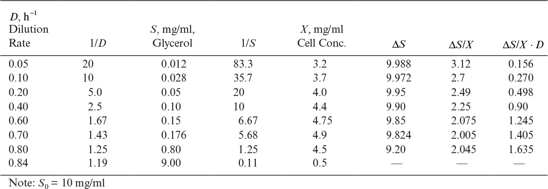
For this system, estimate the following values:
a. Ks, mg glycerol/ml
b. μm, h-1
c. YX/S, mg cells/mg glycerol
d. ms, mg glycerol/mg cell-h
(Courtesy of A. E. Humphrey from “Collected Coursework Problems in Biochemical Engineering,” compiled by H. W. Blanch for 1977 American Society for Engineering Summer School. © American Society for Engineering Education.)
6.11. The kinetics of microbial growth, substrate consumption, and mixed-growth-associated product formation for a chemostat culture are given by the following equations:

The kinetic parameter values are μm = 0.7 h–1, Ks = 20 mg/l, YX/S = 0.5 g dw/g substrate, YP/X = 0.15 gP/g·dw, α = 0.1, and S0 = 1 g/l.
a. Determine the optimal dilution rate maximizing the productivity of product formation (PD) when β = 0.02 h-1 and 0.01 h-1.
b. Determine the optimal dilution rate maximizing the productivity of cell (biomass) formation for the same value of β as in part (a) (DX).
(Problem adapted from one suggested by L. Erickson and modified by C. Lee.)
6.12. Ethanol is to be used as a substrate for single-cell protein production in a chemostat. The available equipment can achieve an oxygen transfer rate of 10 g O2/l of liquid per hour. Assume the kinetics of cell growth on ethanol is of the Monod type, with μm = 0.5 h–1, Ks = 30 mg/l, YX/S = 0.5 cells/g ethanol, and YO2/S = 2 g O2/g EtOH. We wish to operate the chemostat with an ethanol concentration in the feed of 22 g/l. We also wish to maximize the biomass productivity and minimize the loss of unused ethanol in the effluent. Determine the required dilution rate and whether sufficient oxygen can be provided.
6.13. Plot the response of a culture to diauxic growth on glucose and lactose based on the following: μglucose = 1.0 h–1, μlactose = 0.6 h–1, Yglucose = Ylactose = 0.5; enzyme induction requires 30 min to complete. Plot cell mass, glucose, and lactose concentrations, assuming initial values of 2 g/l glucose, 3 g/l lactose, and 0.10 g/l cells.
6.14. The following data are obtained in oxidation of pesticides present in wastewater by a mixed culture of microorganisms in a continuously operating aeration tank:

Assuming the pesticide concentration in the feed wastewater stream as S0 = 500 mg/l, determine ![]() , kd, μm, and Ks
, kd, μm, and Ks
6.15. Wastewater is treated in a completely mixed aeration tank operated in continuous mode. The rate of chemical oxygen demand (COD) removal is given by the following equation:
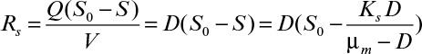
Here μm is the maximum specific growth rate constant (h–1), D is the dilution rate (h–1), Ks is saturation constant (mg/L), and S is the effluent COD concentration (mg/l).
a. Determine the optimum dilution rate or hydraulic residence time (HRT) maximizing COD removal rate.
b. Determine the optimal HRT, the maximum Rs and the biomass concentration for aerobic treatment where μm = 0.1 h–1, Ks = 0.1 g/l, Y = 0.4 gX/g S, and S0 = 1 g/l.
c. Determine the optimal HRT, the maximum Rs and biomass concentration for anaerobic treatment where μm = 0.01 h–1, Ks = 0.25 g/l, Y = 0.06 gX/g S, and S0 = 1 g/l.
6.16. Pseudomonas putida is used for fermentation of lactose present in cheese whey in a continuously operating aeration tank at a dilution rate of D = 0.28 h–1. The lactose concentration in the feed and the effluent are S0 = 2 g/L and Se = 0.1 g/l. The growth rate and lactose removal is limited by oxygen transfer. The following information is available: Yx/sM = 0.45 gX/g S, Yx/O2 = 0.25 gX/g O2 and C* = 8 mg/l (saturation DO).
a. Determine the steady-state biomass concentration (X) and the specific rate of oxygen consumption (qO2).
b. What should be the oxygen transfer coefficient (KLa) to overcome oxygen transfer limitations if the desired DO concentration in the fermentation medium is 2 mg/l?
6.17. In a chemostat, you know that if a culture obeys the Monod equation, the residual substrate is independent of the feed substrate concentration. You observe that in your chemostat, an increase in S0 causes an increase in the residual substrate concentration. Your friend suggests that you consider whether the Contois equation may describe the situation better. The Contois equation (equation 6.38) follows:
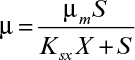
a. Derive an expression for S in terms of D, μm, Ksx, and X for a steady-state CFSTR (chemostat).
b. Derive an equation for S as a function of S0, D, Ksx, ![]() , and μm.
, and μm.
c. If S0 increases twofold, by how much will S increase?
6.18. The maximum growth yield coefficient for Bacillus subtilis growing on methanol is 0.4 g X/g S. The heat of combustion of cells is 21 kJ/g cells, and for substrate it is 7.3 kcal/g. Determine the metabolic heat generated by the cells per unit mass of methanol consumption.
6.19. Calculate the productivity (i.e., DP) of a chemostat under the following conditions:
a. Assume Monod kinetics applies. Assume that negligible amounts of biomass (<1%) must be converted to product.
b. Assume the Luedeking–Piret equation for product formation (equation 6.20) applies.
c. Assume steady state:
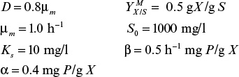
6.20. Consider a chemostat. You wish to know the number of cells in the reactor and the fraction of the cells that are viable (i.e., alive as determined by ability to divide).
a. Write an equation for viable cell number (nv). Assume the following:
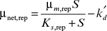
Here μnet,rep = net specific replication rate, μm,rep = maximum specific replication rate, and k′d = death rate. Ks,rep is the saturation parameter.
b. Derive an expression for the value of S at steady state.
c. Write the number balance in the chemostat on dead cells (nd).
d. Derive an expression for the fraction of the total population which are dead cells.
6.21. E. coli is cultivated in continuous culture under aerobic conditions with a glucose limitation. When the system is operated at D = 0.2 h–1, determine the effluent glucose and biomass concentrations by using the following equations (S0 = 5 g/l):
a. Monod equation: μm = 0.25 h–1, Ks = 100 mg/l
b. Tessier equation: μm = 0.25 h–1, K = 0.005 (mg/l)–1
c. Moser equation: μm = 0.25 h–1, Ks = 100 mg/l, n=1.5
d. Contois equation: μm = 0.25 h–1, Ksx = 0.04, ![]() = 0.4 g X/g S
= 0.4 g X/g S
S0 = 5 g/l
Compare and comment on the results.
6.22. Consider steady-state operation of a chemostat. Assume that growth is substrate inhibited and that endogenous metabolism can be ignored such that we get the following:

a. Derive an expression for the residual substrate concentration (i.e., S) as a function of dilution rate and the kinetic parameters (μm, KS, KI).
b. What are the implications for operation of a chemostat when the organism is subjected to substrate inhibition?
6.23. Formation of lactic acid from glucose is realized in a continuous culture by Streptococcus lactis. The following information was obtained from experimental studies:

a. Plot the variations of S, X, P, DX, and DP with dilution rate.
b. Determine (graphically) the optimum dilution rate maximizing the productivities of biomass (DX) and the product (DP).