
Chapter 5. The Physical Layer
You see, wire telegraph is a kind of a very, very long cat. You pull his tail in New York and his head is meowing in Los Angeles. Do you understand this? And radio operates exactly the same way: you send signals here, they receive them there. The only difference is that there is no cat.
—Albert Einstein
5.1. Background
Two or more Bluetooth low energy devices use radio waves to send and receive information among them. Radio has been around for many years, starting with very simple spark-gap transmitters, evolving through amplitude modulation and frequency modulation, and recently, to phase-shift keying and other more complex modulation schemes.
The sections that follow provide an introduction to how radios work, from the basics up to modern modulation schemes that are used by Bluetooth low energy.
5.2. Analog Modulation
The basic spark-gap radio is possibly the simplest radio that you can build. It is so simple that you could build it with just two components. Take a nine-volt battery with the two battery terminals at the top of the battery and a metal coin that can conduct electricity. But before you make your transmitter, you need to set up a receiver; you can use a radio that is turned to the AM band but not to any particular radio station. Then, briefly contact the coin to the battery terminals. You should hear the radio pick up the interference caused by the coin and the battery as the electricity sparks across the gap when the coin is very close to the terminals at the top of the battery but not actually touching them.
There are two problems with spark-gap radios. First, they are not very efficient. You need a very large electrical potential difference to transmit a long distance, typically many thousands of volts. Second, there is only one radio able to transmit at the same time in the same area. This severely restricts the ability to communicate more than one message at the same time in any given region. For example, imagine the residents of an entire city having the “choice” of just one television station.
The next advance in radio technology was amplitude modulation, or AM radio. It was observed that you could transmit a single frequency by using radio waves. These carrier signals could then be modulated to transmit some information. In amplitude modulation, the amplitude, or volume, of the carrier signal was changed. Fundamentally, this was a huge advance because many different radio signals could be transmitted at the same time. Figure 5–1 shows a representation of an analog amplitude modulation signal.
Figure 5–1. Analog amplitude modulation
Countries and private companies would go on to create many different radio stations. When short-wave radio was the only type of radio available, governments would set up their radio station and just pick an empty part of the spectrum, or deliberately pick a part that would interfere with another country’s station so that their citizens could listen to the local propaganda only. Eventually, international agreements were created to allocate frequencies in a logical and nonconflicting manner. It is these agreements that have been the basis of most radio frequency allocations since.
Sometimes, the allocation of frequency bands might be very similar, but how they are used would be different. For example, the medium-wave radio bands used for AM radio in the United States and the European Union are both between 530kHz and 1620kHz, yet in the United States, each station is allocated a frequency at 10kHz intervals, whereas in the European Union they are at 9kHz intervals. This means that the European Union can have more stations, but radio receivers must be designed to cope with both different frequency bands.
Amplitude modulation also has problems that are self evident when you listen to an AM radio station. If the audio input to a radio station is very quiet, the receiver might either lose the signal completely or it will output more noise as it desperately attempts to receive something useful. This noise always exists; it is called background noise, and it is generated by the many electrical devices that exist in our world. It is also caused by lightning and other atmospheric effects, including radiation from the sun.
The next advance in radio transmission would significantly increase the sound quality by removing the effect of the background noise from the signal. This was done by using frequency modulation, or FM radio. Instead of modulating the carrier with amplitude, so that when the input is very weak the output carrier is very weak, the frequency of the carrier is instead modulated with the input (see Figure 5–2). Whereas audio is the input signal, this means that a very quiet input would cause virtually no deviation of the carrier frequency, but a very loud input would cause a large deviation in the carrier. The most important thing about frequency modulation is that the carrier is always transmitted at maximum power so that a receiver can lock onto the signal and then demodulate the information out of the signal. The other main advantage of frequency modulation is that many more carriers can be placed in very close proximity to each other. A modern FM transmission, for example, would have a mono signal (Left + Right), a stereo signal (Left/Right), digital information about this station (Radio Data System), as well as pilot tones.
Figure 5–2. Analog frequency modulation
Frequency modulation therefore solves both the main problems with spark-gap radios and amplitude modulation. It is relatively simple, has the ability for a receiver to lock on to the signal regardless of what that signal is, and has the ability to have much closer grouped signals. There are yet more advanced modulation schemes, such as phase modulation. Phase modulation is similar to frequency modulation in that the frequency of the signal changes based on the input. Phase modulation makes changes to the phase of the signal. Phase modulation is more complex than simple frequency modulation and is typically used in complex digital systems only, such as digital radio. Beyond this, there is quadrature amplitude modulation, which uses amplitude modulation on two different carriers that are 90 degrees out of phase with one another. Quadrature amplitude is used for transmitting digital television in most of the world.
5.3. Digital Modulation
Before discussing digital modulation, it is useful to quickly recap the difference among chips, bits, and symbols. The input data is expressed as bits, which have a value of either zero or one. One bit can be combined with other bits to form a multiple-bit value. These combined bits are collectively called a symbol. A symbol is therefore one value that can represent multiple bits. There is the other way, although rarely used in real life, when a bit is actually transmitted by using multiple chip codes. Each chip is actually a fractional bit; thus a single bit is made up of many chips. On the excessively complex end of the scale, it is even possible to combine multiple chips into a single symbol that represents multiple bits.
When radio systems are compared, various numbers are normally bandied about. Most are compared with each other when they are not actually directly comparable. The most useful number is the application data rate. This is the maximum data rate at which application data can be transmitted after taking account of any packet overhead and the maximum rate at which packets can be transmitted. Packet overhead is any extra symbols that are needed to define and manage the transmission itself in addition to the actual application data. This can include timing synchronization information, addressing information, headers that describe the application data, and checks to ensure that the application data is valid when received.
The most often quoted number is the physical bit rate. This is the maximum number of bits that can be transmitted in one second if the radio were to transmit data continuously for that complete second. Apart from television and radio stations, very few radios can continuously transmit data. Instead they must split the data into multiple, self-contained packets. Another very useful number is the symbol rate. The symbol rate is the maximum number of symbols that can be transmitted in a second; this determines the speed at which the receiver must work. The higher the symbol rate, the more energy is required to process these symbols to extract the information bits.
Another piece of information that is important to understand to quantify how much application can be sent is the frame rate. This is the number of packets that can be sent within a given period of time. The radio must be turned around from being a transmitter to being a receiver. Turning the radio around takes time. The longer this turn-around time the less time is spent transmitting application data.
When transmitting digital information, the modulation schemes become much simpler to understand. The most simple digital modulation is the on-off keying, or OOK. Keying is a jargon word that describes how the carrier is adjusted for a given digital signal. On-off keying means that we take a carrier and either have it on or off at various times. This could be considered a very simple amplitude modulated signal with the input being full on or full off. Thus, as shown in Figure 5–3, if the absence of a carrier encoded the value zero, and a carrier encoded the value one, it is easy to see that it is possible to transmit 8 bits of information by just transmitting the appropriate amplitude of the carrier at the appropriate time. Although this is very simple, it is prone to noise, especially when the signal is very weak.

Figure 5–3. On-off keying
Next in complexity is amplitude-shift keying, or ASK (see Figure 5–4). It is analogous with amplitude modulation. If the input signal is binary—0 percent and 100 percent—ASK will degenerate to OOK. If it were possible to represent four different levels—0 percent, 33 percent, 66 percent, and 100 percent—this can encode two bits of information for each level. The 8 bits of data could then be transmitted twice as quickly as an OOK encoded system, in just 4 symbols. Both ASK and OOK have problems with low signal-to-noise ratios, such that making the determination as to whether the symbol represents anything other than zero becomes problematic.

Figure 5–4. Amplitude shift keying
Frequency-shift keying, or FSK, is the next step up in complexity. This is analogous with frequency modulation. As Figure 5–5 demonstrates, shift in frequency is used as the key to determine the symbol’s value. The simplest frequency-shift keying is binary frequency-shift keying, for which an input bit of zero yields a negative frequency deviation, and a input bit of one yields a positive frequency deviation of the carrier. Using FSK, more levels can be used by varying rates of frequency deviation. The advantage of frequency deviation is that the carrier can always be received and therefore locked upon, allowing much longer range than the simpler ASK approach. Equation 5-1 shows a mathematical representation of frequency deviation.
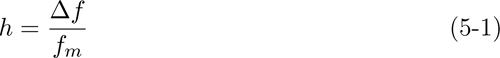
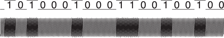
Figure 5–5. Frequency shift keying
The size of the deviation is called the modulation index h, where Δf is the maximum deviation from the carrier frequency, and fm is the highest frequency in the source signal being modulated onto the carrier. If the modulation index is greater than one, the carrier is varying in frequency more than the source signal, then the signal is called a wide-band transmission. If the modulation index is less than one, the carrier is varying in frequency less than the source, then the signal is called a narrow-band transmission. A modulation index of 0.5 is considered a very special value because this is the value used for minimum-shift keying, or MSK. MSK is a variant of FSK that is very spectrally efficient.
5.4. Frequency Band
Bluetooth low energy uses the 2.4GHz Industrial, Scientific, and Medical (ISM) band for transmitting information. This frequency band is very special for two reasons. Most radio spectrum is licensed, meaning you have to buy a license to transmit anything. For example, your local radio station might have lots of money to buy a license to transmit music and advertising, on the premise that the revenue from the sales of commercial spots is sufficient to pay for the music, wages, and license. Some frequency bands are licensed but at zero cost. This includes bands for aviation, military, and civilian emergency services. Some bands are free. Yes, free!
The 2.4GHz ISM band is one of the license-free frequency bands. You do not need to buy a license to transmit in this band as long as you follow the rules. The rules are very simple; the band must be used for a personal area network (PAN) or a local area network (LAN) with limited range and limited transmit power. The details of the rules themselves are very complicated; however, in essence, it is free to use for short-range applications.
The second reason the 2.4GHz ISM band is very special is that it is the only license-free spectrum that is the same in every country. This means that no matter where you buy a product that uses this band, you can use it in any other country without having to configure it. There are other ISM bands, such as those around 900MHz, but these use different frequencies and band sizes, depending on the locations; the United States uses 915MHz, whereas the European Union uses 868MHz. The 2.4GHz band, which is useable anywhere, extends from 2400MHz to 2483.5MHz. This gives a total available spectrum of about 83.5MHz.
5.5. Modulation
The Bluetooth low energy radio uses Gaussian frequency-shift keying. A Gaussian filter is one that optimizes the transition from one symbol to the next by increasing the time that is used to slide the frequency from one value to another. Without this filter, the frequency shift would be dramatically quick, causing much noise to be created. This means that when changing from a zero bit to a one bit, the transition is both fast and efficient.
When transmitting data, Bluetooth low energy transmits at one million bits per second (Mbps), with one bit per symbol. The modulation index is approximately 0.5, meaning that it is very close to the optimal MSK. The modulation index can vary between 0.45 and 0.55, meaning that Bluetooth low energy is not classified as an MSK radio; however, it has most of the MSK properties, including reducing side-band power output, which means less expensive filters are required to make it conform to the regulatory requirements.
To send a zero, a negative frequency deviation is used. To send a one, a positive frequency deviation is used. The minimum frequency deviation is about 180kHz. This means that if a center frequency of 2402MHz is used, a zero would be indicated by a transmission at 2401.820MHz, and a one would be indicated by a transmission at 2402.180MHz, as shown in Figure 5–6.

Figure 5–6. Modulation
5.6. Radio Channels
If you want to implement the most robust, longest-range system, it is always best to use more than one frequency to transmit information. Some systems achieve this by having very wide transmissions; 802.11, for example, uses either 20MHz- or 40MHz-wide channels to send data very quickly. Other systems do this by frequency hopping; Bluetooth classic uses 79 narrow channels that are all used when transmitting information. The choice is mostly arbitrary, except that many narrow channels will be able to find a way through complex multi-path environments that are constantly changing much more efficiently than fewer wide-band transmissions.
Figure 5–7 illustrates that Bluetooth low energy uses 40 radio channels to transmit information. The center frequency for each channel can be calculated very simply, as shown in Equation 5-2.

Figure 5–7. Radio channels
Here, fc is the center frequency of radio channel k.
This means that the lowest frequency used in Bluetooth low energy is 2402, and the highest frequency is 2480. At the bottom end of the frequency band, a gap of 2MHz is provided between a Bluetooth low energy channel and anything using the next frequency band below it. At the top end of the frequency band, a gap of 3.5MHz is provided between a Bluetooth low energy channel and anything using the next frequency band above it.
5.7. Transmit Power
In the 2.4GHz ISM band, there are limits to the maximum transmit power that a device can use to stay within the license-free regulations. For Bluetooth low energy, the specification limits the maximum transmit power to +10dBm. The LE specification also imposes that there is a minimum transmit power of –20dBm, so devices cannot be made so quiet that no other devices can hear them.
A + 10dBm transmit power means that it would be transmitted at 10mW, whereas at –20dBm, it would be transmitting at just 10μW.
5.8. Tolerance
All devices are manufactured with a given tolerance. Typically, the more accurate the tolerance, the more costly the devices. For the radio, the major tolerance that can be specified is the frequency accuracy. Even if a radio is designated to transmit around 2402MHz, it might actually be operating at 2401.850MHz or 2402.150MHz. This is the tolerance in the center frequency when transmitting a packet. In Bluetooth low energy, the center frequency tolerance is ±150kHz for the whole packet. The reason that the center frequency might be off is that it is typically obtained by multiplying the frequency from a known frequency crystal. This crystal would typically have a frequency of 16MHz; therefore, it must be multiplied by a factor of over 150 to get to up 2400MHz. Any inaccuracies in the crystal would be multiplied, as well, and included in the transmission frequencies. For example, if the crystal was actually outputting 16.0001MHz, the center frequency would be off by approximately 150kHz. This crystal would be said to have an error rate of 62 parts per million (ppm). Typically, low-cost, high-volume crystals with an error rate of approximately 50 ppm are readily available.
Another value that is very important is how much the radio drifts from its center frequency during the packet. This drift is caused by heat that builds up in a silicon chip during use. As the heat builds, the internal frequencies used in the radio will drift slightly. A Bluetooth low energy radio cannot drift more than 50kHz during a packet. This means that if the radio started transmitting perfectly at 2402.000MHz at the start of a packet, it would have to be between 2401.950MHz and 2402.050MHz at the end of the packet. There is also a maximum drift rate of 400Hz/μs.
5.9. Receiver Sensitivity
When building a receiver, there is really only one question that matters: How good is it? This is quantified by measuring the receiver sensitivity: how sensitive the radio is to detecting wireless transmissions from another device. This is measured in dBm, and is typically a very small number. The required receiver sensitivity for Bluetooth low energy is –70dBm. In other words, it has to be able to pick up 0.0000001mW of electromagnetic energy to be able to work. However, noise will always be present. There is no point in being able to detect a signal if you can’t decode it. Therefore, in practice, the sensitivity threshold is set at the value where a signal can be decoded with an acceptable bit error rate (BER). For Bluetooth low energy, this has been chosen as 0.1 percent BER.
Most controllers supporting Bluetooth low energy will have a receiver sensitivity of about –90dBm, or 1pW. This is an incredibly small amount of energy that is able to be detected from the noise of the band, but this leads to impressive ranges, as explained in the following section.
5.10. Range
To calculate the range of a Bluetooth low energy radio, the link budget of the system needs to be determined. The link budget is made up of a number of elements that use the power from the transmitter in a silicon chip before it is received by a peer silicon chip. These elements include the antenna and matching circuit gains and losses. However, assuming that the antenna and matching circuits make little difference,1 the main contributor to the link budget is the path loss. Path loss is a measure of how much the radio signal has reduced in power between the antenna in the transmitter and the antenna in the receiver. Equation 5-3 determines the path loss required for a given distance. Table 5–1 presents the correlation between path loss and distance; Figures 5–8 and 5–9 show the relationship graphically. It should be noted that this equation is an approximation, valid only for an isotropic antenna, and ignores any losses in the transmit/receive systems.
Table 5–1. The Relationship of Path Loss to Distance
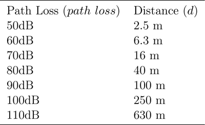
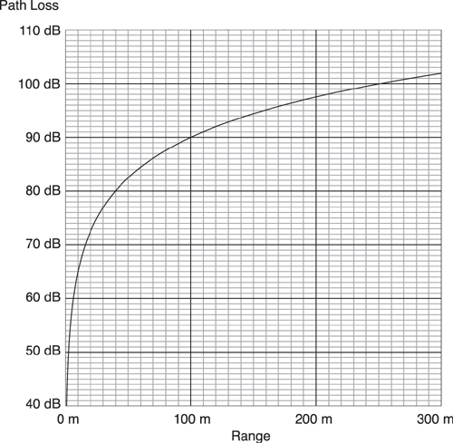
Figure 5–8. A graphic representation of path loss
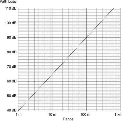
Figure 5–9. Path loss (log graph)
In the equation, d is the distance between the transmitter and the receiver.
When the transmit power is –20dBm and the receiver sensitivity is –70dBm, a path loss of 50dB, the range is 2.5 meters. This is the distance possible when the minimum transmit power is used, with the minimum receiver sensitivity.
When the transmit power is 0dBm and the receiver sensitivity is –80dBm, a path loss of 80dB, the range is 40 meters. This is the distance possible when a moderate transmit power is used, with a moderate receiver sensitivity.
When the transmit power is 10dBm and the receiver sensitivity is –90dBm, a path loss of 100dB, the range is 250 meters. This is the distance possible when the maximum transmit power is used with the receiver sensitivity possible with modern chips.