Chapter 7. The Link Layer

All this technology for connection and what we really only know more about is how anonymous we are in the grand scheme of things.

—Heather Donahue

The Link Layer defines how two devices can use a radio to transmit information between one another. This includes defining the detail of a packet, advertising, and data channels. It also defines procedures for discovering other devices, broadcasting data, making connections, managing connections, and ultimately sending data within connections. This is compounded by the challenges of wireless communication systems in the 2.4GHz ISM band, including interference, noise, and deep fades.

7.1. The Link Layer State Machine

Before we discuss packets and how they are used, it is important to understand the basic concept of the Link Layer state machine and its implications on the design of Bluetooth low energy.

As shown in Figure 7–1, the Link Layer state machine defines just five states:

• Standby

• Advertising

• Scanning

• Initiating

• Connection

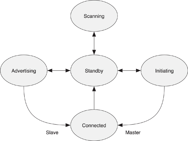
Figure 7–1. The Link Layer state machine

However, it should be considered that the scanning state has two substates: active scanning and passive scanning. The connection state also has two substates: master and slave.

Although the Link Layer state machine explains how devices can discover and connect to one another, it also explains another fundamental design decision that Bluetooth low energy implemented; the separation of the broadcast, discovery, and connection processes from the data transmitted in a connection. Part of this design was done for ultra-low power consumption on the part of the advertising devices. By reducing the number of advertising channels to just three, you can maintain robustness while reducing power consumption. But this requires separate advertising states and separate advertising packets. The Link Layer state machine has three states in which advertising packets are sent or received, and one state in which data packets are sent and received.

7.1.1. The Standby State

When Link Layers are powered on, they start in the standby state and remain there until the host layers tell them to do otherwise. It is possible to move from the standby state into either the advertising, scanning, or initiating states (see Figure 7–2). It is also possible to move into the standby state from every other state. The standby state is really the center—the most important, albeit inactive, state.

Figure 7–2. The standby state

7.1.2. The Advertising State

The advertising state (see Figure 7–3) allows the Link Layer to transmit advertising packets. It can also respond to scan requests from devices that are actively scanning by sending a scan response. The advertising state is required if a device wants to be discoverable or connectable. The advertising state is also required if a device wants to broadcast data to other devices in the area.

Figure 7–3. The advertising state

To be an advertiser, a device must have a transmitter, but it might have a receiver as well. A device that only supports the advertising state could be built with just a transmitter, saving the cost of the receiver on that chip. It should be noted that in practice the volume pricing for a dual-purpose chip with both a transmitter and a receiver might well end up being less expensive than a low-volume transmit-only chip.

It is possible to move from the advertising state into the standby state by stopping advertising. It is also possible to move from the advertising state into the connection state when an initiating device sends a connect request packet to this advertiser.

7.1.3. The Scanning State

In the scanning state (see Figure 7–4), a device will receive advertising channel packets. This could be used to simply listen to see what devices are advertising in the local area. Scanning is composed of two different substates: passive scanning and active scanning. Passive scanning only receives advertising packets. Active scanning also sends scan requests to advertising devices to obtain additional scan response data.

Figure 7–4. The scanning state

It is only possible to move from the scanning state into the standby state. This is done by stopping scanning.

7.1.3.1. Passive Scanning

In passive scanning, the device just passively scans, never transmitting anything. Passive scanning can therefore be implemented on a device that only has a receiver. By supporting only passive scanning, you can reduce the size and cost of the controller because there’s no need for a transmitter. But, as mentioned earlier, depending on the amount you’re producing, multi-purpose devices might end up costing less as a result of volume pricing.

7.1.3.2. Active Scanning

In active scanning, whenever a new device is discovered by the Link Layer, a scan request is sent to the advertising device, and a scan response is expected in reply. Both these scan requests and response packets are transmitted on the advertising channel. For active scanning to work efficiently, the data in the scan response must be mostly static because this data is expensive in terms of energy expended to retrieve due to the additional two packets that are transmitted or received. The data in the original advertising packet, however, can change regularly because this will always be received.

7.1.4. The Initiating State

To initiate a connection to another device, the Link Layer must first be placed into the initiating state. In the initiating state (see Figure 7–5), the receiver is used to listen for the device to which the initiator is attempting to connect. If an advertising packet from this device is received, the Link Layer will send a connect request to the advertiser and move into the connection state, in the assumption that the advertising device does the same. It is also possible to leave the initiating state to move back into the standby state by stopping initiating a connection.

Figure 7–5. The initiating state

7.1.5. The Connection State

The final state of the Link Layer state machine is the connection state (see Figure 7–6). This can be entered either via the advertising state or the initiating state. Both of these transitions are caused by an initiating device sending a connect request packet to an advertising device.

Figure 7–6. The connection state

Again, this has two substates: master or slave. In the connection state, data channel packets are sent and received between the two devices. This is the only state in which the data channels are used; all other states use the advertising channels. It is only possible to leave the connection state by moving into the standby state. This is done by terminating the connection.

7.1.5.1. The Master Substate

The master connection substate can only be entered from the initiating state. A device that becomes a master must initiate the connection to the peer device. When a device is a master, it must transmit packets to the slave at regular intervals. This provides the slave with opportunities to reply and send its own data.

7.1.5.2. The Slave Substate

The slave connection substate can only be entered from the advertising state. A device that becomes a slave must have been advertising to the peer device. When a device is a slave, it cannot transmit anything until a packet from the master is received correctly. Once a packet from its master is received, the slave can transmit a packet itself. If the slave wants to transmit more data, it must wait for the master to send another packet of data back to it. Slaves can save power by just ignoring the master at any time. By doing so, the slave device can save significant quantities of power by staying “asleep.”

7.1.6. Multiple State Machines

In an implementation of the Link Layer, it is possible to have multiple state machines; each state machine is separate. Using this configuration, a device can, for example, be a slave, advertise, and actively scan at the same time. Or, you could configure a device to be a master, advertise, passively scan, and initiate a connection at the same time, as illustrated in Figure 7–7. The device could also have multiple master connections to slaves at the same time.

Figure 7–7. An example of multiple state machines

Be aware that there are some restrictions related to deployment that are important to understand.

7.1.6.1. Not Master and Slave

The Link Layer is an “autocracy”; if a device is a master, it cannot also be a slave at the same time. Similarly, if a device is a slave, it cannot be a master at the same time. This implies that if a device is a master, it cannot advertise with a connectable advertising packet; however, it can still advertise with nonconnectable or discoverable advertising packets.

Consequently, if a device is already a slave, it cannot initiate a connection to another device because doing so could cause it to become the master of that device. By making this restriction, there will be no point in time when it is nondeterministic as to what the device should be doing.

The deterministic nature of the Link Layer enables Bluetooth low energy devices to be implemented using very efficient scheduling algorithms. Any nondeterministic system that is maintaining synchronization with multiple time domains will need to have very complex scheduling algorithms. These algorithms, by virtue of being nondeterministic, will also require significant processing requirements implemented in general-purpose CPUs. This does not fit in with the low-power goals for the technology. The deterministic design, therefore, allows for highly efficient algorithms that can be implemented by using discrete logic.

A device also cannot be a slave of two masters at the same time. If a device is a slave, it cannot advertise with a connectable advertising packet. Being a slave of two masters is actually a harder scenario than being a master and a slave at the time. In Bluetooth classic, this would be called scatternet. Bluetooth low energy does not support scatternets.

7.2. Packets

A packet is the fundamental building block of the Link Layer. A packet is really simple; it is a labeled piece of data that is transmitted by one device and received by one or more other devices. The label identifies the device that sent the data and which devices should listen to it.

Figure 7–8 shows the packet structure, which all packets share, regardless of what they’re used for. At the start of the packet is a short training sequence called the preamble. After that is an access address that is used by the receiver to distinguish this packet from the background radio noise. After the access address are header and length bytes. Immediately after these is the packet’s payload, followed by a cyclic redundancy check (CRC), which ensures that the payload is correct.

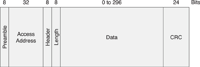
Figure 7–8. Packet structure

7.2.1. Advertising and Data Packets

In Bluetooth low energy, there are two types of packets: advertising and data packets. These packets are used for two completely different purposes. Devices use advertising packets to find and connect to other devices. Data packets are used once a connection has been made. The difference between advertising packets and data packets is that a data packet is understandable by only two devices, known as the master and slave devices; advertising packets, on the other hand, are sent by one device and can be either broadcast to any device listening or directed at a specific device.

Whether a packet is an advertising packet or a data packet is determined by the channel on which the packet is transmitted. There are 3 advertising channels and 37 data channels. If a packet is transmitted on one of the 3 advertising channels, then the packet is an advertising packet; otherwise, it is a data packet.

7.2.2. Whitening

The interesting thing about frequency-shift keying (FSK) receivers is their lack of ability to receive a very long sequence of bits of the same value. (To learn more about FSK receivers, go to Chapter 5, The Physical Layer.) For example, when transmitting a string of bits such as “000000000000”, the receiver will assume that the center frequency of the transmitter has moved to the left and it will therefore lose frequency lock. It then misses the next “1” bit and fails to receive the rest of the packet. To protect against this, a whitener is used to randomize the packets transmitted.

A whitener is typically a very short random number generator that outputs zeros and ones in a known order for a given packet (see Table 7–1). A receiver can then use the same random number generator to recover the original bits. To keep the original information in the output sequence, the original data is combined with the random number whitener using an exclusive-or operation.

Table 7–1. Using a Whitener in an Exclusive-Or Operation

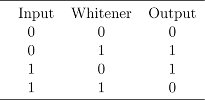
By using a random whitener combined with the original information in the packet, a string of identical bits in the original information will be converted into a sequence that is highly randomized. This reduces the chance that the receiver will lose frequency lock. If the long string of information bits were already random in nature, any further randomization will not hurt.

The whitening random number sequence is generated using a linear feedback shift register, similar to one used to calculate a CRC. The polynomial used is shown in Equation 7-1.

In this equation, x is the shift register.

The value of the shift register is initially set with the Link Layer channel number on which this packet will be transmitted, with the high bit set. This means that even if a packet is whitened on one channel that causes the receiver to lose lock, when it is transmitted on another channel, it will use a different whitening sequence, and therefore the receiver will be able to receive it. This is a very rare occurrence, but one from which the whitener allows recovery.

Table 7–2 shows how the whitener is used to stop long sequences of zeros or ones from being transmitted. This example shows the first 3 bytes of data being whitened when transmitted on channel 23. This means that the binary sequence:

input = 00000000 : 00100000 : 00010000

Table 7–2. Whitener LFSR: Input Bits and Resultant Output Bits

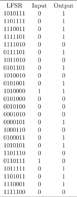
combined with the whitener of:

whitener = 11110101 : 01000010 : 11011110

is converted to:

output = 11110101 : 01100010 : 11001110

You can see that the data has become randomized with the whitener. The original input data has long sequences of single digits: 10,1,8,1,4. The output data does not have these long sequences, and critically, the longest single digit sequence is just four digits: 4,1,1,1,1,1,2,3,1,1,2,2,3,1.

7.3. Packet Structure

As shown in Figure 7–9, the packet structure is composed of a number of fields. Each of these fields is described in detail in the following subsections. Some fields contain multiple byte fields; therefore, the order of transmission of these bytes as well as the bits in these bytes also needs to be discussed.

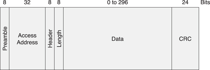
Figure 7–9. Packet structure

7.3.1. Bit Order and Bytes

Packets are transmitted bit by bit, but they are composed of bytes of data. When these bytes of data are transmitted, they are transmitted with the least significant bit first. Therefore 0x80 is transmitted as 00000001, whereas 0x01 is transmitted as 10000000. Most multiple-byte fields are transmitted least significant octet first. Therefore, the value 0x010203 would be transmitted as the following:

11000000010000001000000

7.3.2. The Preamble

The first 8 bits of a packet that are transmitted are either a 01010101 or 10101010 sequence. This is a very simple alternating sequence by which a receiver can set its automatic gain control and also determine the frequencies being used for the zero and one bits.

The reason that this sequence is very important is due to the possible range of input signal strengths with which a chip must be able to cope. The radio must be able to handle a signal at –10dBm at the antenna, all the way to –90dBm. This is a dynamic range of 80dBm. From a receiver’s perspective, this means that it could receive a packet with a power of 1pW or a power of 0.1mW. An automatic gain control would therefore have to detect the input power level and adjust its gain to bring the signal into a range with which the controller can easily work.

The determination of whether the preamble is 01010101 or 10101010 is determined by the first bit of the access address that is transmitted. If the first bit of the access address is a “0”, the 01010101 sequence is used. If the first bit of the access address is a “1”, the 10101010 sequence is used. This always guarantees that the first 9 bits of a packet have alternating bits: either 101010101 or 010101010.

7.3.3. Access Address

The next 32 bits of a packet are the access address. This can be one of two types:

• Advertising access address

• Data access address

The advertising access address is used when broadcasting data or when advertising, scanning, or initiating connections. The data access address is used in a connection after a connection has been established between two devices.

When a controller wants to receive a packet, it always knows which access address it will be receiving. As the receiver is turned on and tuned into the correct frequency, the receiver will start to receive bits of data. Even if no other device is around transmitting at this time, the radio will pick up background radiation. Given simple probabilities of receiving pure random noise, the chance of receiving a sequence of bits that matches the preamble is fairly high; typically, once every few minutes for a low-energy device with its receiver constantly open. Therefore, the access address is used to reduce the probability of random noise causing a pseudo-packet to be received.

The Link Layer also doesn’t know when the other device will be transmitting packets, so it has to keep a copy of all the possible bits that have been received for the last 40μs and check each time a new bit is shifted into this register to see if this sequence of bits now matches the expected preamble and access address. This process is called correlation of the access address.

For advertising channels, the access address is a fixed value: 0x8E89BED6. In binary this is transmitted from left to right as the following:

01101011011111011001000101110001

This means that for an advertising packet the preamble would be 01010101. This value was chosen because it has excellent correlation properties. The fixed value means that any Bluetooth low energy device can correlate against this access address and know it is receiving an advertising packet, even though it might never have received a packet from this specific device before.

For data channels, the access address is a different random number on each and every connection between two devices. This random number, however, must adhere to a number of rules, primarily to ensure that the access address still has good whiteness.

As is explained in Section 7.2.2 on whitening, it is necessary to whiten radio transmissions to ensure that receivers can be built as easily as possible. The most basic rule is that there cannot be more than six zeros or ones anywhere in the access address. The packet also has to be different from the advertising access address by at least 1 bit. Also, the access address cannot have any repeating patterns; each octet of the access address must be different. There should be no more than 24 bit transitions, stopping the use of an alternating bit sequence. Finally, there must be at least 2 bit transitions in the last 6 bits, to ensure that just before the header starts that there are bit transitions, just in case the header whitens to a long sequence of bits.

Given the preceding rules, it can be shown that there are approximately 2³¹ possible uniquely valid random access addresses. Or in other words, it is possible to have approximately 2 billion Bluetooth low energy devices within range of one another, talking at the same time. That was probably a slight design overkill, but remember Bluetooth low energy has been designed for success. Another useful feature of this random access address for data channels is that an attacker cannot determine which two devices are in a connection by just receiving this access address. This ensures the privacy of devices during a connection.

7.3.4. Header

The next part of a packet is the header. The contents of the header depends on whether the packet is an advertising packet or a data packet.

For the advertising packet (see Figure 7–10), the header includes the advertising packet type as well as some flag bits to specify whether the packet includes public or random addresses. There are seven advertising packet types, each having a different payload format and a different behavior:

• ADV_IND—General advertising indication

• ADV_DIRECT_IND—Direct connection indication

• ADV_NONCONN_IND—Nonconnectable indication

• ADV_SCAN_IND—Scannable indication

• SCAN_REQ—Active scanning request

• SCAN_RSP—Active scanning response

• CONNECT_REQ—Connection request

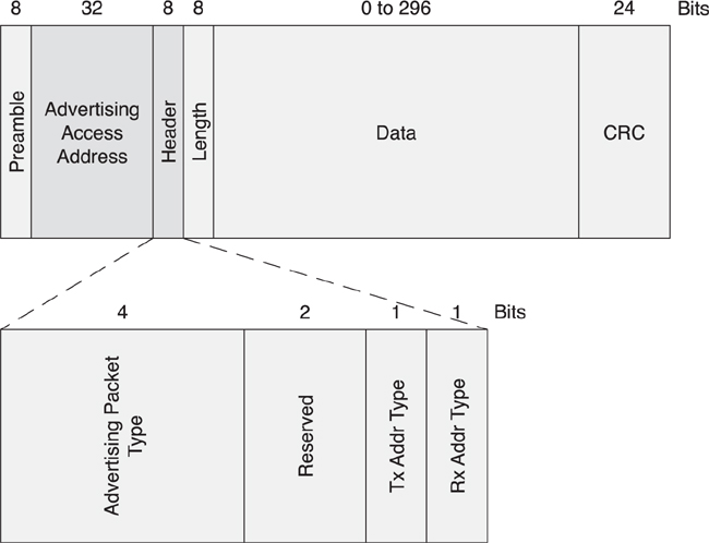
Figure 7–10. The contents of an advertising packet header

Figure 7–11 illustrates the header for data packets, which includes bits to enable the reliable delivery of packets, manage low power, and route the payload into either the local controller or to the host.

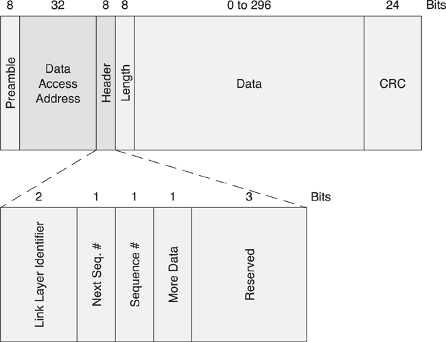
Figure 7–11. The contents of a data packet header

7.3.5. Length

For advertising packets, the length field comprises 6 bits, with valid values from 6 to 37. For data packets, it’s 5 bits in length with valid values from 0 to 31. After the length field is the payload, which contains the same number of bytes of data as the value in the length field.

It might appear strange that the length field is a different length for advertising packets and data packets. The main reason for this is a design decision that accomodates 31 bytes of useful data in an advertising packet. However, an advertising packet’s payload also always includes a 6-octet address for the advertising device. Adding the 6 octets of this address with the 31 octets of useful advertising data resulted in a packet length of 37 octets, and thus the requirement for a 6-bit length field.

Data packets are much easier. The size of data packets is less critical; most data being transferred is just a few octets in length, and therefore an absolutely maximal-sized packet was never considered useful. It’s also interesting to note at this point that if the packet is encrypted, it includes a 4-octet message integrity check value, shortening the actual data in the payload to just 27 octets. To keep the design of the Link Layer as simple as possible, unencrypted packets are not allowed to be longer than this 27-octet limit; this reduces the complexity of buffering within the Link Layer.

7.3.6. Payload

The payload is the actual “real” data that is being transmitted. It could be advertising data about the device or service data that is being broadcast to devices in the local area. It could be additional active scan response data such as the device name and the services it implements. It could be information required to establish a connection or to maintain the connection once it is established. It could also be the application data that is being transmitted from one device to another.

7.3.7. Cyclic Redundancy Check

The last part of every packet is a 3-byte cyclic redundancy check (CRC). This CRC is calculated over the header, length, and payload fields. The CRC is a 24-bit CRC that is strong enough to detect all odd numbers of bit errors as well as 2- and 4-bit errors. This means that all 1, 2, 3, 4, 5, 7, 9, and so on, bit errors are detected in all packets.

The choice of a 24-bit CRC might appear strange, considering that most wireless standards use 16- or 32-bit CRCs. However, for the size of packet that Bluetooth low energy can send, a 32-bit CRC would not be able to detect 6-bit errors any more reliably than the 24-bit CRC used, and therefore would simply waste 8 microseconds of radio activity for every packet. If the length of the header, length, and payload fields were increased past the maximum of 39 bytes, it would be necessary to increase the CRC size to be able to detect even 4-bit errors. A 16-bit CRC, however, is not strong enough to detect the 4-bit errors over all possible 336 bits of the payload and CRC that are being protected. The 24-bit CRC is consequently the best compromise between robustness and power saving.

The polynomial used for the 24-bit CRC is as demonstrated in Equation 7-2:

7.4. Channels

As described in Section 5.6 of Chapter 5, The Physical Layer, Bluetooth low energy uses 40 channels. The Bluetooth low energy channels differ from classic channels because of the relaxed modulation index. This means that the radio energy for each channel is spread wider; therefore, to prevent interference between adjacent Bluetooth low-energy channels, they are separated by 2MHz, instead of the classic 1MHz.

In the Link Layer, these channels are divided into two types: advertising channels and data channels. These channel types are aligned with the advertising packets and data packets, as described earlier. When a packet is transmitted, if the packet is sent on an advertising channel, it is an advertising packet. If the packet is sent on a data channel, it is a data packet.

There are 3 advertising channels and 37 data channels, as shown in Figure 7–12 (the advertising channels are rendered in darker shading). The 3 advertising channels are not all placed in the same part of the ISM band because that would mean that any deep fade in a single part of the band would stop all advertising. Instead, the advertising channels are placed a minimum of 24MHz apart from one another.

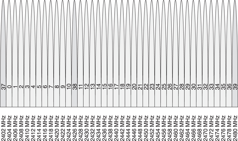
Figure 7–12. The Link Layer channel map

The advertising channels are placed strategically away from significant interferers such as a Wi-Fi access point. These access points typically use one of three 802.11 channels, either channel 1, channel 6, or channel 11. These channels have center frequencies of 2412MHz, 2437MHz, and 2462MHz and a width of approximately 20MHz. This means that channel 1 extends from 2402MHz to 2422MHz, channel 6 extends from 2427MHz to 2447MHz, and channel 11 extends from 2452MHz to 2472MHz.

The advertising channels are placed at 2402MHz, 2426MHz, and 2480MHz. This means that the first advertising channel is below Wi-Fi channel 1, the second advertising channel is between Wi-Fi channel 1 and channel 6, and the third advertising channel is above Wi-Fi channel 11. This is illustrated in Figure 7–13, in which 3 Wi-Fi channels have blocked the use of data channels 0 to 8, 11 to 20, and 34 to 32. The 3 advertising channels, 37, 38, and 39, are all interference free.

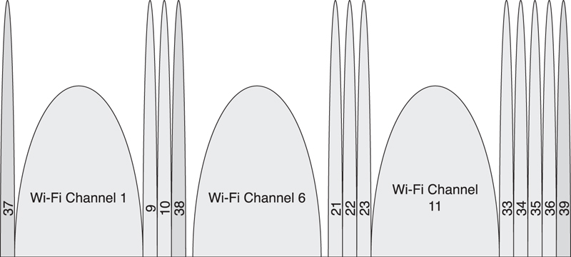
Figure 7–13. Link Layer channels and Wi-Fi channel coexistence

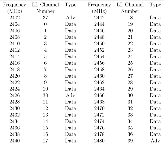
The data channels are placed every 2MHz between the advertising channels. Table 7–3 shows the complete list of advertising and data channels, the Link Layer channel number, and the center frequency.

Table 7–3. Complete List of Advertising and Data Channels, the Link Layer

The advertising channels are numbered from 37 to 39; the data channels are numbered from 0 to 36. The separation of the data channel and advertising channel numbers is so that the frequency-hopping algorithm is very easy to implement.

7.4.1. Frequency Hopping

When in a data connection, a frequency-hopping algorithm is used. Because the number of data channels is 37, which is a prime number, the hopping algorithm is very simple, as demonstrated in Equation 7-3:

The hop value is a value that can range from 5 to 16; it is added onto the last frequency modulo 37 every time the frequency-hopping algorithm is used. This means that every frequency will be used with equal priority, regardless of the hop value. In Figure 7–14, the channels chosen, given a hop value of 13, are shown over time. Also, the algorithm can be implemented by just adding the hop value, comparing the value with 36, and if it is greater than this, subtracting 37. No divisions, multiplications, or other complex mathematics are required.

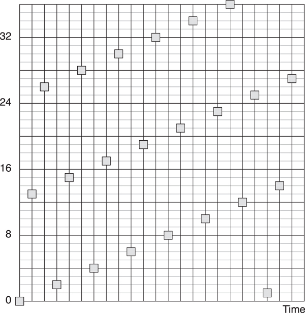
Figure 7–14. Frequency hopping of data channels over time

7.4.2. Adaptive Frequency Hopping

Adaptive frequency hopping makes it possible for a given packet to be remapped from a known bad channel to a known good channel so that the interference from other devices is reduced. To do this, a channel map of good and bad channels is kept in both devices. If the channel that would have been chosen by using Equation 7-3 is a good channel, then that channel is used; if the channel that would have been chosen is a bad channel, then it is remapped onto the set of good channels, as depicted in Figure 7–15. A minimum of two data channels must be marked as good by a master.

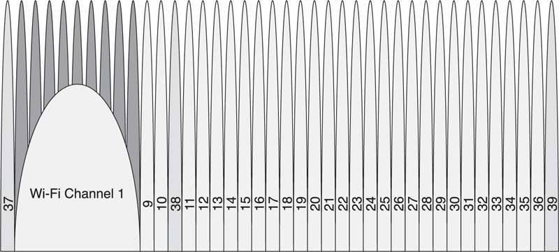
Figure 7–15. Link Layer adaptive frequency-hopping bad channels with Wi-Fi channel 1

Suppose, for example, that a Bluetooth low energy device is in the same area as a Wi-Fi channel 1 access point that is streaming data to another Wi-Fi device. The Bluetooth low energy device would mark Link Layer data channels 0 to 8 as bad channels. This means that when the two devices are communicating, they would cycle through the channels and remap these channels to a set of good channels, as shown in Table 7–4 and Figure 7–16.

Table 7–4. An Example of Adaptive Frequency Channel Remapping

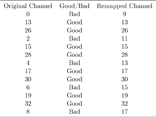
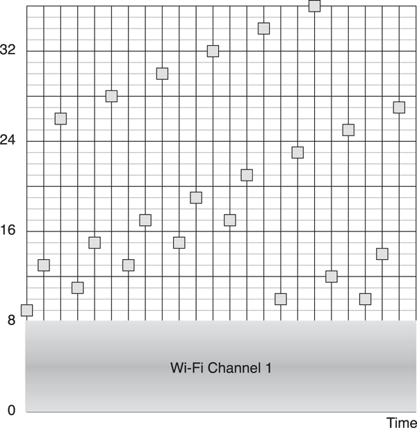
Figure 7–16. Adaptive frequency-hopping remapping

This remapping of channels ensures that even in the face of heavy interference, Bluetooth low energy will still continue to send data. It also enables the device to react very quickly to new interference. In Bluetooth classic, most controllers can react to a new interferer within just a few seconds, after which both will readily coexist without any concerns.

To assist in the remapping process, the host can inform the controller of the current channel conditions. This information could come directly from the interfering radio in the device or it could come from something much more exotic. Most Blue-tooth controllers can also perform passive band scanning to determine the location and extent of interference and act on this without any input from the host.

7.5. Finding Devices

A device uses the advertising channel to find another device, with one device advertising and another device scanning, as illustrated in Figure 7–17. There are four types of advertising that can be performed by devices: general, directed, nonconnectable, and discoverable.

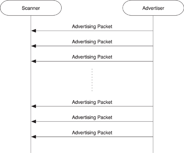
Figure 7–17. An advertiser sending advertising packets

Each time a device advertises, it transmits the same packet in each of the three advertising channels; this sequence of packets is called an advertising event. Apart from directed advertising, all of these advertising events can be sent as often as every 20 milliseconds to as infrequently as every 10.28 seconds. Typically, a device that is advertising would advertise once per second. The time between advertising events is called the advertising interval. The host can control this interval.

However, there would be a problem if devices advertised periodically because as their clocks drifted independently, two devices would constantly be advertising at exactly the same time, possibly for a long period of time. To prevent this from happening, all advertising events, except directed advertising, are perturbed in time. This perturbation is done by adding a random addition time from the last advertising event of somewhere between 0 and 10 milliseconds. This means that even if two devices collide on the same advertising channel at the same time and share the same advertising interval, they will probably not collide the next time they send an advertising event.

Scanning is important to complete the picture for low-energy advertising. Scanning is required to be able to receive advertising events. How much time is available and how quickly a device needs to find another device will determine the time that will be dedicated to scanning. For example, if the user is directly touching an interface that is looking for devices, the device would scan continuously for a number of seconds, soaking up all the devices that are advertising in the area.

However, if the user is just walking around, the scanning device might only be scanning for a few milliseconds every second, or for a few hundred milliseconds every minute, looking for interesting information, depending on whether the user just arrived home, sat down in a café, or perhaps walked into a meeting room. This background scanning can then change the behavior of the device depending on where it is; if you are in the café, the phone might automatically switch to silent mode; at home, it might direct all phone calls through to the home phone system; in an office meeting room, all calls might go to your voicemail along with a message to the caller indicating that you are in a meeting and cannot be disturbed.

7.5.1. General Advertising

General advertising is the most general-purpose advertising type. A device that is generally advertising can be scanned by a scanning device or go into a connection as a slave when it receives a connect request. General advertising can be sent by a device that has no other connections; in other words, it is not a slave to another device or a master of another device.

7.5.2. Direct Advertising

Sometimes a device needs to make a connection with another device quickly. For a slave to do this, it must advertise. To allow for the fastest possible connection times, direct advertising events are used. These packets contain two addresses: the advertiser’s address and the initiator’s address. An initiating device that receives a direct advertising packet addressed to itself immediately sends a connect request packet in response.

These directed advertising events also have special timing requirements. The complete advertising event must be repeated every 3.75 milliseconds. This timing allows a scanning device to scan for just 3.75 milliseconds and pick up directed advertising devices.

The problem with sending packets this quickly is that the advertising channels will become congested with directed advertising packets, resulting in all other devices in the area not being able to advertise themselves. For this reason, directed advertising is not allowed to continue for more than 1.28 seconds. The controller will automatically stop the advertising if the host hasn’t already done so or if a connection has not been established. Once the 1.28 seconds have expired, the host would then just be able to use general advertising at a much lower duty cycle to allow the device to still be connectable.

When using directed advertising, a device cannot be actively scanned. Also, directed advertising packets cannot have any additional data in the payload of the packet; they contain only the two addresses needed, and nothing more.

7.5.3. Nonconnectable Advertising

Devices that don’t want to be connectable use nonconnectable advertising events. Typical uses of this include devices that are broadcasting data and have no intention of being either scannable or connectable. This is the only type of advertising that a device equipped with only a transmitter can use.

A nonconnectable advertising device will never enter the connection state; therefore, it can only transition between the advertising state and the standby state when asked to do so by the host.

7.5.4. Discoverable Advertising

The final type of advertising event is the discoverable advertising event. This cannot be used to initiate a connection, but it can be used to allow another device to scan the advertising device. This means that the device is discoverable, both for advertising data and scan response data, but cannot be connectable. This is an advanced form of broadcast data, whereby the dynamic data can be included in the advertising data, whereas static data would be included in the scan response data.

Discoverable advertising will never enter the connection state; instead, it moves back to the standby state when it is stopped.

7.6. Broadcasting

As explained in the previous section, devices can advertise. However, for a device to be considered a broadcasting device, it must also include some useful data in that advertisement. This means that you can broadcast with three of the four advertising events: general advertising, nonconnectable advertising, and discoverable advertising.

When broadcasting, the data is labeled within the advertising packets. This is done because not all devices will understand all possible broadcast data. As such, there needs to be a way for the broadcast data to be both labeled and sized. Each piece of data starts with a length field that indicates the length of the following type and data fields. Next is a type field that a receiver will use to determine if it understands the following data (see Chapter 12, The Generic Access Profile, Section 12.5). By using this “length : type : data” format, devices that do not understand a particular type of data can skip over it because they know the size of the data and can therefore continue with the next piece of data.

Broadcast data can be received by any passive or active scanning devices nearby. Broadcast data cannot be acknowledged. A broadcasting device also doesn’t know if any device received its data or if any device is attempting to listen to the data. Therefore, broadcasting must be considered to be an unreliable operation.

7.7. Creating Connections

If the data transfers are more complex than can be performed by broadcasting the data, or the data needs to be reliably delivered to another device, a connection will be required. A connection uses the data channels to reliably send information, in two directions, between two devices. It uses adaptive frequency hopping to be robust and a very low duty cycle to keep the power consumption as small as possible.

As illustrated in Figure 7–18, the first step in creating a connection is for one device to advertise by using a connectable advertising event and for another device to initiate a connection to the advertising device. To make a connection, either the general advertising event or the direct advertising event types must be transmitted by the advertiser. When the initiator receives the advertising packet from the correct device, it sends a connect request back to the advertiser. This connection request packet includes everything that is needed at the start of the connection, which is presented in the following list:

• Access Address to be used in the connection

• CRC initialization value

• Transmit window size

• Transmit window offset

• Connection interval

• Slave latency

• Supervision timeout

• Adaptive frequency-hopping channel map

• Frequency-hop algorithm increment

• Sleep clock accuracy

Figure 7–18. Creating connections with which two devices can reliably transmit data

Once the connect request packet is sent or received, the devices are connected and data packets can be exchanged.

7.7.1. Access Address

The master always determines the access address that will be used in the connection. The value is random, adhering to a few rules, as detailed in Section 7.3.3. If the master has multiple slaves, it will choose a different random access address for each slave. The randomness of this value ensures that the probability for collisions between different masters and slaves is very low. The randomness also enhances privacy by not allowing a scanner to determine which two devices are communicating.

7.7.2. CRC Initialization

The CRC initialization value is another random value chosen by the master. This is random because a small probability exists that two masters in the same area could use the same access address to talk to different slaves. If this did occur, the slaves could receive interfering data from the wrong master. By randomizing the CRC initialization value for each slave, the probability of having two masters and slaves with the same access address and the same CRC initialization value is very small.

7.7.3. Transmit Window

Advertising is always done based on the timing of the slave. The slave is the device that needs to save the most power, so this is the correct design decision. However, if the master device is already doing something else, possibly something more important, it must interleave the Bluetooth low energy activity around its other traffic. During connection setup, this information is conveyed in two parameters: window size and window interval.

The transmit window starts after the end of the connection request packet, plus an additional mandatory delay of 1.25 milliseconds, plus the transmit window offset. The transmit window offset can have any value from 0 to the connection interval, in multiples of 1.25 milliseconds. At the start of the transmit window, the slave device opens up its receiver and waits for a packet to come from the master. If this packet is not received within transmit window size, the slave aborts and tries again one connection interval later.

The most interesting thing about the connection process is that once the connection request has been transmitted, the master believes it has a connection; the connection has been created but not proven to have been established. Once the slave receives the connection request, it believes it is also in a connection; again, the connection has been created but not proven to have been established.

In the interests of efficiency, the host is notified immediately when the connection is created. The connection might not succeed, the slave might not receive the connection request, or the two devices might be such a long distance apart that the connection has a high probability of failure. However, because the host is notified of the connection being created, it can start to send data down into the controller, ready for it to send in the very first packet over the air, saving time and therefore energy. Because the first data packet is not sent until after the mandatory 1.25-millisecond delay that follows the creation of the connection and the host stack notification, the host stack should have sufficient time to provide this data into the controller, using the very first opportunity to send data. This mandatory delay also provides any batteries with time to recover from the possibly exhausting advertising procedure before the connection is created.

The connection is only considered established once a packet has been acknowledged. Establishment doesn’t change how the connection works, but it does change the link supervision timeout, from just six connection timeouts, to the value in the connection request message. This ensures that if the connection is not established quickly, it is terminated immediately.

7.7.4. Connection Events

When in a connection, the master has to transmit a packet to the slave once every connection event. A connection event is the start of a group of data packets that are sent from the master to the slave and back again. A connection event is always conducted on a single frequency, with each packet transmitted 150 microseconds after the end of the last packet.

The connection interval determines how frequently the master will talk to the slave; it is the time between the start of the last connection event and the start of the next connection event. This can be any period from 7.5 milliseconds to 4 seconds in multiples of 1.25 milliseconds. To determine how infrequently the slave is allowed to talk to the master, the slave latency is used. This is a multiple of the connection interval and therefore determines how many times the slave can ignore the master before it is forced to listen. It should be noted, however, that this must still be quicker than the supervision timeout.

As illustrated in Figure 7–19, each connection event is a connection interval apart. Each connection event starts with a single packet from the master, and can continue until either the master or slave device stops responding. The times between connection events contain no packets from the master to this slave or the other way around.

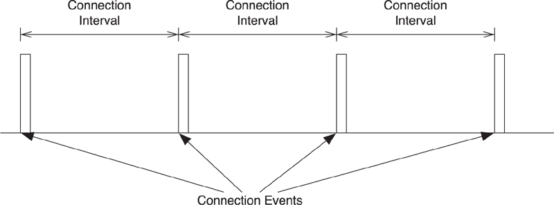
Figure 7–19. Connection events

For example, if the connection interval is 100 milliseconds and the slave latency is 9, the slave can ignore the master for 9 connection events but is forced to listen for the 10th, or once every second. The supervision timeout, therefore, must be a minimum of 1010 milliseconds. At the extreme end, the maximum supervision timeout is 32 seconds, and, therefore, with a connection interval of 100 milliseconds, the slave latency must be 319 or less.

However, it is not a good idea to give the slave just one opportunity to listen for the master within the supervision timeout when the slave is using its slave latency to the maximum. Thus, it is recommended that the slave is given six opportunities to listen. Therefore, in the preceding example, if the connection interval is 100 milliseconds and the slave latency is 9, the supervision timeout should be a minimum of 6 seconds, allowing the slave to listen a minimum of six times before the link is dropped.

7.7.5. Channel Map

The adaptive frequency-hopping channel map is a bit mask of the data channels that are known to be good or bad. Because there are 37 data channels, the channel map is 37 bits in length. If the bit is set to one, the channel is a good channel and will be used for data traffic. If the bit is zero, the channel is a bad channel and will never be used for data traffic.

The frequency-hopping algorithm’s hop value is a random number between 5 and 16. It is used in the frequency-hopping algorithm before the adaptive remapping algorithm is used, as described in the frequency-hopping Section 7.4.1. The number zero is obviously not allowed because this could mean that the frequency would never change.

Very low hop numbers are not desirable because most interferers are typically more than a couple of megahertz in width; therefore, having a very small number would not move the next transmission opportunity away from the interferer quickly enough, causing continued interference. The same logic is used for values 17 and higher. With a hop increment of 17, for example, every other frequency used would be just 3 channels away because of the modulo 37 operations used in the frequency-hopping algorithm (refer to Equation 7-3).

7.7.6. Sleep Clock Accuracy

Finally, the sleep clock accuracy value is sent from the master to the slave. This value determines the range of accuracies that the clock is able to guarantee. If the clock is timed from a crystal, the crystal will have a known accuracy over the temperature range, from, for example, 20ppm at room temperature to 50ppm at or . Therefore, the clock accuracy would have to state that this device has a clock accuracy of up to 50ppm.

The clock accuracy is used to determine the uncertainty window of the slave device at a connection event. If the slave has not synchronized its timing with that of the master for 1 second, and both devices have a timing accuracy of 500ppm, then the combined uncertainty of 1,000ppm has to be multiplied with the time away, to give a 1 millisecond uncertainty window. This means that the slave must wake up 1 millisecond early and stay on for an extra 1 millisecond, just in case the master and slave clocks have both drifted at the maximum ppm in different directions.

Having more accurate clocks can help save power. For example, if the crystals used in two devices were, for instance, 150ppm in one device and 50ppm in another, then the combined accuracy would be just 200ppm. So, after one second away, the slave would have to wake up just 200 microseconds early and stay on for an extra 200 microseconds. If a device is waking up infrequently, this could run for 5 times longer than the two devices with 500ppm crystals. It is therefore recommended that high-accuracy crystals be used in devices that have very low-power requirements and need to maintain a connection for some time.

7.8. Sending Data

Once in a connection, devices can send data to one another. This is done by sending data packets at connection events. Data packets are distinct from advertising packets because they are private communications between two devices rather than broadcast communications to any device that is listening. The biggest differences between advertising packets and data packets are the length of the payload that is possible and the packet header.

The length of the payload in a data packet can be anywhere from 0 octets in length to 31 octets. A zero-length payload in a data packet is an empty packet; it has no application data but can still include some information from the packet header. The maximum length payload (at 31 octets) is smaller than the advertising packet’s maximum length. It is also only possible to have this large a packet if it is encrypted.

An unencrypted data packet has a maximum of just 27 octets of data in it to allow for the retransmission of a data packet, even after encryption has been established between the data packet being sent into the controller and encryption being enabled in the controller.

7.8.1. Data Header

The data packet header, as shown in Figure 7–20, contains just the following four fields:

• Logical link identifier (LLID)

• Sequence number (SN)

• Next expected sequence number (NESN)

• More data (MD)

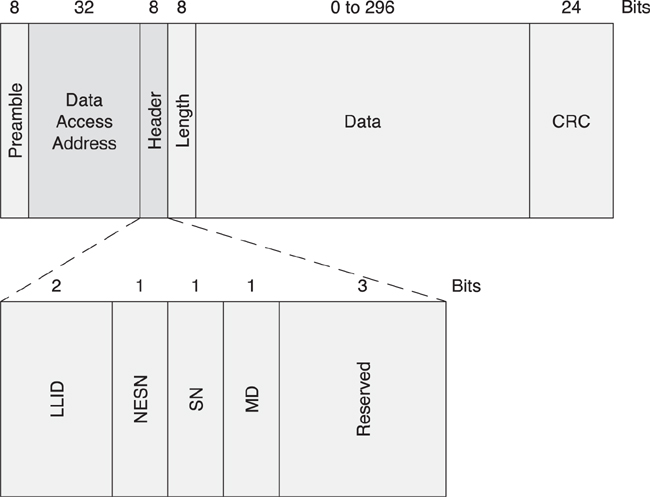
Figure 7–20. The data packet header

There is no “packet is encrypted” bit because this is a modal property of the connection, just like for the adaptive frequency hopping or the connection event intervals.

7.8.2. Logical Link Identifier

The logical link identifier (LLID) is used to determine if the packet contains one of the following types of data:

• Link Layer control packet (11)—This is used for managing the connection

• Start of a higher-layer packet (10)—Or for a complete packet

• Continuation of a higher-layer packet (01)

If the packet is a Link Layer control packet, this is indicated by the logical link identifier, and this data is passed directly to the Link Layer control entity. The meaning of the data within this packet is therefore determined by the Link Layer control entity, as described in Section 7.10.

All other packets are to or from the host. The host is able to send packets larger than the maximum 27 octets of data that can be included in a single Link Layer data packet; therefore, it is able to segment these. To do this, the packet is labeled as either a start of a higher layer data packet or a continuation of a higher layer data packet. This is illustrated in Figure 7–21, in which a very long higher layer data packet is split over three Link Layer data packets. The first data packet is labeled with an LLID of “start”, whereas the other two data packets are labeled with an LLID of “continuation”.

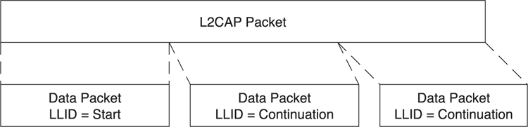
Figure 7–21. Packet fragmentation

This is interesting from two standpoints. First, the Link Layer doesn’t require knowledge of the ultimate size of the packet at the start of the packet. It is possible to send start, continuation, continuation, ... continuation, continuation, before sending another start message. The number of continuation messages is not fixed at the start of the message.

This allows the second interesting side effect: it is possible to always send zero-length continuation messages without any impact on the higher layer data. This allows empty packets to always be sent, meaning that simple acknowledgement messages can always be sent as zero-length continuation messages. These zero-length continuation packets are known as empty packets.

7.8.3. Sequence Numbers

To enable the reliable transfer of data, all data packets have sequence numbers. The sequence number for each new data packet sent is different from the last data packet’s sequence number, with the first packet in a connection having a sequence number of zero. This allows a receiving device to determine if the next packet that is received is a retransmission of the previous packet because the sequence number is the same or a transmission of a new packet because the sequence number is different.

In data packets, there is a single bit for the sequence number, starting at zero for the first data packet that is sent. The sequence number then alternates between one and zero for each new data packet that is sent by a device.

7.8.4. Acknowledgement

To perform acknowledgement of a data packet, a single bit is used. This is called the next expected sequence number bit. This informs the receiving device of the next sequence number that the transmitting device is expecting it to send.

If the packet received by a device has the sequence number zero, the next expected sequence number that it receives must be one; otherwise, the packet would have been retransmitted. Therefore, it’s possible to signal if the packet received was received correctly or if the packet needs to be retransmitted. This is illustrated in Figure 7–22.

Figure 7–22. Sequence numbers

7.8.5. More Data

The final bit in the data channel packet header is the more data bit. This signals to the peer device that the transmitting device has more data ready to be sent. The peer receiving device upon seeing the more data bit set in a received packet should continue to communicate in this connection event. This automatically extends connection events while there is still data to be sent. It also quickly closes connection events for which there is no more data to be sent. The more data bit also allows a device that needs to save power to close the connection event gracefully and quickly by setting its more data bit to zero. The more data bit can therefore be used to enable lots of data to be reliably delivered in a very efficient manner by using as few transmitted packets as possible.

7.8.6. Examples of the Use of Sequence Numbers and More Data

The processing of sequence numbers, next expected sequence numbers, and more data bits is shown in Figure 7–22 and described in the following:

1. The master transmits its first packet by using the default sequence number of zero and the next expected sequence number of zero. The master also sets the more data bit because it has two packets of data to send (SN_master=0, NESN_master=0, MD_master=1). This packet was received correctly by the slave; therefore, the slave’s next expected sequence number is updated (NESN_slave=1).

2. The slave’s first packet (SN_slave=0) was transmitted with the newly updated next expected sequence number (NESN_slave=1). This packet also has the more data bit set (MD_slave=1) because the slave is about to send some interesting data. This packet was not received by the master, so the master’s next expected sequence number was not changed. The slave continues to listen to the master because the more data bits for both the master and the slave were set.

3. The master’s second transmission (SN_master=0, NESN_master=0, MD_master =1) is a retransmission of its first packet. The master never received a packet from the slave and therefore must retransmit its packet. The slave receives this packet and detects that this is a retransmission of the last packet it received because the sequence number is identical; thus, the slave does not update its next expected sequence number. The slave sees that the master has more data to send to it, so it continues this connection event by transmitting another packet.

4. The slave retransmits its first packet (SN_slave=0, NESN_slave=1, MD_slave=1). The master receives this packet successfully and updates its next expected sequence number (NESN_master=1). The master sees that the slave has more data to send and continues this connection event by transmitting another packet.

5. The master’s third transmission is a new packet requiring a new sequence number (SN_master=1, NESN_master=1, MD_master=0). This packet contains the last of the data the master has to send, so the master has set the more data bit to zero. The slave receives this packet successfully and updates its next expected sequence number (NESN_slave=0). The slave still has more data it wants to send, so it continues the connection event.

6. The slave’s third transmission is a new packet requiring a new sequence number (SN_slave=1, NESN_slave=0, MD_slave=0). The slave’s more data bit has been set to zero to indicate that it doesn’t have any more data to send. The master receives this packet correctly and updates the next expected sequence number (NESN_master=0). Because the last packets of the master and slave both indicated that neither device has any more data, the connection event is immediately closed.

7. Some time later, the master wakes up at the next connection event and transmits a new packet to the slave with a new sequence number and the latest next expected sequence number (SN_master=0, NESN_master=0, MD_master=0). This packet also lazily acknowledges the last packet from the slave. The slave receives this packet successfully and updates its next expected sequence number (NESN_slave=1). The slave has no more data to send but needs to respond with an empty packet.

8. The slave’s fourth transmission is an empty packet using a new sequence number (SN_slave=0, NESN_slave=1, MD_slave=0). The slave also has no more data to send; therefore, it sets its mode data bit to zero. The master receives this packet successfully and updates its next expected sequence number (NESN_master=1). Because the last packets of the master and slave both indicated that neither device has any more data, the connection event is immediately closed.

As the preceding example illustrates, the sequence number and next expected sequence number are always in lock-step with one another. This ensures that packets are always reliably delivered and in order. A packet is not considered to be received when the CRC fails to verify that the contents of the packet have been received correctly.

It is also possible to enable flow control by using the next expected sequence number. If a device does not have enough buffer space to process a message at a given time, it is not able to update the next expected sequence number. This forces the other device to retransmit this message, effectively pushing the buffering requirements onto the sending device and away from the receiving device.

There is one other effect of this whole process on connection events. If a packet is not successfully received because a few bit errors cause the CRC to fail, and this happens again on the same packet within a single connection event, the two devices will stop using that connection event. The devices will then resynchronize at the next connection event and try again. This means that if a given channel is being blocked due to interference, then very quickly the two devices will discover this interference and stop using that channel. By moving to a new channel quickly, the interference caused by transmitting on the blocked channel is mitigated almost immediately, but data is still delivered to the other device very quickly at the next connection event.

7.9. Encryption

When in a connection, data within the payload can be encrypted. This encryption can ensure confidentiality of the data against attackers. Confidentiality means that a third party cannot intercept the messages, decipher them, and read the original contents of the messages because the “attacker” does not have the shared secret used to encrypt the link.

Encrypted packets also include a message integrity check value that ensures the data is authenticated. Authentication means that the validity of the sender can be confirmed by calculating a signature of the encrypted data with a shared secret. This prevents a third party from changing any of the bits in the packet. Authentication allows the receiver of a message to know that the data packet it has just received was sent by a device it trusts. A personal identification number (PIN) used to authenticate bank card holders is a classic example of authentication; the PIN verifies that the authorized person is using the bank card.

Encrypted packets also include a packet counter to stop replay attacks. A replay attack is one in which an attacker intercepts a given message and then at a later date replays this message in the hope that it will result in a response. For example, without replay attack protection, it could be possible to scan for lots of packets being transmitted by a device and then replay these packets and see what happens. If the receiving device was a sewage valve near a city park, the results could be “interesting.” Clearly, protecting against replay attacks is something very important.

7.9.1. AES

All encryption and authentication in Bluetooth low energy is built around a single encryption engine called the Advanced Encryption System (AES). This encryption engine was originally designed as part of a United States government program to find a suitable encryption engine for the future. It has since been adopted by many wired and wireless standards and has so far held up well against the attempts by security researchers to find weaknesses in its algorithms.

AES can be built in multiple forms, typically determined by the size of the blocks of data and keys that it can process at any given time. In Bluetooth low energy, the 128-bit key size and 128-bit data blocks are used. This means that all keys are 128 bits in length, and up to 16 octets of encrypted data can be created at a time.

The AES encryption block is very simple: it takes two inputs and generates one output. The two inputs are a 128-bit key value and a 128-bit block of plain-text data, and the output is a 128-bit block of encrypted data. The reason the two inputs are labeled as key and plain-text data is that the key must be processed first before being used in the encryption block, whereas the plain text is immediately processed by the encryption block. Therefore, it is more efficient to set up the key once and then pass in different plain-text blocks and encrypt them quickly than it is to use a different key for each block.

Thus, the encryption of some data, plaintext, with a key, key, using an algorithm, E, to produce encrypted text, ciphertext, can be represented by using the function in Equation 7-4:

In Bluetooth low energy, the AES encryption engine is used for four basic functions:

• Encrypting payload data

• Calculating a message integrity check value

• Signing data

• Generating private addresses

The signing of data is defined by the Security Manager, and the generating of private addresses is defined by the Generic Access Profile.

7.9.2. Encrypting Payload Data

To encrypt the payload data, the payload is split into 16-byte blocks, and for each block a cipher bit stream is generated. This cipher bit stream is then Exclusive-Or’ed with the plain text. This is defined by using the standard IETF RFC 3610. This standard defines a method for encryption and authentication using Counter with Cipher Block Chaining-Message Authentication Code Mode or CCM.¹ This is a standard encryption algorithm for any size key and any size message.

In Bluetooth low energy, the A_x encryption blocks are used. These are initialized plain-text blocks that have a known format and include a nonce composed of a packet counter, a direction bit, and an initialization vector (IV). In the equation that follows, the || notation means concatenation.

nonce = Packet Counter || Direction || IV

The packet counter is a 39-bit value that is incremented for each new non-empty packet that is transmitted. The packet counter always starts with zero when encryption is enabled. Empty packets are not encrypted; therefore, they do not need to increment the packet counter. The initialization vector is a random value that is 64 bits in length, where 32 bits of this vector are contributed by each device in the encrypted link (see Section 7.10.3). Therefore, the nonce is 13 bytes in length.

The other octets of the A_x are per the CCM specification. The first octet is a flags field that will always be set to 0x01 to indicate that this is an A_x block. The last two octets are the block counter. The block counter is set to 0x0001 when used to encrypt the first 16 octets of the payload (C_Block1) and to 0x0002 when used to encrypt the second 11 octets of the payload (C_Block2). The CCM specification is also used to encrypt the message integrity check value (M_MIC), and for this, the block counter is set to 0x0000.

C_MIC = E_key(0x01 || nonce || 0x0000)

C_Block1 = E_key(0x01 || nonce || 0x0001)

C_Block2 = E_key(0x01 || nonce || 0x0002)

The cipher blocks are then Exclusive-Or’d with the various parts of the message to generate the encrypted payload.

encrypted = C_Block1 ⊕ Block1 || C_Block2 ⊕ Block2 || C_MIC ⊕ MIC

This encrypted payload is then sent to the peer device. Because the peer device knows the shared secret—the key value—it can decrypt the message by using the same packet counter, direction, and IV values. When the encrypted payload is sent, the CRC is calculated over the encrypted payload, not the original payload blocks. The header and length fields of the data packet are never encrypted.

7.9.3. Message Integrity Check

The message integrity check (MIC) value is used to authenticate the sender of the data packet, and this MIC is inserted between the Data and the CRC, as illustrated in Figure 7–23. This ensures that the encrypted packet is sent by the peer device and not by a third-party attacker. To calculate the MIC, the AES encryption engine is used again. This time, the output of one block is used as the input to the next block, chaining together the blocks to ensure that every bit in the original message is as important as every other bit in calculating the MIC.

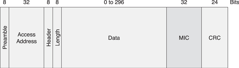
Figure 7–23. The encrypted data format

To calculate the MIC, the same nonce is used for encrypting the payload. Three or four B blocks are used. The first B₀ block contains the nonce and the original length of the data being authenticated. This length field comprises 16 bits, even though the maximum size of the payload that can be authenticated in low energy is just 27 octets.

B₀ = 0x49 || nonce || length

The next B₁ block contains additional data that should be authenticated with the payload but is not contained within the payload. In Bluetooth low energy, this is used to authenticate some of the bits in the header of the packet. The only bits that need to be authenticated are the logical link identifier bits. All other bits in the header are masked to zero; this simplifies calculation and allows precalculation of blocks without having to know values such as SN or NESN, and so on because these bits are not important from a security point of view.

B₁ = 0x0001 || header_masked || 0x00000000000000000000000000

The next block or two contains the actual payload data being authenticated. B₂ contains the payload data from octets 0 to 15. B₃ contains the payload data from octets 16 to 26.

To calculate the MIC, these blocks are then chained together by using a single key as used for encrypting the payload. Only the most significant 32 bits of the payload are used in the packet.

X₀ = E_key(B₀)

X₁ = E_key(X₀ ⊕ B₁)

X₂ = E_key(X₁ ⊕ B₂) where B₂ = Payload_[0..127]

MIC = E_key(X₂ ⊕ B₃)_[128..96] where B₃ = Payload_[128..215]

When an encrypted packet is received, the same MIC calculation is performed on the receiving device to check that the MIC value computes to the same, given the same inputs. If the value does not compute correctly, the connection is immediately disconnected. No further communication will occur, and the peer device will automatically eventually enter supervision timeout. This appears at first glance to be a very drastic approach; however, the MIC will not even be checked if the CRC fails—the packet will just be rejected and a new packet retransmitted from the peer.

The only way that an MIC can fail is if an attacker is currently attempting to attack the link or if a number of bit errors were falsely accepted by the CRC, causing the MIC to fail. In the first case, the safest approach is to immediately disconnect the link because it might already be compromised. In the second case, the data contained in the packet is already compromised because the CRC has falsely identified it as a correct packet. So again, the safest approach is to assume the worst and disconnect the link. Once the connection has been dropped, the two devices can quickly reconnect, establish a new initialization vector, and reencrypt the link. The approach of reestablishing a new initialization vector refreshes the nonce and, therefore, the encryption that is used on the connection.

It is also possible to reestablish a new initialization vector while in a connection, if needed. Given that the packet counter has a fixed size, and that the encryption is only considered secure if nonce values are never repeated, it is necessary to refresh the initialization vector periodically. This will not occur very frequently; there are a total of 2³⁹ – 1 packets that can be sent in a connection before the nonce would repeat, which would take over 12 years of continuously transmitting packets to get anywhere close to wrapping. However, Bluetooth low energy has been designed for success and for connections to be stable for many years. As such, it is already a defined process to refresh the nonce. To do this, a new initialization vector is generated by using the encryption pause and resume procedures, as defined in Section 7.10.4.

7.10. Managing Connections

Once two devices are in a connection, they can send and receive data and manage the connection. Connection management involves sending Link Layer control messages. There are only seven Link Layer control procedures:

• Updating the connection parameters

• Changing the adaptive frequency-hopping channel map

• Encrypting the link

• Reencrypting the link

• Exchanging feature bits

• Exchanging version information

• Terminating the link

7.10.1. Connection Parameter Update

When the connection is created, the connection parameters are sent in the connection request packet, as detailed in Section 7.7. After a connection has been active for a period of time, the connection parameters might no longer be suitable for the services being used over this connection. The connection parameters will need to be updated for the services to be used efficiently. Instead of disconnecting the link and then reconnecting it with different connection parameters, it is possible to do a connection parameter update within the link, as illustrated in Figure 7–24.

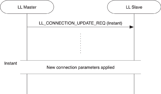
Figure 7–24. Performing a connection update procedure

To do this, the master sends a connection update request to the slave with the new parameters by using LL_CONNECTION_UPDATE_REQ. There is no negotiation of these parameters; the slave must use them. If the slave doesn’t accept the parameters being suggested, it only has one option available to it: disconnect the link. The connection update request includes a subset of parameters that were used in the connection request message sent earlier during connection creation and one additional parameter, called the instant:

• Transmit window size

• Transmit window offset

• Connection interval

• Slave latency

• Supervision timeout

• Instant

The instant is the parameter that determines from when the connection update will start. When the master sends the message, it picks a time in the future when the connection update will be actioned and includes it in the message. The slave, upon receiving the message, will remember this instant future time and then wait until the specified time before moving to the new connection parameters. This helps solve one of the largest problems in wireless systems: packet retransmission. As long as the packet is retransmitted enough times and eventually gets through before the instant passes, the procedure will work well. If, however, the packet does not get through in time, the link will probably drop.

Given that Bluetooth low energy has no clock, the only way to determine an instant is to count connection events. Therefore, each connection event is counted, with zero being the first connection event in the link; the one that was transmitted in the first transmit window after the connection request. The instant, therefore, is the connection event count at which the new parameters will be used. The master should provide enough opportunity for the slave to receive this packet. Even at maximum latency, this should typically allow at least six attempts for the message to be sent by the master to the slave. If the slave latency is 500 milliseconds, then the instant would typically be placed at least 3 seconds in the future.

Once the instant arrives, the slave listens for the transmit window, just like during connection creation. This allows the master to shift the timing of the slaves, both within the 1.25-millisecond slot but also at the gross level. This better allows the master device that is also a Bluetooth classic device to align its own Bluetooth low energy slaves to those of its other activities. Once this procedure is complete, a new connection interval, supervision timeout, and slave latency values are used.

7.10.2. Adaptive Frequency Hopping

Adaptive frequency hopping is very important for the successful survival of any radio technology in an open wireless band. Unfortunately, some technologies don’t perform adaptive frequency hopping and are therefore susceptible to interference. The biggest problem with adaptive frequency hopping, especially in model devices, is that the set of channels at any given time that can be considered good or bad can be considered to be constantly changing. This means that there needs to be signaling to allow devices to change this channel map. This procedure is shown in Figure 7–25.

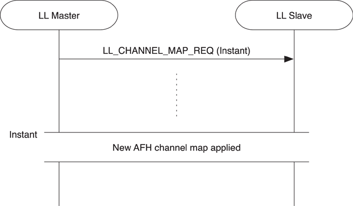
Figure 7–25. The Channel map update procedure

The adaptive frequency-hopping updates are sent in a channel map request packet LL_CHANNEL_MAP_REQ. This is sent from the master to the slave and includes only the following two parameters:

• New channel map

• Instant

The instant is the same concept as the instant used in the connection update. It determines a point in time that the new channel map will be used. At the instant, and afterward, the new channel map is used for all connection events in the future at least until the next time the channel map is updated.

The channel map is a 37-bit field that has one bit for each data channel. If a given channel’s bit is set to one, the channel is considered good and will be used; if a given channel’s bit is set to zero, the channel is considered bad and will not be used.

The channel update request can only be sent again after the instant has passed. This places a restriction on how fast the connection’s channel map can be updated. Typically, the channel map would be updated only when the connection is performing poorly using its current set of channels or when the host determines that the current bad channels are now good again. No Link Layer control procedures are provided to allow a slave device to change the channel map or even notify its master of its own channel conditions.

7.10.3. Starting Encryption

To start encryption, the link must be unencrypted. To encrypt the link, both the nonce and a session key (SK) need to be created. The nonce requires 4 octets of information to be contributed by each device, and the session key requires 8 octets of information to be contributed by each device. An additional key is also required, called the long-term key (LTK). This is the shared secret that is established during pairing (for more information, go to Chapter 11, Security, Section 11.2).

To start encryption, as illustrated in Figure 7–26, the master first transmits an encryption request message (LL_ENC_REQ) to the slave. The slave then responds with an encryption response message (LL_ENC_RSP). The encryption request packet from the master includes its 4-byte contribution to the initialization vector, 8 bytes of session key diversifier, and some additional information that the slave transmitted to it when they initially paired. This additional information is static for a given master, and the slave can use this information to determine with which master it is communicating and possibly derive the LTK for the master from this information. By doing this, the slave might not need to store any information about bonded devices. The encryption response packet from the slave includes its 4-byte contribution to the initialization vector and its contribution to the session key diversifier.

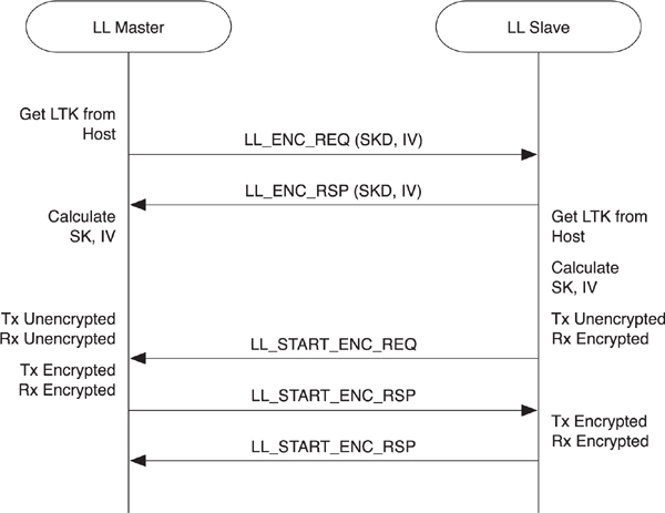
Figure 7–26. Starting the encryption procedure

If the LTK is not available on the slave side, the slave will then immediately send a reject indication to the master along with the reason it rejected the encryption. If the LTK is available, the slave will start a three-way handshake to begin encryption. The three-way handshake is required because the slave, for example, must be able to transmit an unencrypted packet to the master, but it must be able to receive an encrypted packet back. Thus, this handshake procedure moves the two devices in lockstep into a fully encrypted link.

When encryption is started, a session key is used to encrypt the link. The session key is calculated from the LTK and the session key diversifier contributed to by both devices.

The session key diversifier enables an LTK to be used multiple times. This is done by ensuring that each time a connection is encrypted a different encryption key is derived from the session key. The master and slave contribute half of this diversifier to ensure that even if one device is an attacker, the other device can force a different diversifier and therefore a different encryption key. The primary reason all this is done is to protect against the single weakness in AES: A key cannot be used more than once, ever. Therefore, even though we have a shared secret, LTK, we cannot use this to encrypt the application data. Instead, we must diversify this LTK into a session key, SK.

The two session key diversifiers (SKD), SKD_master contributed by the master, and SKD_slave contributed by the slave, are concatenated together and used as the plaintext input into the AES encryption engine (refer to Equation 7-4). The LT K is used as the key input into the AES encryption engine. The output of the AES encryption engine is the session key that is used as the key to encrypt the link.

SK = E_LTK (SKD_master || SKD_slave)

The initialization vector (IV) is also calculated from the two values contributed by both devices IV_master contributed by the master and IV_slave contributed by the slave by concatenating them together.

IV = IV_master || IV_slave

All data transfers are paused while encryption is starting. This is done on the master before it sends its encryption request packet; on the slave, it’s done before it sends its encryption response packet. This ensures that no data can be sent unencrypted while the encryption is starting up; it also helps the three-way handshake to perform correctly.

Once the SK and IV have been calculated by the slave, the slave sends the start encryption request packet (LL_START_ENC_REQ) unencrypted, but the slave sets to receive an encrypted packet by using the SK and IV values just calculated. If the master doesn’t receive the slave’s packet, the master will respond by requesting the same packet again, using an empty packet because all other data packets have been paused. Because empty packets can never be encrypted (there is no payload to encrypt), the slave can receive either this packet or the master’s next encrypted packet.

The master responds to the slave’s packet by sending an encrypted packet (LL_START_RSP) that uses the same SK and IV values it has just calculated and setting up to receive an encrypted packet in response. The slave can receive this encrypted packet because it was configured to receive encrypted packets. The slave will now turn on encrypted packet transmission.

Upon receipt of this master’s encrypted packet, the slave will respond with an encrypted packet (LL_START_RSP). The master can receive this encrypted packet because it has already turned on the reception of encrypted packets.

Once the master has received this final packet, it can turn on the flow of application data, all of which will be encrypted. Once the slave has received the Link Layer acknowledgement of this final packet, it can turn on the flow of application data, all of which will be encrypted.

On Bluetooth classic, authentication must be performed before encryption can be started. This costs both in terms of time and additional messages that need to be transmitted. In Bluetooth low energy, this process is not necessary because each packet that is transmitted includes authentication. Therefore, the authentication of the link is done on each and every packet, not just once at the start of the encryption process.

7.10.4. Restarting Encryption

Restarting encryption is useful to refresh the session key and is used to encrypt the link when the packet counter has almost expired or because a new link key has been established, and the host wants to use this new link key to derive the session key. It is not a procedure that will be used very often; in fact, some devices might never have a connection up long enough and so never require the restarting of encryption.

To restart encryption, the same starting encryption process is used, but only after encryption is paused. Pausing encryption means that application data is paused and then encryption is turned off. This ensures that no application data can be sent unencrypted while encryption is restarting. It is effectively a two-step process: The master must first pause encryption and then restart it by using the starting encryption procedure.

The pausing of encryption is another three-way handshake, but in the opposite order to the way that the starting encryption handshake is carried out.

As illustrated in Figure 7–27, the master sends a pause encryption request packet (LL_PAUSE_ENC_REQ) to the slave, after the master’s application data is paused.

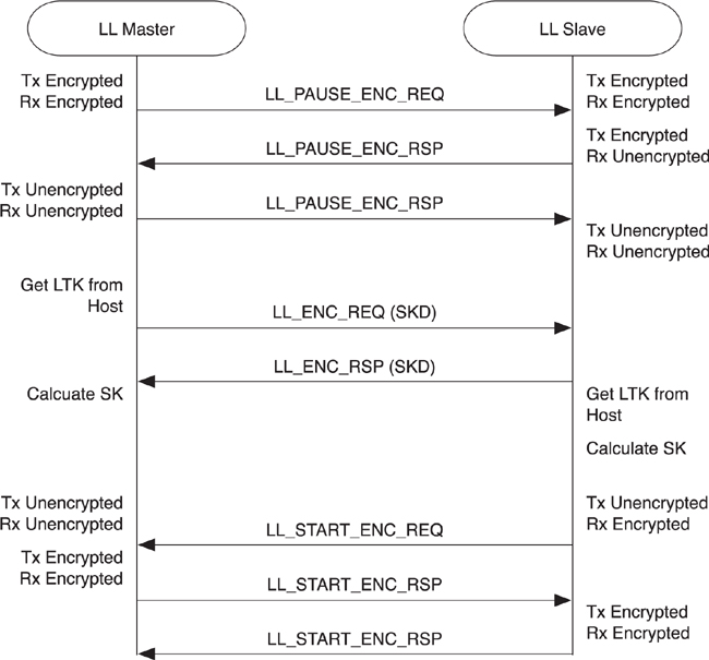
Figure 7–27. Restarting the encryption procedure

Upon receipt of the pause encryption request packet from the master, the slave will pause its application data and then send a pause encryption response packet (LL_PAUSE_ENC_RSP) and disable the reception of encrypted packets; the master will only be able to send empty packets to acknowledge any packets the slave might send.

After it has received this slave pause encryption response packet, the master will turn off the transmission and reception of encrypted packets and reply with another pause encryption response packet (LL_PAUSE_ENC_RSP). The slave can receive this packet because it has already disabled encryption. Once the slave receives this packet, it will also disable encryption for transmitted packets.

Encryption is now disabled. No application data can be sent because all application data has been paused. This protects against the possibility of sensitive application data being sent unencrypted.

Once encryption has been disabled, the master will immediately send the encryption request packet (LL_ENC_REQ) to the slave to initiate the starting encryption procedure defined in the last section.

7.10.5. Version Exchange

Sometimes it is useful for debugging purposes to find out a little more about a device than just its device address and what information is available in the host and application layers. Version information is only useful for debugging purposes and can be obtained from devices by the Link Layer autonomously or by the host requesting the information, as shown in Figure 7–28. The version information cannot be used for changing the behavior of the device; therefore, it does not need to be exchanged on every new connection. However, most devices will request this information once every 10 or more connections so that a sniffer can pick this information up and help with the debugging of the connection.

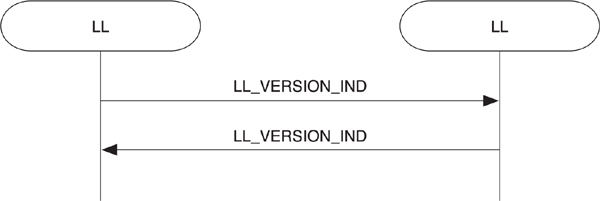
Figure 7–28. The version exchange procedure

This autonomous behavior of the Link Layer troubles some people. Why would a Link Layer want to receive version information every 10 connections? Simply, when you have a problem with two devices that need debugging, you might not have any ability to trigger a version information exchange from a host in either of these devices. Therefore, to be able to characterize these devices, a version information exchange that occurs infrequently is much better than nothing at all.

The classic example here is a device that is paired with only one other device (so no other device can connect and request this version information) that does not exhibit the buggy behavior for many months after being initially paired, and now that device is exhibiting buggy behavior. Having these version exchanges autonomously sent by the Link Layer every few connections will help tremendously in solving this problem now, and not in a few months’ time.

Version information includes the following:

• Version number

• Company identifier

• Sub-version number

The version number is a number assigned to a given published version of the Blue-tooth specification with which this device is compliant.

The company identifier is an assigned number from the Bluetooth Special Interest Group (SIG) that is allocated to the company that manufactured this controller.

The sub-version number is a number assigned by the company that manufactured the controller; it must be different for each implementation or revision of the controller. There is no defined way to assign this number, and if debugging of a device is important, then the manufacturer of the device should be contacted directly. The device manufacturer contact details are typically exchanged at UnPlugFest events, where engineers test and validate these controllers before shipping them in mass volume. This contact information is also available in the qualification database for all shipping products.

To exchange version information, either device can send a version information indication packet, if they have not already done so during the current active connection. If a device receives a version information indication from a peer device and it has not already sent its own message, it will respond with a version information indication packet. After this has completed once, the procedure cannot be requested again. This information is static and therefore will not change while in a connection. So, it’s pointless to ask again for the same static information. The controller should cache this information while the connection is active in case the host asks for it again.

7.10.6. Feature Exchange

The feature information is used by a peer device to determine what a device can do. It exposes the set of optional features supported by a device. As illustrated in Figure 7–29, this information can be requested by the master by using the feature request packet (LL_FEATURE_REQ) at most once, if at all, during any connection. Upon receipt of the master’s request, the slave replies with the feature response packet (LL_FEATURE_RSP). This information does not need to be exchanged to attempt to use an optional feature because all features must be enabled, and all optional features have a way to reject this request. For example, if encryption is not supported or enabled, then a reject indication packet is returned, safely rejecting the encryption request.

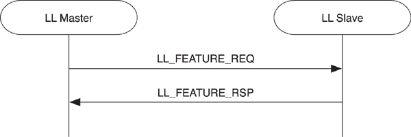
Figure 7–29. The feature exchange procedure

In the first version of Bluetooth low energy, there is only one feature bit defined: encryption supported. This states that encryption is supported by a device.

7.10.7. Terminating Connections

The only other Link Layer control procedure that can be performed is the termination procedure. This, unsurprisingly, disconnects the link and moves both the master and slave connections back into standby state. A link can be terminated at any time, by either device, for any reason, as shown in Figure 7–30.

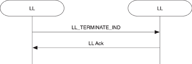
Figure 7–30. The terminate procedure

To terminate the link, a device sends a terminate indication packet (LL_TERMINATE_IND). It then waits for the acknowledgement of this packet at the Link Layer, after which it disconnects. If a device sends the terminate indication packet but does not receive any acknowledgement of this packet, the sending device will just timeout this procedure and the connection will still be disconnected. This timeout is the same as the supervision timeout value.

As soon as a device receives the terminate indication packet, in response it sends an empty packet to immediately acknowledge this packet, and then it disconnects.

Connections can also be terminated for two other reasons:

• Supervision timeout

• MIC Failure

When these other reasons are encountered, there is no terminate indication packet sent; the link is just disconnected, and the hosts on both sides are notified accordingly.

7.11. Robustness

To be robust, the Link Layer uses two very strong algorithms to ensure that data gets through without interference and that when data is sent from one host, it is delivered to a peer host unchanged.

7.11.1. Adaptive Frequency Hopping

Adaptive frequency hopping is essential for the efficient movement of data between devices communicating by using the 2.4GHz ISM band. There are so many different devices using this band that having technology that protects against interference is essential. Adaptive frequency hopping was originally brought into the Bluetooth classic specification in late 2003; it brought in a step change in performance improvements when compared with pre-2003 devices.

Simply put, adaptive frequency hopping is a way of taking a frequency-hopping radio and masking out bad channels by remapping them onto good channels. To do this, both devices have a channel map. This channel map is 37 bits in length, with each bit mapping directly onto a given Link Layer channel. Bit 0 in the channel map is related to the Link Layer channel 0; bit 1 in the channel map is for Link Layer channel 1; bit 36 in the channel map is related to the Link Layer channel 36. If a channel’s bit is set to one, the channel is a used channel; if a channel’s bit is set to zero, the channel is an unused channel. A minimum of 2 bits must be set as used into this channel map.

Take, for example, the channel map if all three main Wi-Fi channels are actively being used. These are channels centered at 2412MHz, 2437MHz, and 2462MHz. This means that only 9 Link Layer channels would be considered good: 9, 10, 21, 22, 23, 33, 34, 35, and 36. Three values define the channel map, ChannelMap is transferred between devices, Used is the set of good channels from the ChannelMap, and numUsed is the number of these good channels. These values for the preceding example would therefore be as follows:

ChannelMap = 0001111000000000111000000000011000000000₂

Used = [9, 10, 21, 22, 23, 33, 34, 35, 36]

numUsed = 9

If a connection were set up with this channel map, sent in the connect request packet from the master to the slave, with the hop interval set to 7, the preadaptive frequency-hopping channels used for this connection would be calculated by using the frequency-hopping equation, as shown in Figure 7–5, and as explained in Section 7.4.1.

The adaptation of these channels occurs after the initial frequency f_n is calculated.

The first connection event on the link should be channel 7. This is not in the set of good channels, so it would be remapped into the set of good channels. To do this, the set of good channels, Used, is ordered by channel number, and the unmapped channel number is mapped into this by modulating this with the number of good channels, numUsed: in this case, we have 9 good channels. The seventh good channel, Link Layer channel 35, is used as the channel in the connection event.

Used[7 mod numUsed ] ⇒ 35

At the next connection event, the channel would be calculated from the last unmapped channel.

f_n+1 = (f_n + hop) mod 37

f_n+1 = (7 + 7) mod 37

(7 + 7) mod 37 = 14 mod 37 ⇒ 14

Channel 14 is also an unused channel, so this is again remapped into the Used channels.

Used[14 mod numUsed ] = Used [5] ⇒ 33

At the next connection event, the channel would be calculated again from the last unmapped channel:

(14 + 7) mod 37 = 21 mod 37 ⇒ 21

Channel 21 is in the set of used channels, so this is just used directly.

As you can see in Table 7–5, this can continue for each connection event in the future.

Table 7–5. Remapping Channels by Using Adaptive Frequency Hopping

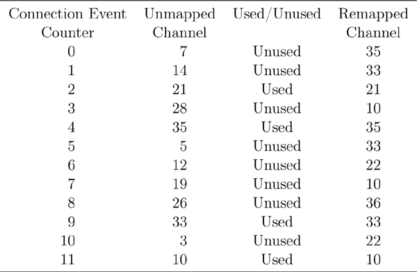
By using adaptive frequency hopping, data can always be transferred, even if lots of interferers are in the area, by remapping channels that are marked as unused to used channels that are known to be good.

7.11.2. Strong CRCs

The size of the CRC value in Bluetooth low energy is 50 percent larger than the size of the CRC in Bluetooth classic and most other wireless short-range devices. Unfortunately, Bluetooth classic has proven that a 16-bit CRC is not strong enough for the 2.4GHz ISM band. This was solved by adding another 16-bit CRC in the Logical Link Control and Adaptation Protocol Layer (L2CAP) to ensure that even if the CRC protecting data in the controller passed a packet up to L2CAP that has bit errors that were not protected, the host can still protect against these bit errors by using this second CRC. Unfortunately, this makes every L2CAP packet much larger, and for resource-constrained devices, the complexities of calculating a CRC in software also complicate the implementation.

Because of the experience gained from Bluetooth classic, Bluetooth low energy uses a much stronger CRC at the controller. This CRC is a 24-bit value that protects the packet. This CRC will detect all single-bit, two-bit, three-bit, four-bit, and fivebit errors, and all other odd numbers of bit errors in the packet. This is much stronger than a 16-bit CRC, and when compared with much larger packets used in wired protocols such as Internet Protocol (IP), it provides the same strength. This is because the packets in low energy are much shorter; thus, a shorter CRC can provide an equivalent level of protection.

The other problem that Bluetooth classic has is that the header of its packets is protected by a relatively weak header error-check value, which is just an 8-bit CRC. Obviously, if this falsely identified a packet, the main CRC should also fail.

Again, this experience has shown that having a separate header error check and main packet CRC does not help much. If the packet is good, then the controller still has to run two separate LFSRs, one for the header and one for the payload. If the packet is bad, the probability of the error occurring in the header is relatively low; the whole packet will probably have to be received anyway, which will not result in the expected power savings by using a separate header error check in the first place.

Bluetooth low energy takes an alternate design choice. It uses a single strong CRC that protects against the header, length, and payload fields of the packet, including any encrypted packets’ message integrity check value. This means that the full strength of the strong CRC is used over the complete packet, except for the preamble and access address; both of which must be received bit for bit perfect for the packet to be received in the first place. This is not only more robust but equally efficient.

And by having just one CRC—as compared to the three used in Bluetooth classic—the system is also simpler to implement. This shows why designing all layers in the specification at the same time is the best way to create a top-to-bottom, high-quality specification that can meet the market requirements.

7.12. Optimizations for Low Power

The following sections discuss how Bluetooth low energy has been optimized for ultra-low power consumption. The primary methods include the following:

• Keeping the packets short

• Using a high physical bit rate

• Providing low overhead

• Optimized acknowledgement scheme

• Single-channel connection events

• Subrating connection events

• Using offline encryption

Power consumption can be measured in multiple ways, but here it will be considered that two types of power consumption are critical to low power consumption within a device. First, low peak-power consumption is essential to allow a device to be powered from low-cost button-cell batteries. If the peak power is too high, the batteries would burn out too quickly, significantly reducing the lifetime of the device. Second, low power-per-application-bit is essential to allow a device to be used for a long time, sending a certain quantity of application data.

7.12.1. Short Packets

One of the exceptionally complicated parts of wireless technology is the actual radio that is used. Most of these radios are built by using bulk CMOS² technology. This creates a dilemma for designers because to make the radio stable, they need to increase the cost by adding circuitry to keep the frequency stable. Bluetooth low energy solves this for them because the packet length is sufficiently small that this heating effect is minimized. It does not need a very long packet to cause this problem. The 3-millisecond packets in Bluetooth classic are long enough to cause problems.

This very simple design decision emphasizes the level of detail that the designers of Bluetooth low energy have taken, optimizing the Link Layer specification by taking into account the physical properties of the silicon manufacturing processes used.

If the packets are never more than a few hundred microseconds in length, then no calibration of the radio or stabilization circuitry will be required. The frequency can drift for this period of time without concerns that it will drift outside the frequency drift requirements stated in the specifications. In Bluetooth low energy, the longest possible packet is 376 microseconds; this is short enough that the heating up of the silicon will not change the frequency of transmitted packets enough to drift outside the limits allowed. While in a connection, the longest possible packet is smaller at just 328 microseconds, as depicted in Figure 7–31.

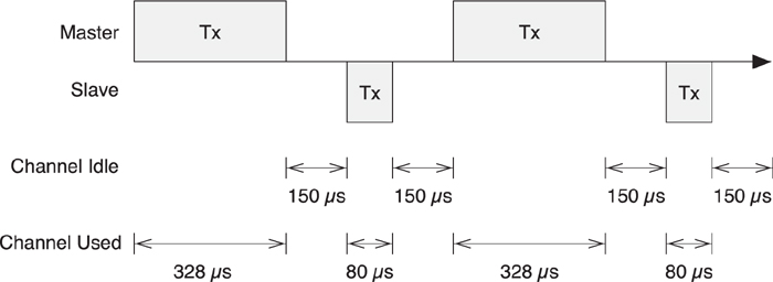
Figure 7–31. Short packets

Therefore, by keeping packets short, there is no need for constant calibration of the radios. This reduces peak power consumption by reducing the quantity and complexity of circuitry that is required to be powered during a packet transmission or reception.

It should also be noted that after transmitting a very long packet, a gap of 150 microseconds is required. This interpacket gap allows the silicon to cool down between packets. Thus, allowing no calibration of frequencies needed between transmitting and receiving or receiving and transmitting packets, further reducing power consumption. This means that when transmitting data in one direction on an encrypted link, the maximum duty cycle is just:

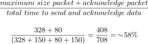
A 58 percent duty cycle is very low for a wireless technology. Bluetooth classic has a duty cycle of 72 percent, whereas very high-speed wireless technologies will have duty cycles in the high 90 percent range. Bluetooth low energy is optimized for small discrete pieces of data being sent, not for the highest possible throughput of data.

7.12.2. High Bit Rate

When transmitting data, a radio requires a large amount of current. Most of this current is consumed by the requirement to run a 2.4GHz oscillator on which the radio signal is modulated. Running very high frequencies in CMOS requires very high currents. CMOS is optimized for gates that don’t change their state all the time because most gates in a digital system do not change state all the time. Any radio running at 2.4GHz built using a bulk CMOS process will therefore use similar current generating this 2.4GHz signal.

Given that it is almost impossible to reduce the power consumption below a certain level because of the oscillator, the efficiency of the modulated signal becomes significant. The quicker you can transmit a given amount of data, the more efficient your radio will be. Bluetooth low energy transmits data at 1,000,000 bits per second.

For example, if a device using another technology can only transmit at a quarter of the rate of Bluetooth low energy, it would take four times as long to transmit a given sequence of bits. Thus, it would take four times as much power to transmit the same amount of data as a Bluetooth low energy system would take. Consequently, high bit rates are a good thing.

It should also be considered that it is possible to go too far on the data rate front. A complex modulation scheme that can transmit, for example, 10 times as many bits per second as Bluetooth low energy would typically take much more power to modulate and demodulate these bits. So, although these bits might take less time to transmit, the extra energy used for modulation means that the power per bit is about the same. However, the current used when receiving nothing, due to clock drift, is significantly higher. Therefore, a simple modulation scheme with low peak-power consumption with high data rates is the most efficient way of sending data. This is the sweet spot that the designers of Bluetooth low energy used.

7.12.3. Low Overhead

Given that every bit counts, the amount of overhead is critically important when considering a radio technology. In Bluetooth low energy, the overhead includes everything that cannot contain application data. This includes the preamble, access address, header, length, the CRC fields, and the optional MIC value.

For an unencrypted packet, the efficiency measured as the size of application data compared with the total packet size required to transmit this data goes from 29 percent to 73 percent, as demonstrated in Table 7–6. The larger the packet, the more efficient the radio is in terms of overhead. For encrypted packets, the efficiency is lower, primarily because of the extra 4 octets of MIC included in each packet. This efficiency is very good, compared with the efficiency of similar proprietary radios. For example, Zigbee has a packet overhead of anywhere from 15 to 31 octets before any encryption overhead. When considering the four-times slower physical bit rate for Zigbee, a short four-octet application data in Zigbee could require up to 10 times more energy than a Bluetooth low energy solution.

Table 7–6. The Overhead for Application Data

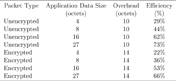
7.12.4. Acknowledgement Scheme

One interesting side effect of the Link Layer acknowledgement scheme is that it does not require that the acknowledgement of a packet be performed, or even delivered, immediately. This is a radical difference between Bluetooth classic and Bluetooth low energy.

In Bluetooth classic, the receiver must acknowledge the packet at the next opportunity it has to transmit. If the acknowledgement is not received immediately, the receiver must signal a negative acknowledgement in the next packet it transmits. This causes the most problems when synchronous links are active and the slave is attempting to send data.

In Bluetooth low energy, every packet sent can acknowledge the last packet transmitted, even if this was transmitted some time ago. This means that devices never have to transmit immediately to send their acknowledgements. The device can choose to wait until it has data to send (or needs to transmit for some other reason, such as timeouts) before acknowledging the last packet. This allows for very fast and efficient acknowledgements that are required when transmitting large quantities of data very quickly.

7.12.5. Single-Channel Connection Events

All communication between a master and a slave occurs in a connection event. A connection event is a packet transmitted by the master, followed by a series of alternating packets sent by the slave and master. In Bluetooth v1.1, every single packet transmitted either as master or slave was transmitted on a different channel. If the master to slave packet was transmitted on one channel, the response would have been sent on a different channel. The problem with this is that even though the slave might have received the master’s transmission perfectly, the next channel that was used for the reply might have interference and, therefore, the acknowledgement for the master’s data packet might not get through.

When it added Adaptive Frequency Hopping, Bluetooth v1.2 made each slave transmission use the same channel as the master’s transmission. In the preceding example, the slave would have replied on the same channel that the master used to transmit its data, and therefore that packet would most likely get through; the assumption is that if a packet is good when data is transmitted from the master to the slave, it will be good when data is transmitted from the slave to the master. This is a good assumption and has improved the actual data rates in heavy interference situations.

Bluetooth low energy has taken this to the logical conclusion. If a channel is good, then why stop using it? If a channel is good, then it should be used for as long as possible. The ultimate invalid conclusion would be to just stop frequency hopping altogether. After all, if the data gets through, then you should just stay on that frequency until it stops working, and then change to another channel at that point.

Unfortunately, at the point when you do need to change frequency, you cannot send any signaling packets to coordinate that change. It also uses a lot of power resynchronizing the single frequency once the channel starts to fail. Given the transient nature of interferers in a location, especially with the bursty nature of much Internet traffic over a Wi-Fi network, this model breaks down very quickly.

This one-channel model also reduces the number of co-located networks because each will naturally drift to a clean frequency. If the number of channels that are clean is small, the number of co-located networks will also be small. A frequency-hopping algorithm distributes network traffic in both time and frequency, allowing for many more simultaneous networks to be active in the same area at the same time. The alternate algorithm—stay on one frequency until it breaks—doesn’t work.

The low-energy approach is to stay on one frequency in a single-connection event, as if you know it works and can send data and acknowledgements, and then move to a new frequency at the next connection event. This means that at any point in time, the frequency to use is fully deterministic. If a particular channel does not work, the two devices will stop using that channel very quickly and resynchronize at the next connection event on a different channel and continue sending data (see Figure 7–32). This means that data can flow with the minimum of latency impacts even where there is lots of interference that is highly unpredictable—a situation that is common in many homes and businesses.

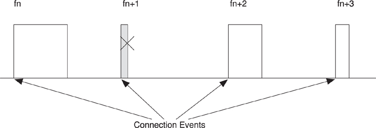
Figure 7–32. Single-channel connection events

7.12.6. Subrating Connection Events

In many situations, the master device has many more resources than the slave device. A computer keyboard has a much smaller battery than the computer, and although the computer might be recharged regularly, the battery in the keyboard is expected to last for years. However, many devices have very small latency requirements. When a user presses a key on a keyboard, that keystroke needs to be delivered to the peer device as quickly as possible. Low latency is a requirement for user interaction. However, the conflicts of low latency and low power have to be resolved.

Low power requires the slave device to only listen for the master device very infrequently. Low latency requires the slave device to be able to transmit as often as possible. Given that the slave cannot talk unless the master speaks to it in a connection event, low latency requires the master to continuously poll the slave to see if it has any data to send. However, if the slave had to listen to each of these connection events, it would not be low power.

The solution is to allow the slave to ignore most connection events from the master, as illustrated in Figure 7–33. The slave would still be able to synchronize and send data at the earliest possible opportunity once it needs to send some data, keeping the latency of data to the connection event interval to that of the master. However, the slave would also be able to ignore a certain number of connection events; this is called the slave latency. The number of connection events that can be missed determines the amount of power that the slave can save. The more connection events that can be missed, the lower power the slave can be.

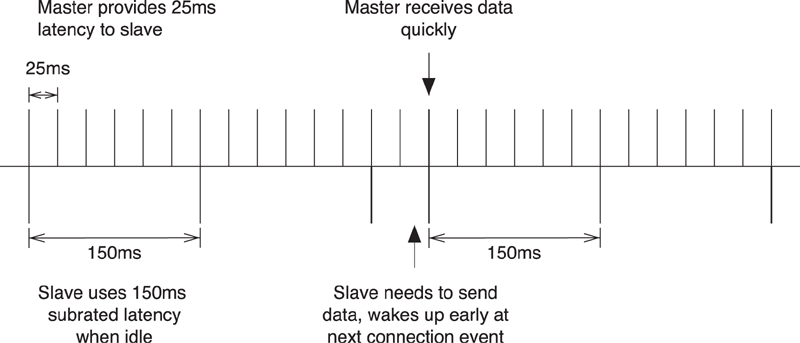
Figure 7–33. Subrated connection events

There is a limit to the slave latency. It is not possible to have a slave latency that is longer than the supervision timeout of the connection. It is also not recommended to have a slave latency that gives fewer than 6 opportunities for the slave to resynchronize to the master. For example, if the supervision timeout is 5 seconds, and the connection event interval was 50 milliseconds, then a slave latency of 4,650 milliseconds would give the slave 6 opportunities to resynchronize at the end of the slave latency. It would also allow the slave to communicate just once every 4.5 seconds, a duty cycle of just 0.0069 percent but still allowing the slave to transmit data to the master in an average time of just 25 milliseconds.

7.12.7. Offline Encryption

Encrypting data is typically considered a very high-power procedure. A device must compute cipher blocks for the payload and message authentication codes as well as compute the authentication code itself. This requires, for a maximum-sized packet, a total of seven iterations of the AES-128 encryption block. If this were required to be performed in real time, the peak current of the packet transmitter and receiver would be significantly higher.

In Bluetooth low energy, the encryption of data and authentication code can be computed in the background. Before a packet is transmitted, the encryption of the data can be performed when the radio is still off. This encryption of data doesn’t depend on the sequence number, the next expected sequence number, or the more data bit. Therefore, the data can be encrypted at any time, from the point it reaches the Link Layer, to just before being transmitted. Also, this data can be retransmitted any number of times, and the encryption and authentication code will not change for each retransmission, even if the next expected sequence number or more data bit changes. This lowers the peak power consumption, and removes the cost of retransmitting encrypted packets.

When receiving encrypted data, the CRC value is computed in real time and is the only value that determines whether the data was received correctly. The encrypted data can be kept in the Link Layer until radio activity stops and there is spare power to decrypt the packet. This decryption of the packet can be done at any time before the packet is delivered to the host. This reduces the peak power for a receiver. Also, if the packet is retransmitted, then upon reception because the sequence number is repeated, it is not necessary to decrypt the packet again. This lowers peak power consumption and removes the cost of re-receiving encrypted packets.