Chapter 19. Understanding OSPF Concepts
This chapter covers the following exam topics:
3.0 IP Connectivity
3.2 Determine how a router makes a forwarding decision by default
3.2.b Administrative distance
3.2.c Routing protocol metric
3.4 Configure and verify single area OSPFv2
3.4.a Neighbor adjacencies
3.4.b Point-to-point
3.4.c Broadcast (DR/BR selection)
3.4.d Router ID
This chapter takes a long look at Open Shortest Path First Version 2 (OSPFv2) concepts. OSPF runs on each router, sending and receiving OSPF messages with neighboring (nearby) routers. These messages give OSPF the means to exchange data about the network and to learn and add IP Version 4 (IPv4) routes to the IPv4 routing table on each router.
Most enterprises over the last 25 years have used either OSPF or the Enhanced Interior Gateway Routing Protocol (EIGRP) for their primary IPv4 routing protocol. For perspective, both OSPF and EIGRP have been part of CCNA throughout most of its 20+ year history. For the CCNA 200-301 exam blueprint, Cisco has included OSPFv2 as the only IPv4 routing protocol. (Note that Cisco does include EIGRP in the CCNP Enterprise certification.)
This chapter breaks the content into three major sections. The first section sets the context about routing protocols in general, defining interior and exterior routing protocols and basic routing protocol features and terms. The second major section presents the nuts and bolts of how OSPFv2 works, using OSPF neighbor relationships, database exchange, and then route calculation. The third section wraps up the discussion by looking at OSPF areas and LSAs.
“Do I Know This Already?” Quiz
Take the quiz (either here or use the PTP software) if you want to use the score to help you decide how much time to spend on this chapter. The letter answers are listed at the bottom of the page following the quiz. Appendix C, found both at the end of the book as well as on the companion website, includes both the answers and explanations. You can also find both answers and explanations in the PTP testing software.
Table 19-1 “Do I Know This Already?” Foundation Topics Section-to-Question Mapping
Foundation Topics Section |
Questions |
|---|---|
Comparing Dynamic Routing Protocol Features |
1–3 |
OSPF Concepts and Operation |
4, 5 |
OSPF Areas and LSAs |
6 |
1. Which of the following routing protocols is considered to use link-state logic?
a. RIPv1
b. RIPv2
c. EIGRP
d. OSPF
2. Which of the following routing protocols use a metric that is, by default, at least partially affected by link bandwidth? (Choose two answers.)
a. RIPv1
b. RIPv2
c. EIGRP
d. OSPF
3. Which of the following interior routing protocols support VLSM? (Choose three answers.)
a. RIPv1
b. RIPv2
c. EIGRP
d. OSPF
4. Two routers using OSPFv2 have become neighbors and exchanged all LSAs. As a result, Router R1 now lists some OSPF-learned routes in its routing table. Which of the following best describes how R1 uses those recently learned LSAs to choose which IP routes to add to its IP routing table?
a. Each LSA lists a route to be copied to the routing table.
b. Some LSAs list a route that can be copied to the routing table.
c. Run some SPF math against the LSAs to calculate the routes.
d. R1 does not use the LSAs at all when choosing what routes to add.
5. Which of the following OSPF neighbor states is expected when the exchange of topology information is complete between two OSPF neighbors?
a. 2-way
b. Full
c. Up/up
d. Final
6. A company has a small/medium-sized network with 15 routers and 40 subnets and uses OSPFv2. Which of the following is considered an advantage of using a single-area design as opposed to a multiarea design?
a. It reduces the processing overhead on most routers.
b. Status changes to one link may not require SPF to run on all other routers.
c. It allows for simpler planning and operations.
d. It allows for route summarization, reducing the size of IP routing tables.
Answers to the “Do I Know This Already?” quiz:
1 D
2 C, D
3 B, C, D
4 C
5 B
6 C
Foundation Topics
Comparing Dynamic Routing Protocol Features
Routers add IP routes to their routing tables using three methods: connected routes, static routes, and routes learned by using dynamic routing protocols. Before we get too far into the discussion, however, it is important to define a few related terms and clear up any misconceptions about the terms routing protocol, routed protocol, and routable protocol. The concepts behind these terms are not that difficult, but because the terms are so similar, and because many documents pay poor attention to when each of these terms is used, they can be a bit confusing. These terms are generally defined as follows:
Routing protocol: A set of messages, rules, and algorithms used by routers for the overall purpose of learning routes. This process includes the exchange and analysis of routing information. Each router chooses the best route to each subnet (path selection) and finally places those best routes in its IP routing table. Examples include RIP, EIGRP, OSPF, and BGP.
Routed protocol and routable protocol: Both terms refer to a protocol that defines a packet structure and logical addressing, allowing routers to forward or route the packets. Routers forward packets defined by routed and routable protocols. Examples include IP Version 4 (IPv4) and IP Version 6 (IPv6).
Note
The term path selection sometimes refers to part of the job of a routing protocol, in which the routing protocol chooses the best route.
Even though routing protocols (such as OSPF) are different from routed protocols (such as IP), they do work together very closely. The routing process forwards IP packets, but if a router does not have any routes in its IP routing table that match a packet’s destination address, the router discards the packet. Routers need routing protocols so that the routers can learn all the possible routes and add them to the routing table so that the routing process can forward (route) routable protocols such as IP.
Routing Protocol Functions
Cisco IOS software supports several IP routing protocols, performing the same general functions:
Learn routing information about IP subnets from neighboring routers.
Advertise routing information about IP subnets to neighboring routers.
If more than one possible route exists to reach one subnet, pick the best route based on a metric.
If the network topology changes—for example, a link fails—react by advertising that some routes have failed and pick a new currently best route. (This process is called convergence.)
Note
A neighboring router connects to the same link as another router, such as the same WAN link or the same Ethernet LAN.
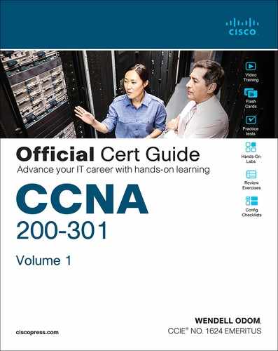
Figure 19-1 shows an example of three of the four functions in the list. Router R1, in the lower left of the figure, must make a decision about the best route to reach the subnet connected off router R2, on the bottom right of the figure. Following the steps in the figure:
Step 1. R2 advertises a route to the lower right subnet—172.16.3.0/24—to both router R1 and R3.
Step 2. After R3 learns about the route to 172.16.3.0/24 from R2, R3 advertises that route to R1.
Step 3. R1 must make a decision about the two routes it learned about for reaching subnet 172.16.3.0/24—one with metric 1 from R2 and one with metric 2 from R3. R1 chooses the lower metric route through R2 (function 3).
The other routing protocol function, convergence, occurs when the topology changes—that is, when either a router or link fails or comes back up again. When something changes, the best routes available in the network can change. Convergence simply refers to the process by which all the routers collectively realize something has changed, advertise the information about the changes to all the other routers, and all the routers then choose the currently best routes for each subnet. The ability to converge quickly, without causing loops, is one of the most important considerations when choosing which IP routing protocol to use.
In Figure 19-1, convergence might occur if the link between R1 and R2 failed. In that case, R1 should stop using its old route for subnet 172.16.3.0/24 (directly through R2) and begin sending packets to R3.
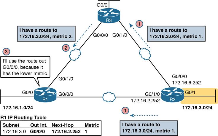
Figure 19-1 Three of the Four Basic Functions of Routing Protocols
Interior and Exterior Routing Protocols
IP routing protocols fall into one of two major categories: interior gateway protocols (IGP) or exterior gateway protocols (EGP). The definitions of each are as follows:

IGP: A routing protocol that was designed and intended for use inside a single autonomous system (AS)
EGP: A routing protocol that was designed and intended for use between different autonomous systems
Note
The terms IGP and EGP include the word gateway because routers used to be called gateways.
These definitions use another new term: autonomous system (AS). An AS is a network under the administrative control of a single organization. For example, a network created and paid for by a single company is probably a single AS, and a network created by a single school system is probably a single AS. Other examples include large divisions of a state or national government, where different government agencies might be able to build their own networks. Each ISP is also typically a single different AS.
Some routing protocols work best inside a single AS by design, so these routing protocols are called IGPs. Conversely, routing protocols designed to exchange routes between routers in different autonomous systems are called EGPs. Today, Border Gateway Protocol (BGP) is the only EGP used.
Each AS can be assigned a number called (unsurprisingly) an AS number (ASN). Like public IP addresses, the Internet Assigned Numbers Authority (IANA, www.iana.org) controls the worldwide rights to assigning ASNs. It delegates that authority to other organizations around the world, typically to the same organizations that assign public IP addresses. For example, in North America, the American Registry for Internet Numbers (ARIN, www.arin.net) assigns public IP address ranges and ASNs.
Figure 19-2 shows a small view of the worldwide Internet. The figure shows two enterprises and three ISPs using IGPs (OSPF and EIGRP) inside their own networks and with BGP being used between the ASNs.
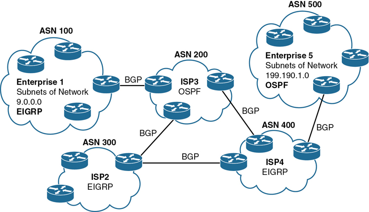
Figure 19-2 Comparing Locations for Using IGPs and EGPs
Comparing IGPs
Organizations have several options when choosing an IGP for their enterprise network, but most companies today use either OSPF or EIGRP. This book discusses OSPFv2, with the CCNP Enterprise certification adding EIGRP. Before getting into detail on these two protocols, the next section first discusses some of the main goals of every IGP, comparing OSPF, EIGRP, plus a few other IPv4 routing protocols.
IGP Routing Protocol Algorithms
A routing protocol’s underlying algorithm determines how the routing protocol does its job. The term routing protocol algorithm simply refers to the logic and processes used by different routing protocols to solve the problem of learning all routes, choosing the best route to each subnet, and converging in reaction to changes in the internetwork. Three main branches of routing protocol algorithms exist for IGP routing protocols:
Distance vector (sometimes called Bellman-Ford after its creators)
Advanced distance vector (sometimes called “balanced hybrid”)
Link-state
Historically speaking, distance vector protocols were invented first, mainly in the early 1980s. Routing Information Protocol (RIP) was the first popularly used IP distance vector protocol, with the Cisco-proprietary Interior Gateway Routing Protocol (IGRP) being introduced a little later.
By the early 1990s, distance vector protocols’ somewhat slow convergence and potential for routing loops drove the development of new alternative routing protocols that used new algorithms. Link-state protocols—in particular, Open Shortest Path First (OSPF) and Integrated Intermediate System to Intermediate System (IS-IS)—solved the main issues. They also came with a price: they required extra CPU and memory on routers, with more planning required from the network engineers.
Note
All references to OSPF in this chapter refer to OSPFv2 unless otherwise stated.
Around the same time as the introduction of OSPF, Cisco created a proprietary routing protocol called Enhanced Interior Gateway Routing Protocol (EIGRP), which used some features of the earlier IGRP protocol. EIGRP solved the same problems as did link-state routing protocols, but EIGRP required less planning when implementing the network. As time went on, EIGRP was classified as a unique type of routing protocol. However, it used more distance vector features than link-state, so it is more commonly classified as an advanced distance vector protocol.
Metrics
Routing protocols choose the best route to reach a subnet by choosing the route with the lowest metric. For example, RIP uses a counter of the number of routers (hops) between a router and the destination subnet, as shown in the example of Figure 19-1. OSPF totals the cost associated with each interface in the end-to-end route, with the cost based on link bandwidth. Table 19-2 lists the most common IP routing protocols and some details about the metric in each case.
Table 19-2 IP IGP Metrics
IGP |
Metric |
Description |
|---|---|---|
RIPv2 |
Hop count |
The number of routers (hops) between a router and the destination subnet |
OSPF |
Cost |
The sum of all interface cost settings for all links in a route, with the cost defaulting to be based on interface bandwidth |
EIGRP |
Calculation based on bandwidth and delay |
Calculated based on the route’s slowest link and the cumulative delay associated with each interface in the route |
A brief comparison of the metric used by the older RIP versus the metric used by OSPF shows some insight into why OSPF and EIGRP surpassed RIP. Figure 19-3 shows an example in which Router B has two possible routes to subnet 10.1.1.0 on the left side of the network: a shorter route over a very slow serial link at 1544 Kbps, or a longer route over two Gigabit Ethernet WAN links.
Figure 19-3 RIP and OSPF Metrics Compared
The left side of the figure shows the results of RIP in this network. Using hop count, Router B learns of a one-hop route directly to Router A through B’s S0/0/1 interface. B also learns of a two-hop route through Router C, through B’s G0/0 interface. Router B chooses the lower hop count route, which happens to go over the slow-speed serial link.
The right side of the figure shows the better choice made by OSPF based on its better metric. To cause OSPF to make the right choice, the engineer could use default settings based on the correct interface bandwidth to match the actual link speeds, thereby allowing OSPF to choose the faster route. (The bandwidth interface subcommand does not change the actual physical speed of the interface. It just tells IOS what speed to assume the interface is using.)
Other IGP Comparisons
Routing protocols can be compared based on many features, some of which matter to the current CCNA exam, whereas some do not. Table 19-3 introduces a few more points and lists the comparison points mentioned in this book for easier study, with a few supporting comments following the table.
Table 19-3 Interior IP Routing Protocols Compared
Feature |
RIPv2 |
EIGRP |
OSPF |
|---|---|---|---|
Classless/sends mask in updates/supports VLSM |
Yes |
Yes |
Yes |
Algorithm (DV, advanced DV, LS) |
DV |
Advanced DV |
LS |
Supports manual summarization |
Yes |
Yes |
Yes |
Cisco-proprietary |
No |
Yes1 |
No |
Routing updates are sent to a multicast IP address |
Yes |
Yes |
Yes |
Convergence |
Slow |
Fast |
Fast |
1 Although Cisco created EIGRP and has kept it as a proprietary protocol for many years, Cisco chose to publish EIGRP as an informational RFC in 2013. This allows other vendors to implement EIGRP, while Cisco retains the rights to the protocol.
Regarding the top row of the table, routing protocols can be considered to be a classless routing protocol or a classful routing protocol. Classless routing protocols support variable-length subnet masks (VLSM) as well as manual route summarization by sending routing protocol messages that include the subnet masks in the message. The older RIPv1 and IGRP routing protocols—both classful routing protocols—do not.
Also, note that the older routing protocols (RIPv1, IGRP) sent routing protocol messages as IP broadcast addresses, while the newer routing protocols in the table all use IP multicast destination addresses. The use of multicasts makes the protocol more efficient and causes less overhead and fewer issues with the devices in the subnet that are not running the routing protocol.
Administrative Distance
Many companies and organizations use a single routing protocol. However, in some cases, a company needs to use multiple routing protocols. For example, if two companies connect their networks so that they can exchange information, they need to exchange some routing information. If one company uses OSPF and the other uses EIGRP on at least one router, both OSPF and EIGRP must be used. Then that router can take routes learned by OSPF and advertise them into EIGRP, and vice versa, through a process called route redistribution.
Depending on the network topology, the two routing protocols might learn routes to the same subnets. When a single routing protocol learns multiple routes to the same subnet, the metric tells it which route is best. However, when two different routing protocols learn routes to the same subnet, because each routing protocol’s metric is based on different information, IOS cannot compare the metrics. For example, OSPF might learn a route to subnet 10.1.1.0 with metric 101, and EIGRP might learn a route to 10.1.1.0 with metric 2,195,416, but the EIGRP-learned route might be the better route—or it might not. There is simply no basis for comparison between the two metrics.
When IOS must choose between routes learned using different routing protocols, IOS uses a concept called administrative distance. Administrative distance is a number that denotes how believable an entire routing protocol is on a single router. The lower the number, the better, or more believable, the routing protocol. For example, RIP has a default administrative distance of 120, OSPF uses a default of 110, and EIGRP defaults to 90. When using OSPF and EIGRP, the router will believe the EIGRP route instead of the OSPF route (at least by default). The administrative distance values are configured on a single router and are not exchanged with other routers. Table 19-4 lists the various sources of routing information, along with the default administrative distances.
Table 19-4 Default Administrative Distances
Route Type |
Administrative Distance |
|---|---|
Connected |
0 |
Static |
1 |
BGP (external routes [eBGP]) |
20 |
EIGRP (internal routes) |
90 |
IGRP |
100 |
OSPF |
110 |
IS-IS |
115 |
RIP |
120 |
EIGRP (external routes) |
170 |
BGP (internal routes [iBGP]) |
200 |
DHCP default route |
254 |
Unusable |
255 |
Note
The show ip route command lists each route’s administrative distance as the first of the two numbers inside the brackets. The second number in brackets is the metric.
The table shows the default administrative distance values, but IOS can be configured to change the administrative distance of a particular routing protocol, a particular route, or even a static route. For example, the command ip route 10.1.3.0 255.255.255.0 10.1.130.253 defines a static route with a default administrative distance of 1, but the command ip route 10.1.3.0 255.255.255.0 10.1.130.253 210 defines the same static route with an administrative distance of 210. So, you can actually create a static route that is only used when the routing protocol does not find a route, just by giving the static route a higher administrative distance.
OSPF Concepts and Operation
Routing protocols basically exchange information so routers can learn routes. The routers learn information about subnets, routes to those subnets, and metric information about how good each route is compared to others. The routing protocol can then choose the currently best route to each subnet, building the IP routing table.
Link-state protocols like OSPF take a little different approach to the particulars of what information they exchange and what the routers do with that information once learned. This next (second) major section narrows the focus to only link-state protocols, specifically OSPFv2.
This section begins with an overview of what OSPF does by exchanging data about the network in data structures called link-state advertisements (LSA). Then the discussion backs up a bit to provide more details about each of three fundamental parts of how OSPF operates: how OSPF routers use neighbor relationships, how routers exchange LSAs with neighbors, and then how routers calculate the best routes once they learn all the LSAs.
OSPF Overview
Link-state protocols build IP routes with a couple of major steps. First, the routers together build a lot of information about the network: routers, links, IP addresses, status information, and so on. Then the routers flood the information, so all routers know the same information. At that point, each router can calculate routes to all subnets, but from each router’s own perspective.
Topology Information and LSAs
Routers using link-state routing protocols need to collectively advertise practically every detail about the internetwork to all the other routers. At the end of the process of flooding the information to all routers, every router in the internetwork has the exact same information about the internetwork. Flooding a lot of detailed information to every router sounds like a lot of work, and relative to distance vector routing protocols, it is.
Open Shortest Path First (OSPF), the most popular link-state IP routing protocol, organizes topology information using LSAs and the link-state database (LSDB). Figure 19-4 represents the ideas. Each LSA is a data structure with some specific information about the network topology; the LSDB is simply the collection of all the LSAs known to a router.
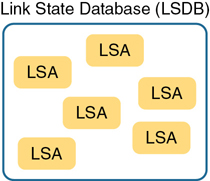
Figure 19-4 LSA and LSDB Relationship
Figure 19-5 shows the general idea of the flooding process, with R8 creating and flooding its router LSA. The router LSA for Router R8 describes the router itself, including the existence of subnet 172.16.3.0/24, as seen on the right side of the figure. (Note that Figure 19-5 actually shows only a subset of the information in R8’s router LSA.)
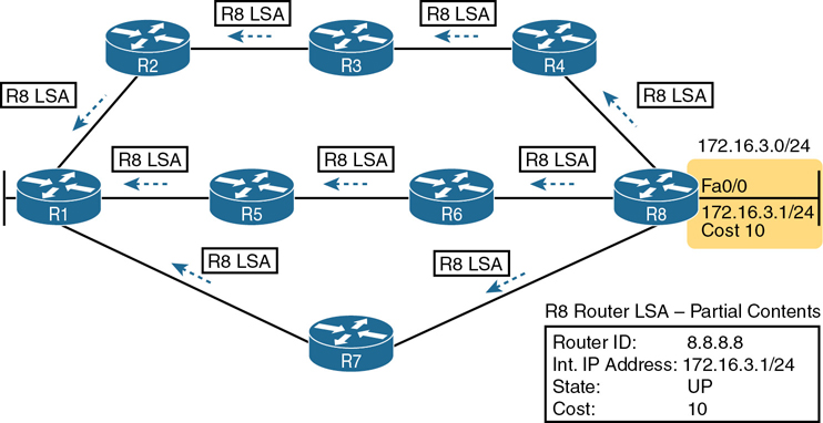
Figure 19-5 Flooding LSAs Using a Link-State Routing Protocol
Figure 19-5 shows the rather basic flooding process, with R8 sending the original LSA for itself, and the other routers flooding the LSA by forwarding it until every router has a copy. The flooding process causes every router to learn the contents of the LSA while preventing the LSA from being flooded around in circles. Basically, before sending an LSA to yet another neighbor, routers communicate, asking “Do you already have this LSA?,” and then sending the LSA to the next neighbor only if the neighbor has not yet learned about the LSA.
Once flooded, routers do occasionally reflood each LSA. Routers reflood an LSA when some information changes (for example, when a link goes up or comes down). They also reflood each LSA based on each LSA’s separate aging timer (default 30 minutes).
Applying Dijkstra SPF Math to Find the Best Routes
The link-state flooding process results in every router having an identical copy of the LSDB in memory, but the flooding process alone does not cause a router to learn what routes to add to the IP routing table. Although incredibly detailed and useful, the information in the LSDB does not explicitly state each router’s best route to reach a destination.
To build routes, link-state routers have to do some math. Thankfully, you and I do not have to know the math! However, all link-state protocols use a type of math algorithm, called the Dijkstra Shortest Path First (SPF) algorithm, to process the LSDB. That algorithm analyzes (with math) the LSDB and builds the routes that the local router should add to the IP routing table—routes that list a subnet number and mask, an outgoing interface, and a next-hop router IP address.
Now that you have the big ideas down, the next several topics walk through the three main phases of how OSPF routers accomplish the work of exchanging LSAs and calculating routes. Those three phases are
Becoming neighbors: A relationship between two routers that connect to the same data link, created so that the neighboring routers have a means to exchange their LSDBs.
Exchanging databases: The process of sending LSAs to neighbors so that all routers learn the same LSAs.
Adding the best routes: The process of each router independently running SPF, on their local copy of the LSDB, calculating the best routes, and adding those to the IPv4 routing table.
Becoming OSPF Neighbors
Of everything you learn about OSPF in this chapter, OSPF neighbor concepts have the most to do with how you will configure and troubleshoot OSPF in Cisco routers. You configure OSPF to cause routers to run OSPF and become neighbors with other routers. Once that happens, OSPF does the rest of the work to exchange LSAs and calculate routers in the background, with no additional configuration required. This section discusses the fundamental concepts of OSPF neighbors.
The Basics of OSPF Neighbors
OSPF neighbors are routers that both use OSPF and both sit on the same data link. Two routers can become OSPF neighbors if connected to the same VLAN, or same serial link, or same Ethernet WAN link.
Two routers need to do more than simply exist on the same link to become OSPF neighbors; they must send OSPF messages and agree to become OSPF neighbors. To do so, the routers send OSPF Hello messages, introducing themselves to the potential neighbor. Assuming the two potential neighbors have compatible OSPF parameters, the two form an OSPF neighbor relationship, and would be displayed in the output of the show ip ospf neighbor command.
The OSPF neighbor relationship also lets OSPF know when a neighbor might not be a good option for routing packets right now. Imagine R1 and R2 form a neighbor relationship, learn LSAs, and calculate routes that send packets through the other router. Months later, R1 notices that the neighbor relationship with R2 fails. That failed neighbor connection to R2 makes R1 react: R1 refloods LSAs impacted by the failed link, and R1 runs SPF to recalculate its own routes.
Finally, the OSPF neighbor model allows new routers to be dynamically discovered. That means new routers can be added to a network without requiring every router to be reconfigured. Instead, OSPF routers listen for OSPF Hello messages from new routers and react to those messages, attempting to become neighbors and exchange LSDBs.
Meeting Neighbors and Learning Their Router ID
The OSPF Hello process, by which new neighbor relationships are formed, works somewhat like when you move to a new house and meet your various neighbors. When you see each other outside, you might walk over, say hello, and learn each other’s name. After talking a bit, you form a first impression, particularly as to whether you think you’ll enjoy chatting with this neighbor occasionally, or whether you can just wave and not take the time to talk the next time you see him outside.
Similarly, with OSPF, the process starts with messages called OSPF Hello messages. The Hellos in turn list each router’s router ID (RID), which serves as each router’s unique name or identifier for OSPF. Finally, OSPF does several checks of the information in the Hello messages to ensure that the two routers should become neighbors.
OSPF RIDs are 32-bit numbers. As a result, most command output lists these as dotted-decimal numbers (DDN). By default, IOS chooses one of the router’s interface IPv4 addresses to use as its OSPF RID. However, the OSPF RID can be directly configured, as covered in the section “Configuring the OSPF Router ID” in Chapter 20, “Implementing OSPF.”
As soon as a router has chosen its OSPF RID and some interfaces come up, the router is ready to meet its OSPF neighbors. OSPF routers can become neighbors if they are connected to the same subnet. To discover other OSPF-speaking routers, a router sends multicast OSPF Hello packets to each interface and hopes to receive OSPF Hello packets from other routers connected to those interfaces. Figure 19-6 outlines the basic concept.
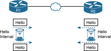
Figure 19-6 OSPF Hello Packets
Routers R1 and R2 both send Hello messages onto the link. They continue to send Hellos at a regular interval based on their Hello timer settings. The Hello messages themselves have the following features:
The Hello message follows the IP packet header, with IP protocol type 89.
Hello packets are sent to multicast IP address 224.0.0.5, a multicast IP address intended for all OSPF-speaking routers.
OSPF routers listen for packets sent to IP multicast address 224.0.0.5, in part hoping to receive Hello packets and learn about new neighbors.
Taking a closer look, Figure 19-7 shows several of the neighbor states used by the early formation of an OSPF neighbor relationship. The figure shows the Hello messages in the center and the resulting neighbor states on the left and right edges of the figure. Each router keeps an OSPF state variable for how it views the neighbor.
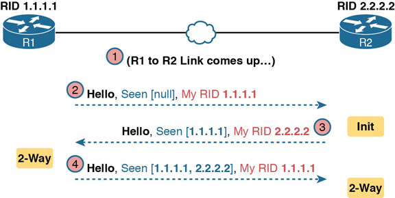
Figure 19-7 Early Neighbor States
Following the steps in the figure, the scenario begins with the link down, so the routers have no knowledge of each other as OSPF neighbors. As a result, they have no state (status) information about each other as neighbors, and they would not list each other in the output of the show ip ospf neighbor command. At Step 2, R1 sends the first Hello, so R2 learns of the existence of R1 as an OSPF router. At that point, R2 lists R1 as a neighbor, with an interim beginning state of init.
The process continues at Step 3, with R2 sending back a Hello. This message tells R1 that R2 exists, and it allows R1 to move through the init state and quickly to a 2-way state. At Step 4, R2 receives the next Hello from R1, and R2 can also move to a 2-way state.
The 2-way state is a particularly important OSPF state. At that point, the following major facts are true:
The router received a Hello from the neighbor, with that router’s own RID listed as being seen by the neighbor.
The router has checked all the parameters in the Hello received from the neighbor, with no problems. The router is willing to become an OSPF neighbor.
If both routers reach a 2-way state with each other, it means that both routers meet all OSPF configuration requirements to become neighbors. Effectively, at that point, they are neighbors and ready to exchange their LSDB with each other.
Exchanging the LSDB Between Neighbors
One purpose of forming OSPF neighbor relationships is to allow the two neighbors to exchange their databases. This next topic works through some of the details of OSPF database exchange.
Fully Exchanging LSAs with Neighbors
The OSPF neighbor state 2-way means that the router is available to exchange its LSDB with the neighbor. In other words, it is ready to begin a 2-way exchange of the LSDB. So, once two routers on a link reach the 2-way state, they can immediately move on to the process of database exchange.
The database exchange process can be quite involved, with several OSPF messages and several interim neighbor states. This chapter is more concerned with a few of the messages and the final state when database exchange has completed: the full state.
After two routers decide to exchange databases, they do not simply send the contents of the entire database. First, they tell each other a list of LSAs in their respective databases—not all the details of the LSAs, just a list. (Think of these lists as checklists.) Then each router can check which LSAs it already has and then ask the other router for only the LSAs that are not known yet.
For instance, R1 might send R2 a checklist that lists 10 LSAs (using an OSPF Database Description, or DD, packet). R2 then checks its LSDB and finds six of those 10 LSAs. So, R2 asks R1 (using a Link-State Request packet) to send the four additional LSAs.
Thankfully, most OSPFv2 work does not require detailed knowledge of these specific protocol steps. However, a few of the terms are used quite a bit and should be remembered. In particular, the OSPF messages that actually send the LSAs between neighbors are called Link-State Update (LSU) packets. That is, the LSU packet holds data structures called link-state advertisements (LSA). The LSAs are not packets, but rather data structures that sit inside the LSDB and describe the topology.
Figure 19-8 pulls some of these terms and processes together, with a general example. The story picks up the example shown in Figure 19-7, with Figure 19-8 showing an example of the database exchange process between Routers R1 and R2. The center shows the protocol messages, and the outer items show the neighbor states at different points in the process. Focus on two items in particular:
The routers exchange the LSAs inside LSU packets.
When finished, the routers reach a full state, meaning they have fully exchanged the contents of their LSDBs.
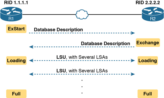
Figure 19-8 Database Exchange Example, Ending in a Full State
Maintaining Neighbors and the LSDB
Once two neighbors reach a full state, they have done all the initial work to exchange OSPF information between them. However, neighbors still have to do some small ongoing tasks to maintain the neighbor relationship.
First, routers monitor each neighbor relationship using Hello messages and two related timers: the Hello Interval and the Dead Interval. Routers send Hellos every Hello Interval to each neighbor. Each router expects to receive a Hello from each neighbor based on the Hello Interval, so if a neighbor is silent for the length of the Dead Interval (by default, four times as long as the Hello Interval), the loss of Hellos means that the neighbor has failed.
Next, routers must react when the topology changes as well, and neighbors play a key role in that process. When something changes, one or more routers change one or more LSAs. Then the routers must flood the changed LSAs to each neighbor so that the neighbor can change its LSDB.
For example, imagine a LAN switch loses power, so a router’s G0/0 interface fails from up/up to down/down. That router updates an LSA that shows the router’s G0/0 as being down. That router then sends the LSA to its neighbors, and that neighbor in turn sends it to its neighbors, until all routers again have an identical copy of the LSDB. Each router’s LSDB now reflects the fact that the original router’s G0/0 interface failed, so each router will then use SPF to recalculate any routes affected by the failed interface.
A third maintenance task done by neighbors is to reflood each LSA occasionally, even when the network is completely stable. By default, each router that creates an LSA also has the responsibility to reflood the LSA every 30 minutes (the default), even if no changes occur. (Note that each LSA has a separate timer, based on when the LSA was created, so there is no single big event where the network is overloaded with flooding LSAs.)
The following list summarizes these three maintenance tasks for easier review:
Maintain neighbor state by sending Hello messages based on the Hello Interval and listening for Hellos before the Dead Interval expires
Flood any changed LSAs to each neighbor
Reflood unchanged LSAs as their lifetime expires (default 30 minutes)
Using Designated Routers on Ethernet Links
OSPF behaves differently on some types of interfaces based on a per-interface setting called the OSPF network type. On Ethernet links, OSPF defaults to use a network type of broadcast, which causes OSPF to elect one of the routers on the same subnet to act as the designated router (DR). The DR plays a key role in how the database exchange process works, with different rules than with point-to-point links.
To see how, consider the example that begins with Figure 19-9. The figure shows five OSPFv2 routers on the same Ethernet VLAN. These five OSPF routers elect one router to act as the DR and one router to be a backup DR (BDR). The figure shows A and B as DR and BDR, for no other reason than the Ethernet must have one of each.
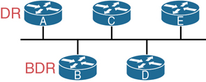
Figure 19-9 Routers A and B Elected as DR and BDR
The database exchange process on an Ethernet link does not happen between every pair of routers on the same VLAN/subnet. Instead, it happens between the DR and each of the other routers, with the DR making sure that all the other routers get a copy of each LSA. In other words, the database exchange happens over the flows shown in Figure 19-10.
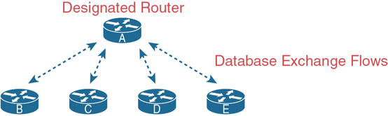
Figure 19-10 Database Exchange to and from the DR on an Ethernet
OSPF uses the BDR concept because the DR is so important to the database exchange process. The BDR watches the status of the DR and takes over for the DR if it fails. (When the DR fails, the BDR takes over, and then a new BDR is elected.)
The use of a DR/BDR, along with the use of multicast IP addresses, makes the exchange of OSPF LSDBs more efficient on networks that allow more than two routers on the same link. The DR can send a packet to all OSPF routers in the subnet by using multicast IP address 224.0.0.5. IANA reserves this address as the “All SPF Routers” multicast address just for this purpose. For instance, in Figure 19-10, the DR can send one set of messages to all the OSPF routers rather than sending one message to each router.
Similarly, any OSPF router needing to send a message to the DR and also to the BDR (so it remains ready to take over for the DR) can send those messages to the “All SPF DRs” multicast address 224.0.0.6. So, instead of having to send one set of messages to the DR and another set to the BDR, an OSPF router can send one set of messages, making the exchange more efficient.
At this point, you might be getting a little tired of some of the theory, but finally, the theory actually shows something that you may see in show commands on a router. Because the DR and BDR both do full database exchange with all the other OSPF routers in the LAN, they reach a full state with all neighbors. However, routers that are neither a DR nor a BDR—called DROthers by OSPF—never reach a full state because they do not exchange LSDBs directly with each other. As a result, the show ip ospf neighbor command on these DROther routers lists some neighbors in a 2-way state, remaining in that state under normal operation.
For instance, with OSPF working normally on the Ethernet LAN in Figure 19-10, a show ip ospf neighbor command on router C (which is a DROther router) would show the following:
Two neighbors (A and B, the DR and BDR, respectively) with a full state (called fully adjacent neighbors)
Two neighbors (D and E, which are DROthers) with a 2-way state (called neighbors)
OSPF requires some terms to describe all neighbors versus the subset of all neighbors that reach the full state. First, all OSPF routers on the same link that reach the 2-way state—that is, they send Hello messages and the parameters match—are called neighbors. The subset of neighbors for which the neighbor relationship continues on and reaches the full state are called adjacent neighbors. Additionally, OSPFv2 RFC 2328 emphasizes the connection between the full state and the term adjacent neighbor by using the synonyms of fully adjacent and fully adjacent neighbor. Finally, while the terms so far refer to the neighbor, two other terms refer to the relationship: neighbor relationship refers to any OSPF neighbor relationship, while the term adjacency refers to neighbor relationships that reach a full state. Table 19-5 details the terms.
Table 19-5 Stable OSPF Neighbor States and Their Meanings
Neighbor State |
Term for Neighbor |
Term for Relationship |
|---|---|---|
2-way |
Neighbor |
Neighbor Relationship |
Full |
Adjacent Neighbor Fully Adjacent Neighbor |
Adjacency |
Calculating the Best Routes with SPF
OSPF LSAs contain useful information, but they do not contain the specific information that a router needs to add to its IPv4 routing table. In other words, a router cannot just copy information from the LSDB into a route in the IPv4 routing table. The LSAs individually are more like pieces of a jigsaw puzzle. So, to know what routes to add to the routing table, each router must do some SPF math to choose the best routes from that router’s perspective. The router then adds each route to its routing table: a route with a subnet number and mask, an outgoing interface, and a next-hop router IP address.
Although engineers do not need to know the details of how SPF does the math, they do need to know how to predict which routes SPF will choose as the best route. The SPF algorithm calculates all the routes for a subnet—that is, all possible routes from the router to the destination subnet. If more than one route exists, the router compares the metrics, picking the best (lowest) metric route to add to the routing table. Although the SPF math can be complex, engineers with a network diagram, router status information, and simple addition can calculate the metric for each route, predicting what SPF will choose.
Once SPF has identified a route, OSPF calculates the metric for a route as follows:
The sum of the OSPF interface costs for all outgoing interfaces in the route.
Figure 19-11 shows an example with three possible routes from R1 to Subnet X (172.16.3.0/24) at the bottom of the figure.
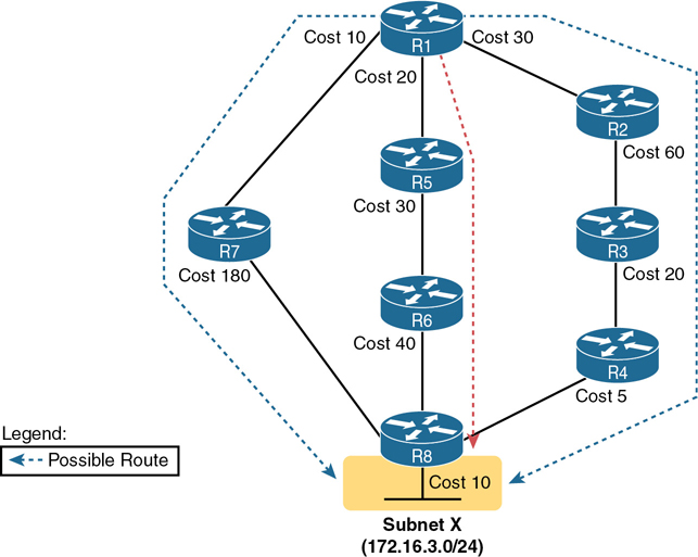
Figure 19-11 SPF Tree to Find R1’s Route to 172.16.3.0/24
Note
OSPF considers the costs of the outgoing interfaces (only) in each route. It does not add the cost for incoming interfaces in the route.
Table 19-6 lists the three routes shown in Figure 19-11, with their cumulative costs, showing that R1’s best route to 172.16.3.0/24 starts by going through R5.
Table 19-6 Comparing R1’s Three Alternatives for the Route to 172.16.3.0/24
Route |
Location in Figure 19-11 |
Cumulative Cost |
|---|---|---|
R1–R7–R8 |
Left |
10 + 180 + 10 = 200 |
R1–R5–R6–R8 |
Middle |
20 + 30 + 40 + 10 = 100 |
R1–R2–R3–R4–R8 |
Right |
30 + 60 + 20 + 5 + 10 = 125 |
As a result of the SPF algorithm’s analysis of the LSDB, R1 adds a route to subnet 172.16.3.0/24 to its routing table, with the next-hop router of R5.
In real OSPF networks, an engineer can do the same process by knowing the OSPF cost for each interface. Armed with a network diagram, the engineer can examine all routes, add the costs, and predict the metric for each route.
OSPF Areas and LSAs
OSPF can be used in some networks with very little thought about design issues. You just turn on OSPF in all the routers, put all interfaces into the same area (usually area 0), and it works! Figure 19-12 shows one such network example, with 11 routers and all interfaces in area 0.

Figure 19-12 Single-Area OSPF
Larger OSPFv2 networks suffer with a single-area design. For instance, now imagine an enterprise network with 900 routers, rather than only 11, and several thousand subnets. As it turns out, the CPU time to run the SPF algorithm on all that topology data just takes time. As a result, OSPFv2 convergence time—the time required to react to changes in the network—can be slow. The routers might run low on RAM as well. Additional problems with a single area design include the following:
A larger topology database requires more memory on each router.
The SPF algorithm requires processing power that grows exponentially compared to the size of the topology database.
A single interface status change anywhere in the internetwork (up to down, or down to up) forces every router to run SPF again!
The solution is to take the one large LSDB and break it into several smaller LSDBs by using OSPF areas. With areas, each link is placed into one area. SPF does its complicated math on the topology inside the area, and that area’s topology only. For instance, an internetwork with 1000 routers and 2000 subnets, broken in 100 areas, would average 10 routers and 20 subnets per area. The SPF calculation on a router would have to only process topology about 10 routers and 20 links, rather than 1000 routers and 2000 links.
So, how large does a network have to be before OSPF needs to use areas? Well, there is no set answer because the behavior of the SPF process depends largely on CPU processing speed, the amount of RAM, the size of the LSDB, and so on. Generally, networks larger than a few dozen routers benefit from areas, and some documents over the years have listed 50 routers as the dividing line at which a network really should use multiple OSPF areas.
The next few pages look at how OSPF area design works, with more reasons as to why areas help make larger OSPF networks work better.
OSPF Areas
OSPF area design follows a couple of basic rules. To apply the rules, start with a clean drawing of the internetwork, with routers, and all interfaces. Then choose the area for each router interface, as follows:
Put all interfaces connected to the same subnet inside the same area.
An area should be contiguous.
Some routers may be internal to an area, with all interfaces assigned to that single area.
Some routers may be Area Border Routers (ABR) because some interfaces connect to the backbone area, and some connect to nonbackbone areas.
All nonbackbone areas must have a path to reach the backbone area (area 0) by having at least one ABR connected to both the backbone area and the nonbackbone area.
Figure 19-13 shows one example. An engineer started with a network diagram that showed all 11 routers and their links. On the left, the engineer put four WAN links and the LANs connected to branch routers B1 through B4 into area 1. Similarly, he placed the links to branches B11 through B14 and their LANs in area 2. Both areas need a connection to the backbone area, area 0, so he put the LAN interfaces of D1 and D2 into area 0, along with D3, creating the backbone area.
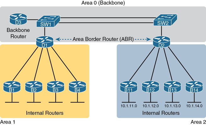
Figure 19-13 Three-Area OSPF with D1 and D2 as ABRs
The figure also shows a few important OSPF area design terms. Table 19-7 summarizes the meaning of these terms, plus some other related terms, but pay closest attention to the terms from the figure.
Table 19-7 OSPF Design Terminology
Term |
Description |
|---|---|
Area Border Router (ABR) |
An OSPF router with interfaces connected to the backbone area and to at least one other area |
Backbone router |
A router connected to the backbone area (includes ABRs) |
Internal router |
A router in one area (not the backbone area) |
Area |
A set of routers and links that shares the same detailed LSDB information, but not with routers in other areas, for better efficiency |
Backbone area |
A special OSPF area to which all other areas must connect—area 0 |
Intra-area route |
A route to a subnet inside the same area as the router |
Interarea route |
A route to a subnet in an area of which the router is not a part |
How Areas Reduce SPF Calculation Time
Figure 19-13 shows a sample area design and some terminology related to areas, but it does not show the power and benefit of the areas. To understand how areas reduce the work SPF has to do, you need to understand what changes about the LSDB inside an area, as a result of the area design.
SPF spends most of its processing time working through all the topology details, namely routers and the links that connect routers. Areas reduce SPF’s workload because, for a given area, the LSDB lists only routers and links inside that area, as shown on the left side of Figure 19-14.
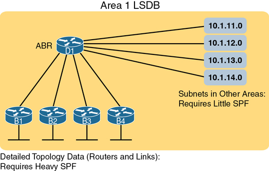
Figure 19-14 Smaller Area 1 LSDB Concept
While the LSDB has less topology information, it still has to have information about all subnets in all areas, so that each router can create IPv4 routes for all subnets. So, with an area design, OSPFv2 uses very brief summary information about the subnets in other areas. These summary LSAs do not include topology information about the other areas; however, each summary LSA does list a subnet ID and mask of a subnet in some other area. Summary LSAs do not require much SPF processing at all. Instead, these subnets all appear like subnets connected to the ABR (in Figure 19-14, ABR D1).
Using multiple areas improves OSPF operations in many ways for larger networks. The following list summarizes some of the key points arguing for the use of multiple areas in larger OSPF networks:
Routers require fewer CPU cycles to process the smaller per-area LSDB with the SPF algorithm, reducing CPU overhead and improving convergence time.
The smaller per-area LSDB requires less memory.
Changes in the network (for example, links failing and recovering) require SPF calculations only on routers in the area where the link changed state, reducing the number of routers that must rerun SPF.
Less information must be advertised between areas, reducing the bandwidth required to send LSAs.
(OSPFv2) Link-State Advertisements
Many people tend to get a little intimidated by OSPF LSAs when first learning about them. Commands that list a summary of the LSDB’s contents, like the show ip ospf database command, actually list a lot of information. Commands that list the details of the LSDB can list overwhelming amounts of information, and those details appear to be in some kind of code, using lots of numbers. It can seem like a bit of a mess.
However, if you examine LSAs while thinking about OSPF areas and area design, some of the most common LSA types will make a lot more sense. For instance, think about the LSDB in one area. The topology in one area includes routers and the links between the routers. As it turns out, OSPF defines the first two types of LSAs to define those exact details, as follows:
One router LSA for each router in the area
One network LSA for each network that has a DR plus one neighbor of the DR
Next, think about the subnets in the other areas. The ABR creates summary information about each subnet in one area to advertise into other areas—basically just the subnet IDs and masks—as a third type of LSA:
One summary LSA for each subnet ID that exists in a different area
The next few pages discuss these three LSA types in a little more detail; Table 19-8 lists some information about all three for easier reference and study.
Table 19-8 The Three OSPFv2 LSA Types Seen with a Multiarea OSPF Design
LSA Name |
LSA Type |
Primary Purpose |
Contents of LSA |
|---|---|---|---|
Router |
1 |
Describe a router |
RID, interfaces, IP address/mask, current interface state (status) |
Network |
2 |
Describe a network that has a DR |
DR and BDR IP addresses, subnet ID, mask |
Summary |
3 |
Describe a subnet in another area |
Subnet ID, mask, RID of ABR that advertises the LSA |
Router LSAs Build Most of the Intra-Area Topology
OSPF needs very detailed topology information inside each area. The routers inside area X need to know all the details about the topology inside area X. And the mechanism to give routers all these details is for the routers to create and flood router (Type 1) and network (Type 2) LSAs about the routers and links in the area.
Router LSAs, also known as Type 1 LSAs, describe the router in detail. Each lists a router’s RID, its interfaces, its IPv4 addresses and masks, its interface state, and notes about what neighbors the router knows about via each of its interfaces.
To see a specific instance, first review Figure 19-15. It lists internetwork topology, with subnets listed. Because it’s a small internetwork, the engineer chose a single-area design, with all interfaces in backbone area 0.
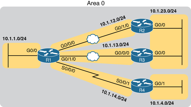
Figure 19-15 Enterprise Network with Seven IPv4 Subnets
With the single-area design planned for this small internetwork, the LSDB will contain four router LSAs. Each router creates a router LSA for itself, with its own RID as the LSA identifier. The LSA lists that router’s own interfaces, IP address/mask, with pointers to neighbors.
Once all four routers have copies of all four router LSAs, SPF can mathematically analyze the LSAs to create a model. The model looks a lot like the concept drawing in Figure 19-16. Note that the drawing shows each router with an obvious RID value. Each router has pointers that represent each of its interfaces, and because the LSAs identify neighbors, SPF can figure out which interfaces connect to which other routers.
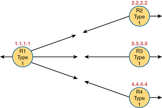
Figure 19-16 Type 1 LSAs, Assuming a Single-Area Design
Network LSAs Complete the Intra-Area Topology
Whereas router LSAs define most of the intra-area topology, network LSAs define the rest. As it turns out, when OSPF elects a DR on some subnet and that DR has at least one neighbor, OSPF treats that subnet as another node in its mathematical model of the network. To represent that network, the DR creates and floods a network (Type 2) LSA for that network (subnet).
For instance, back in Figure 19-15, one Ethernet LAN and two Ethernet WANs exist. The Ethernet LAN between R2 and R3 will elect a DR, and the two routers will become neighbors; so, whichever router is the DR will create a network LSA. Similarly, R1 and R2 connect with an Ethernet WAN, so the DR on that link will create a network LSA. Likewise, the DR on the Ethernet WAN link between R1 and R3 will also create a network LSA.
Figure 19-17 shows the completed version of the intra-area LSAs in area 0 with this design. Note that the router LSAs actually point to the network LSAs when they exist, which lets the SPF processes connect the pieces together.
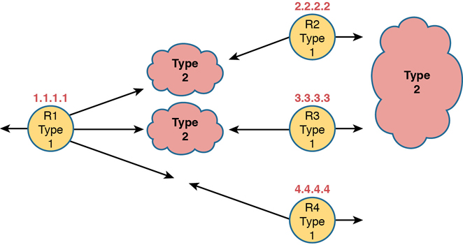
Figure 19-17 Type 1 and Type 2 LSAs in Area 0, Assuming a Single-Area Design
Finally, note that in this single-area design example no summary (Type 3) LSAs exist at all. These LSAs represent subnets in other areas, and there are no other areas. Given that the CCNA 200-301 exam topics refer specifically to single-area OSPF designs, this section stops at showing the details of the intra-area LSAs (Types 1 and 2).
Chapter Review
One key to doing well on the exams is to perform repetitive spaced review sessions. Review this chapter’s material using either the tools in the book or interactive tools for the same material found on the book’s companion website. Refer to the “Your Study Plan” element for more details. Table 19-9 outlines the key review elements and where you can find them. To better track your study progress, record when you completed these activities in the second column.
Table 19-9 Chapter Review Tracking
Review Element |
Review Date(s) |
Resource Used: |
|---|---|---|
Review key topics |
|
Book, website |
Review key terms |
|
Book, website |
Answer DIKTA questions |
|
Book, PTP |
Review memory tables |
|
Website |
Review All the Key Topics
Table 19-10 Key Topics for Chapter 19
Key Topic Element |
Description |
Page Number |
|---|---|---|
List |
Functions of IP routing protocols |
443 |
List |
Definitions of IGP and EGP |
444 |
List |
Types of IGP routing protocols |
446 |
IGP metrics |
446 |
|
List |
Key facts about the OSPF 2-way state |
453 |
Key OSPF neighbor states |
457 |
|
Item |
Definition of how OSPF calculates the cost for a route |
458 |
Example of calculating the cost for multiple competing routes |
458 |
|
List |
OSPF area design rules |
460 |
Sample OSPF multiarea design with terminology |
461 |
|
OSPF design terms and definitions |
461 |
Key Terms You Should Know
Shortest Path First (SPF) algorithm
Interior Gateway Protocol (IGP)
link-state advertisement (LSA)