Chapter 14. QoS
This chapter covers the following subjects:
The Need for QoS: This section describes the leading causes of poor quality of service and how they can be alleviated by using QoS tools and mechanisms.
QoS Models: This section describes the three different models available for implementing QoS in a network: best effort, Integrated Services (IntServ), and Differentiated Services (DiffServ).
Classification and Marking: This section describes classification, which is used to identify and assign IP traffic into different traffic classes, and marking, which is used to mark packets with a specified priority based on classification or traffic conditioning policies.
Policing and Shaping: This section describes how policing is used to enforce ratelimiting, where excess IP traffic is either dropped, marked, or delayed.
Congestion Management and Avoidance: This section describes congestion management, which is a queueing mechanism used to prioritize and protect IP traffic. It also describes congestion avoidance, which involves discarding IP traffic to avoid network congestion.
QoS is a network infrastructure technology that relies on a set of tools and mechanisms to assign different levels of priority to different IP traffic flows and provides special treatment to higher-priority IP traffic flows. For higher-priority IP traffic flows, it reduces packet loss during times of network congestion and also helps control delay (latency) and delay variation (jitter); for low-priority IP traffic flows, it provides a best-effort delivery service. This is analogous to how a high-occupancy vehicle (HOV) lane, also referred to as a carpool lane, works: A special high-priority lane is reserved for use of carpools (high-priority traffic), and those who carpool can flow freely by bypassing the heavy traffic congestion in the adjacent general-purpose lanes.
These are the primary goals of implementing QoS on a network:
Expediting delivery for real-time applications
Ensuring business continuance for business-critical applications
Providing fairness for non-business-critical applications when congestion occurs
Establishing a trust boundary across the network edge to either accept or reject traffic markings injected by the endpoints
QoS uses the following tools and mechanisms to achieve its goals:
Classification and marking
Policing and shaping
Congestion management and avoidance
All of these QoS mechanisms are described in this chapter.
“Do I Know This Already?” Quiz
The “Do I Know This Already?” quiz allows you to assess whether you should read the entire chapter. If you miss no more than one of these self-assessment questions, you might want to move ahead to the “Exam Preparation Tasks” section. Table 14-1 lists the major headings in this chapter and the “Do I Know This Already?” quiz questions covering the material in those headings so you can assess your knowledge of these specific areas. The answers to the “Do I Know This Already?” quiz appear in Appendix A, “Answers to the ‘Do I Know This Already?’ Quiz Questions.”
Table 14-1 “Do I Know This Already?” Foundation Topics Section-to-Question Mapping
Foundation Topics Section |
Questions |
The Need for QoS |
1–2 |
QoS Models |
3–5 |
Classification and Marking |
6–9 |
Policing and Shaping |
10–11 |
Congestion Management and Avoidance |
12–13 |
1. Which of the following are the leading causes of quality of service issues?(Choose all that apply.)
Bad hardware
Lack of bandwidth
Latency and jitter
Copper cables
Packet loss
2. Network latency can be broken down into which of the following types?(Choose all that apply.)
Propagation delay (fixed)
Time delay (variable)
Serialization delay (fixed)
Processing delay (fixed)
Packet delay (fixed)
Delay variation (variable)
3. Which of the following is not a QoS implementation model?
IntServ
Expedited forwarding
Best effort
DiffServ
4. Which of the following is the QoS implementation model that requires a signaling protocol?
IntServ
Best Effort
DiffServ
RSVP
5. Which of the following is the most popular QoS implementation model?
IntServ
Best effort
DiffServ
RSVP
6. True or false: Traffic classification should always be performed in the core of the network.
True
False
7. The 16-bit TCI field is composed of which fields? (Choose three.)
Priority Code Point (PCP)
Canonical Format Identifier (CFI)
User Priority (PRI)
Drop Eligible Indicator (DEI)
VLAN Identifier (VLAN ID)
8. True or false: The DiffServ field is an 8-bit Differentiated Services Code Point (DSCP) field that allows for classification of up to 64 values (0 to 63).
True
False
9. Which of the following is not a QoS PHB?
Best Effort (BE)
Class Selector (CS)
Default Forwarding (DF)
Assured Forwarding (AF)
Expedited Forwarding (EF)
10. Which traffic conditioning tool can be used to drop or mark down traffic that goes beyond a desired traffic rate?
Policers
Shapers
WRR
None of the above
11. What does Tc stand for? (Choose two.)
Committed time interval
Token credits
Bc bucket token count
Traffic control
12. Which of the following are the recommended congestion management mechanisms for modern rich-media networks? (Choose two.)
Class-based weighted fair queuing (CBWFQ)
Priority queuing (PQ)
Weighted RED (WRED)
Low-latency queuing (LLQ)
13. Which of the following is a recommended congestion-avoidance mechanism for modern rich-media networks?
Weighted RED (WRED)
Tail drop
FIFO
RED
Answers to the “Do I Know This Already?” quiz:
1 B, C, E
2 A, C, D, F
3 B
4 A
5 C
6 B
7 A, D, E
8 B
9 A
10 A
11 A, C
12 A, D
13 A
Foundation Topics
The Need for QoS
Modern real-time multimedia applications such as IP telephony, telepresence, broadcast video, Cisco Webex, and IP video surveillance are extremely sensitive to delivery delays and create unique quality of service (QoS) demands on a network. When packets are delivered using a best-effort delivery model, they may not arrive in order or in a timely manner, and they may be dropped. For video, this can result in pixelization of the image, pausing, choppy video, audio and video being out of sync, or no video at all. For audio, it could cause echo, talker overlap (a walkie-talkie effect where only one person can speak at a time), unintelligible and distorted speech, voice breakups, longs silence gaps, and call drops. The following are the leading causes of quality issues:
Lack of bandwidth
Latency and jitter
Packet loss
Lack of Bandwidth
The available bandwidth on the data path from a source to a destination equals the capacity of the lowest-bandwidth link. When the maximum capacity of the lowest-bandwidth link is surpassed, link congestion takes place, resulting in traffic drops. The obvious solution to this type of problem is to increase the link bandwidth capacity, but this is not always possible, due to budgetary or technological constraints. Another option is to implement QoS mechanisms such as policing and queueing to prioritize traffic according to level of importance. Voice, video, and business-critical traffic should get prioritized forwarding and sufficient bandwidth to support their application requirements, and the least important traffic should be allocated the remaining bandwidth.
Latency and Jitter
One-way end-to-end delay, also referred to as network latency, is the time it takes for packets to travel across a network from a source to a destination. ITU Recommendation G.114 recommends that, regardless of the application type, a network latency of 400 ms should not be exceeded, and for real-time traffic, network latency should be less than 150 ms; however, ITU and Cisco have demonstrated that real-time traffic quality does not begin to significantly degrade until network latency exceeds 200 ms. To be able to implement these recommendations, it is important to understand what causes network latency. Network latency can be broken down into fixed and variable latency:
Propagation delay (fixed)
Serialization delay (fixed)
Processing delay (fixed)
Delay variation (variable)
Propagation Delay
Propagation delay is the time it takes for a packet to travel from the source to a destination at the speed of light over a medium such as fiber-optic cables or copper wires. The speed of light is 299,792,458 meters per second in a vacuum. The lack of vacuum conditions in a fiber-optic cable or a copper wire slows down the speed of light by a ratio known as the refractive index; the larger the refractive index value, the slower light travels.
The average refractive index value of an optical fiber is about 1.5. The speed of light through a medium v is equal to the speed of light in a vacuum c divided by the refractive index n, or v = c / n. This means the speed of light through a fiber-optic cable with a refractive index of 1.5 is approximately 200,000,000 meters per second (that is, 300,000,000 / 1.5).
If a single fiber-optic cable with a refractive index of 1.5 were laid out around the equatorial circumference of Earth, which is about 40,075 km, the propagation delay would be equal to the equatorial circumference of Earth divided by 200,000,000 meters per second. This is approximately 200 ms, which would be an acceptable value even for real-time traffic.
Keep in mind that optical fibers are not always physically placed over the shortest path between two points. Fiber-optic cables may be hundreds or even thousands of miles longer than expected. In addition, other components required by fiber-optic cables, such as repeaters and amplifiers, may introduce additional delay. A provider’s service-level agreement (SLA) can be reviewed to estimate and plan for the minimum, maximum, and average latency for a circuit.
Serialization Delay
Serialization delay is the time it takes to place all the bits of a packet onto a link. It is a fixed value that depends on the link speed; the higher the link speed, the lower the delay. The serialization delay s is equal to the packet size in bits divided by the line speed in bits per second. For example, the serialization delay for a 1500-byte packet over a 1 Gbps interface is 12 μs and can be calculated as follows:
s = packet size in bits / line speed in bps
s = (1500 bytes × 8) / 1 Gbps
s = 12,000 bits / 1000,000,000 bps = 0.000012 s × 1000 = .012 ms × 1000 = 12 μs
Processing Delay
Processing delay is the fixed amount of time it takes for a networking device to take the packet from an input interface and place the packet onto the output queue of the output interface. The processing delay depends on factors such as the following:
CPU speed (for software-based platforms)
CPU utilization (load)
IP packet switching mode (process switching, software CEF, or hardware CEF)
Router architecture (centralized or distributed)
Configured features on both input and output interfaces
Delay Variation
Delay variation, also referred to as jitter, is the difference in the latency between packets in a single flow. For example, if one packet takes 50 ms to traverse the network from the source to destination, and the following packet takes 70 ms, the jitter is 20 ms. The major factors affecting variable delays are queuing delay, dejitter buffers, and variable packet sizes.
Jitter is experienced due to the queueing delay experienced by packets during periods of network congestion. Queuing delay depends on the number and sizes of packets already in the queue, the link speed, and the queuing mechanism. Queuing introduces unequal delays for packets of the same flow, thus producing jitter.
Voice and video endpoints typically come equipped with de-jitter buffers that can help smooth out changes in packet arrival times due to jitter. A de-jitter buffer is often dynamic and can adjust for approximately 30 ms changes in arrival times of packets. If a packet is not received within the 30 ms window allowed for by the de-jitter buffer, the packet is dropped, and this affects the overall voice or video quality.
To prevent jitter for high-priority real-time traffic, it is recommended to use queuing mechanisms such as low-latency queueing (LLQ) that allow matching packets to be forwarded prior to any other low priority traffic during periods of network congestion.
Packet Loss
Packet loss is usually a result of congestion on an interface. Packet loss can be prevented by implementing one of the following approaches:
Increase link speed.
Implement QoS congestion-avoidance and congestion-management mechanism.
Implement traffic policing to drop low-priority packets and allow high-priority traffic through.
Implement traffic shaping to delay packets instead of dropping them since traffic may burst and exceed the capacity of an interface buffer. Traffic shaping is not recommended for real-time traffic because it relies on queuing that can cause jitter.
QoS Models
There are three different QoS implementation models:
Best effort: QoS is not enabled for this model. It is used for traffic that does not require any special treatment.
Integrated Services (IntServ): Applications signal the network to make a bandwidth reservation and to indicate that they require special QoS treatment.
Differentiated Services (DiffServ): The network identifies classes that require special QoS treatment.
The IntServ model was created for real-time applications such as voice and video that require bandwidth, delay, and packet-loss guarantees to ensure both predictable and guaranteed service levels. In this model, applications signal their requirements to the network to reserve the end-to-end resources (such as bandwidth) they require to provide an acceptable user experience. IntServ uses Resource Reservation Protocol (RSVP) to reserve resources throughout a network for a specific application and to provide call admission control (CAC) to guarantee that no other IP traffic can use the reserved bandwidth. The bandwidth reserved by an application that is not being used is wasted.
To be able to provide end-to-end QoS, all nodes, including the endpoints running the applications, need to support, build, and maintain RSVP path state for every single flow. This is the biggest drawback of IntServ because it means it cannot scale well on large networks that might have thousands or millions of flows due to the large number of RSVP flows that would need to be maintained.
Figure 14-1 illustrates how RSVP hosts issue bandwidth reservations.
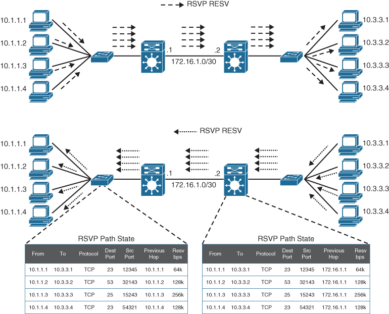
Figure 14-1 RSVP Reservation Establishment
In Figure 14-1, each of the hosts on the left side (senders) are attempting to establish aone-to-one bandwidth reservation to each of the hosts on the right side (receivers). The senders start by sending RSVP PATH messages to the receivers along the same path used by regular data packets. RSVP PATH messages carry the receiver source address, the destination address, and the bandwidth they wish to reserve. This information is stored in the RSVP path state of each node. Once the RSVP PATH messages reach the receivers, each receiver sends RSVP reservation request (RESV) messages in the reverse path of the data flow toward the receivers, hop-by-hop. At each hop, the IP destination address of a RESV message is the IP address of the previous-hop node, obtained from the RSVP path state of each node. As RSVP RESV messages cross each hop, they reserve bandwidth on each of the links for the traffic flowing from the receiver hosts to the sender hosts. If bandwidth reservations are required from the hosts on the right side to the hosts on the left side, the hosts on the right side need to follow the same procedure of sending RSVP PATH messages, which doubles the RSVP state on each networking device in the data path. This demonstrates how RSVP state can increase quickly as more hosts reserve bandwidth. Apart from the scalability issues, long distances between hosts could also trigger long bandwidth reservation delays.
DiffServ was designed to address the limitations of the best-effort and IntServ models. With this model, there is no need for a signaling protocol, and there is no RSVP flow state to maintain on every single node, which makes it highly scalable; QoS characteristics (such as bandwidth and delay) are managed on a hop-by-hop basis with QoS policies that are defined independently at each device in the network. DiffServ is not considered an end-to-end QoS solution because end-to-end QoS guarantees cannot be enforced.
DiffServ divides IP traffic into classes and marks it based on business requirements so that each of the classes can be assigned a different level of service. As IP traffic traverses a network, each of the network devices identifies the packet class by its marking and services the packets according to this class. Many levels of service can be chosen with DiffServ. For example, IP phone voice traffic is very sensitive to latency and jitter, so it should always be given preferential treatment over all other application traffic. Email, on the other hand, can withstand a great deal of delay and could be given best-effort service, and non-business, non-critical scavenger traffic (such as from YouTube) can either be heavily rate limited or blocked entirely. The DiffServ model is the most popular and most widely deployed QoS model and is covered in detail in this chapter.
Classification and Marking
Before any QoS mechanism can be applied, IP traffic must first be identified and categorized into different classes, based on business requirements. Network devices use classification to identify IP traffic as belonging to a specific class. After the IP traffic is classified, marking can be used to mark or color individual packets so that other network devices can apply QoS mechanisms to those packets as they traverse the network. This section introduces the concepts of classification and marking, explains the different marking options that are available for Layer 2 frames and Layer 3 packets, and explains where classification and marking tools should be used in a network.
Classification
Packet classification is a QoS mechanism responsible for distinguishing between different traffic streams. It uses traffic descriptors to categorize an IP packet within a specific class. Packet classification should take place at the network edge, as close to the source of the traffic as possible. Once an IP packet is classified, packets can then be marked/re-marked, queued, policed, shaped, or any combination of these and other actions.
The following traffic descriptors are typically used for classification:
Internal: QoS groups (locally significant to a router)
Layer 1: Physical interface, subinterface, or port
Layer 2: MAC address and 802.1Q/p Class of Service (CoS) bits
Layer 2.5: MPLS Experimental (EXP) bits
Layer 3: Differentiated Services Code Points (DSCP), IP Precedence (IPP), and source/destination IP address
Layer 4: TCP or UDP ports
Layer 7: Next Generation Network-Based Application Recognition (NBAR2)
For enterprise networks, the most commonly used traffic descriptors used for classification include the Layer 2, Layer 3, Layer 4, and Layer 7 traffic descriptors listed here. The following section explores the Layer 7 traffic descriptor NBAR2.
Layer 7 Classification
NBAR2 is a deep packet inspection engine that can classify and identify a wide variety of protocols and applications using Layer 3 to Layer 7 data, including difficult-to-classify applications that dynamically assign Transmission Control Protocol (TCP) or User Datagram Protocol (UDP) port numbers.
NBAR2 can recognize more than 1000 applications, and monthly protocol packs are provided for recognition of new and emerging applications, without requiring an IOS upgrade or router reload.
NBAR2 has two modes of operation:
Protocol Discovery: Protocol Discovery enables NBAR2 to discover and get real-time statistics on applications currently running in the network. These statistics from the Protocol Discovery mode can be used to define QoS classes and policies using MQC configuration.
Modular QoS CLI (MQC): Using MQC, network traffic matching a specific network protocol such as Cisco Webex can be placed into one traffic class, while traffic that matches a different network protocol such as YouTube can be placed into another traffic class. After traffic has been classified in this way, different QoS policies can be applied to the different classes of traffic.
Marking
Packet marking is a QoS mechanism that colors a packet by changing a field within a packet or a frame header with a traffic descriptor so it is distinguished from other packets during the application of other QoS mechanisms (such as re-marking, policing, queuing, or congestion avoidance).
The following traffic descriptors are used for marking traffic:
Internal: QoS groups
Layer 2: 802.1Q/p Class of Service (CoS) bits
Layer 2.5: MPLS Experimental (EXP) bits
Layer 3: Differentiated Services Code Points (DSCP) and IP Precedence (IPP)
For enterprise networks, the most commonly used traffic descriptors for marking traffic include the Layer 2 and Layer 3 traffic descriptors mentioned in the previous list. Both of them are described in the following sections.
Layer 2 Marking
The 802.1Q standard is an IEEE specification for implementing VLANs in Layer 2 switched networks. The 802.1Q specification defines two 2-byte fields: Tag Protocol Identifier (TPID) and Tag Control Information (TCI), which are inserted within an Ethernet frame following the Source Address field, as illustrated in Figure 14-2.
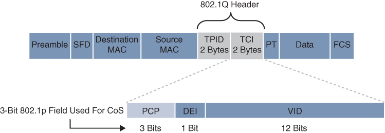
Figure 14-2 802.1Q Layer 2 QoS Using 802.1p CoS
The TPID value is a 16-bit field assigned the value 0x8100 that identifies it as an 802.1Q tagged frame.
The TCI field is a 16-bit field composed of the following three fields:
Priority Code Point (PCP) field (3 bits)
Drop Eligible Indicator (DEI) field (1 bit)
VLAN Identifier (VLAN ID) field (12 bits)
Priority Code Point (PCP)
The specifications of the 3-bit PCP field are defined by the IEEE 802.1p specification. This field is used to mark packets as belonging to a specific CoS. The CoS marking allows a Layer 2 Ethernet frame to be marked with eight different levels of priority values, 0 to 7,where 0 is the lowest priority and 7 is the highest. Table 14-2 includes the IEEE 802.1p specification standard definition for each CoS.
Table 14-2 IEEE 802.1p CoS Definitions
PCP Value/Priority |
Acronym |
Traffic Type |
0 (lowest) |
BK |
Background |
1 (default) |
BE |
Best effort |
2 |
EE |
Excellent effort |
3 |
CA |
Critical applications |
4 |
VI |
Video with < 100 ms latency and jitter |
5 |
VO |
Voice with < 10 ms latency and jitter |
6 |
IC |
Internetwork control |
7 (highest) |
NC |
Network control |
One drawback of using CoS markings is that frames lose their CoS markings when traversing a non-802.1Q link or a Layer 3 network. For this reason, packets should be marked with other higher-layer markings whenever possible so the marking values can be preserved end-to-end. This is typically accomplished by mapping a CoS marking into another marking. For example, the CoS priority levels correspond directly to IPv4’s IP Precedence Type of Service (ToS) values so they can be mapped directly to each other.
Drop Eligible Indicator (DEI)
The DEI field is a 1-bit field that can be used independently or in conjunction with PCP to indicate frames that are eligible to be dropped during times of congestion. The default value for this field is 0, and it indicates that this frame is not drop eligible; it can be set to 1 to indicate that the frame is drop eligible.
VLAN Identifier (VLAN ID)
The VLAN ID field is a 12-bit field that defines the VLAN used by 802.1Q. Since this field is 12 bits, it restricts the number of VLANs supported by 802.1Q to 4096, which may not be sufficient for large enterprise or service provider networks.
Layer 3 Marking
As a packet travels from its source to its destination, it might traverse non-802.1Q trunked, or non-Ethernet links that do not support the CoS field. Using marking at Layer 3 provides a more persistent marker that is preserved end-to-end.
Figure 14-3 illustrates the ToS/DiffServ field within an IPv4 header.
Figure 14-3 IPv4 ToS/DiffServ Field
The ToS field is an 8-bit field where only the first 3 bits of the ToS field, referred to as IP Precedence (IPP), are used for marking, and the rest of the bits are unused. IPP values, which range from 0 to 7, allow the traffic to be partitioned in up to six usable classes of service; IPP 6 and 7 are reserved for internal network use.
Newer standards have redefined the IPv4 ToS and the IPv6 Traffic Class fields as an 8-bit Differentiated Services (DiffServ) field. The DiffServ field uses the same 8 bits that were previously used for the IPv4 ToS and the IPv6 Traffic Class fields, and this allows it to be backward compatible with IP Precedence. The DiffServ field is composed of a 6-bit Differentiated Services Code Point (DSCP) field that allows for classification of up to64 values (0 to 63) and a 2-bit Explicit Congestion Notification (ECN) field.
DSCP Per-Hop Behaviors
Packets are classified and marked to receive a particular per-hop forwarding behavior (that is, expedited, delayed, or dropped) on network nodes along their path to the destination. The DiffServ field is used to mark packets according to their classification into DiffServ Behavior Aggregates (BAs). A DiffServ BA is a collection of packets with the same DiffServ value crossing a link in a particular direction. Per-hop behavior (PHB) is the externally observable forwarding behavior (forwarding treatment) applied at a DiffServ-compliant node to a collection of packets with the same DiffServ value crossing a link in a particular direction (DiffServ BA).
In other words, PHB is expediting, delaying, or dropping a collection of packets by one or multiple QoS mechanisms on a per-hop basis, based on the DSCP value. A DiffServ BA could be multiple applications—for example, SSH, Telnet, and SNMP all aggregated together and marked with the same DSCP value. This way, the core of the network performs only simple PHB, based on DiffServ BAs, while the network edge performs classification, marking, policing, and shaping operations. This makes the DiffServ QoS model very scalable.
Four PHBs have been defined and characterized for general use:
Class Selector (CS) PHB: The first 3 bits of the DSCP field are used as CS bits. The CS bits make DSCP backward compatible with IP Precedence because IP Precedence uses the same 3 bits to determine class.
Default Forwarding (DF) PHB: Used for best-effort service.
Assured Forwarding (AF) PHB: Used for guaranteed bandwidth service.
Expedited Forwarding (EF) PHB: Used for low-delay service.
Class Selector (CS) PHB
RFC 2474 made the ToS field obsolete by introducing the DiffServ field, and the Class Selector (CS) PHB was defined to provide backward compatibility for DSCP with IP Precedence. Figure 14-4 illustrates the CS PHB.
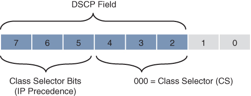
Figure 14-4 Class Selector (CS) PHB
Packets with higher IP Precedence should be forwarded in less time than packets with lower IP Precedence.
The last 3 bits of the DSCP (bits 2 to 4), when set to 0, identify a Class Selector PHB, but the Class Selector bits 5 to 7 are the ones where IP Precedence is set. Bits 2 to 4 are ignored by non-DiffServ-compliant devices performing classification based on IP Precedence.
There are eight CS classes, ranging from CS0 to CS7, that correspond directly with the eight IP Precedence values.
Default Forwarding (DF) PHB
Default Forwarding (DF) and Class Selector 0 (CS0) provide best-effort behavior and use the DS value 000000. Figure 14-5 illustrates the DF PHB.
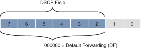
Figure 14-5 Default Forwarding (DF) PHB
Default best-effort forwarding is also applied to packets that cannot be classified by a QoS mechanism such as queueing, shaping, or policing. This usually happens when a QoS policy on the node is incomplete or when DSCP values are outside the ones that have been defined for the CS, AF, and EF PHBs.
Assured Forwarding (AF) PHB
The AF PHB guarantees a certain amount of bandwidth to an AF class and allows access to extra bandwidth, if available. Packets requiring AF PHB should be marked with DSCP value aaadd0, where aaa is the binary value of the AF class (bits 5 to 7), and dd (bits 2 to 4) is the drop probability where bit 2 is unused and always set to 0. Figure 14-6 illustrates the AF PHB.
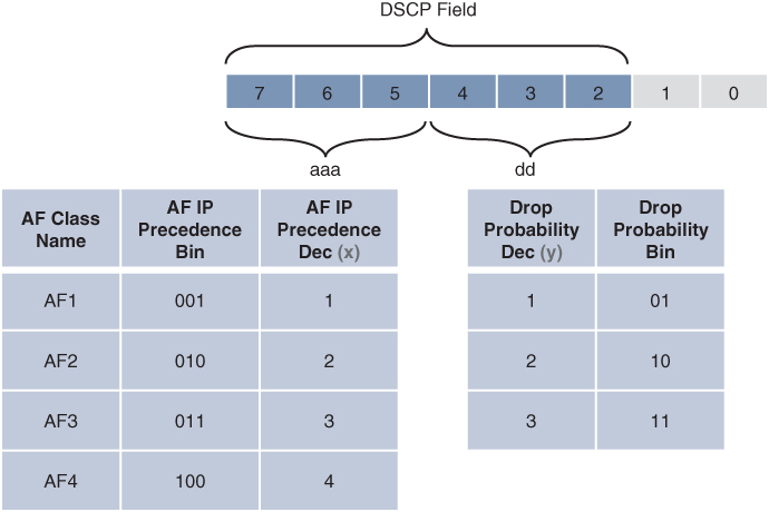
Figure 14-6 Assured Forwarding (AF) PHB
There are four standard-defined AF classes: AF1, AF2, AF3, and AF4. The AF class number does not represent precedence; for example, AF4 does not get any preferential treatment over AF1. Each class should be treated independently and placed into different queues.
Table 14-3 illustrates how each AF class is assigned an IP Precedence (under AF Class Value Bin) and has three drop probabilities: low, medium, and high.
The AF Name (AFxy) is composed of the AF IP Precedence value in decimal (x) and the Drop Probability value in decimal (y). For example, AF41 is a combination of IP Precedence 4 and Drop Probability 1.
To quickly convert the AF Name into a DSCP value in decimal, use the formula 8x + 2y. For example, the DSCP value for AF41 is 8(4) + 2(1) = 34.
Table 14-3 AF PHBs with Decimal and Binary Equivalents
AF Class Name |
AF IP Precedence Dec (x) |
AF IP Precedence Bin |
Drop Probability |
Drop Probability Value Bin |
Drop Probability Value Dec (y) |
AF Name (AFxy) |
DSCP Value Bin |
DSCP Value Dec |
AF1 |
1 |
001 |
Low |
01 |
1 |
AF11 |
001010 |
10 |
AF1 |
1 |
001 |
Medium |
10 |
2 |
AF12 |
001100 |
12 |
AF1 |
1 |
001 |
High |
11 |
3 |
AF13 |
001110 |
14 |
AF2 |
2 |
010 |
Low |
01 |
1 |
AF21 |
010010 |
18 |
AF2 |
2 |
010 |
Medium |
10 |
2 |
AF22 |
010100 |
20 |
AF2 |
2 |
010 |
High |
11 |
3 |
AF23 |
010110 |
22 |
AF3 |
3 |
011 |
Low |
01 |
1 |
AF31 |
011010 |
26 |
AF3 |
3 |
011 |
Medium |
10 |
2 |
AF32 |
011100 |
28 |
AF3 |
3 |
011 |
High |
11 |
3 |
AF33 |
011110 |
30 |
AF4 |
4 |
100 |
Low |
01 |
1 |
AF41 |
100010 |
34 |
AF4 |
4 |
100 |
Medium |
10 |
2 |
AF42 |
100100 |
36 |
AF4 |
4 |
100 |
High |
11 |
3 |
AF43 |
100110 |
38 |
An AF implementation must detect and respond to long-term congestion within each class by dropping packets using a congestion-avoidance algorithm such as weighted random early detection (WRED). WRED uses the AF Drop Probability value within each class—where 1 is the lowest possible value, and 3 is the highest possible—to determine which packets should be dropped first during periods of congestion. It should also be able to handle short-term congestion resulting from bursts if each class is placed in a separate queue, using a queueing algorithm such as class-based weighted fair queueing (CBWFQ). The AF specification does not define the use of any particular algorithms to use for queueing and congestions avoidance, but it does specify the requirements and properties of such algorithms.
Expedited Forwarding (EF) PHB
The EF PHB can be used to build a low-loss, low-latency, low-jitter, assured bandwidth, end-to-end service. The EF PHB guarantees bandwidth by ensuring a minimum departure rate and provides the lowest possible delay to delay-sensitive applications by implementing low-latency queueing. It also prevents starvation of other applications or classes that are not using the EF PHB by policing EF traffic when congestion occurs.
Packets requiring EF should be marked with DSCP binary value 101110 (46 in decimal). Bits 5 to 7 (101) of the EF DSCP value map directly to IP Precedence 5 for backward compatibility with non-DiffServ-compliant devices. IP Precedence 5 is the highest user-definable IP Precedence value and is used for real-time delay-sensitive traffic (such as VoIP).
Table 14-4 includes all the DSCP PHBs (DF, CS, AF, and EF) with their decimal and binary equivalents. This table can also be used to see which IP Precedence value corresponds to each PHB.
Table 14-4 DSCP PHBs with Decimal and Binary Equivalents and IPP
DSCP Class |
DSCP Value Bin |
Decimal Value Dec |
Drop Probability |
Equivalent IP Precedence Value |
DF (CS0) |
000 000 |
0 |
|
0 |
CS1 |
001 000 |
8 |
|
1 |
AF11 |
001 010 |
10 |
Low |
1 |
AF12 |
001 100 |
12 |
Medium |
1 |
AF13 |
001 110 |
14 |
High |
1 |
CS2 |
010 000 |
16 |
|
2 |
AF21 |
010 010 |
18 |
Low |
2 |
AF22 |
010 100 |
20 |
Medium |
2 |
AF23 |
010 110 |
22 |
High |
2 |
CS3 |
011 000 |
24 |
|
3 |
AF31 |
011 010 |
26 |
Low |
3 |
AF32 |
011 100 |
28 |
Medium |
3 |
AF33 |
011 110 |
30 |
High |
3 |
CS4 |
100 000 |
32 |
|
4 |
AF41 |
100 010 |
34 |
Low |
4 |
AF42 |
100 100 |
36 |
Medium |
4 |
AF43 |
100 110 |
38 |
High |
4 |
CS5 |
101 000 |
40 |
|
5 |
EF |
101 110 |
46 |
|
5 |
CS6 |
110 000 |
48 |
|
6 |
CS7 |
111 000 |
56 |
|
7 |
Scavenger Class
The scavenger class is intended to provide less than best-effort services. Applications assigned to the scavenger class have little or no contribution to the business objectives of an organization and are typically entertainment-related applications. These include peer-to-peer applications (such as Torrent), gaming applications (for example, Minecraft, Fortnite), and entertainment video applications (for example, YouTube, Vimeo, Netflix). These types of applications are usually heavily rate limited or blocked entirely.
Something very peculiar about the scavenger class is that it is intended to be lower in priority than a best-effort service. Best-effort traffic uses a DF PHB with a DSCP value of 000000 (CS0). Since there are no negative DSCP values, it was decided to use CS1 as the marking for scavenger traffic. This is defined in RFC 4594.
Trust Boundary
To provide an end-to-end and scalable QoS experience, packets should be marked by the endpoint or as close to the endpoint as possible. When an endpoint marks a frame or a packet with a CoS or DSCP value, the switch port it is attached to can be configured to accept or reject the CoS or DSCP values. If the switch accepts the values, it means it trusts the endpoint and does not need to do any packet reclassification and re-marking for the received endpoint’s packets. If the switch does not trust the endpoint, it rejects the markings and reclassifies and re-marks the received packets with the appropriate CoS or DSCP value.
For example, consider a campus network with IP telephony and host endpoints; the IP phones by default mark voice traffic with a CoS value of 5 and a DSCP value of 46 (EF), while incoming traffic from an endpoint (such as a PC) attached to the IP phone’s switch port is re-marked to a CoS value of 0 and a DSCP value of 0. Even if the endpoint is sending tagged frames with a specific CoS or DSCP value, the default behavior for Cisco IP phones is to not trust the endpoint and zero out the CoS and DSCP values before sending the frames to the switch. When the IP phone sends voice and data traffic to the switch, the switch can classify voice traffic as higher priority than the data traffic, thanks to the high-priority CoS and DSCP markings for voice traffic.
For scalability, trust boundary classification should be done as close to the endpoint as possible. Figure 14-7 illustrates trust boundaries at different points in a campus network, where 1 and 2 are optimal, and 3 is acceptable only when the access switch is not capable of performing classification.

Figure 14-7 Trust Boundaries
A Practical Example: Wireless QoS
A wireless network can be configured to leverage the QoS mechanisms described in this chapter. For example, a wireless LAN controller (WLC) sits at the boundary between wireless and wired networks, so it becomes a natural location for a QoS trust boundary. Traffic entering and exiting the WLC can be classified and marked so that it can be handled appropriately as it is transmitted over the air and onto the wired network.
Wireless QoS can be uniquely defined on each wireless LAN (WLAN), using the four traffic categories listed in Table 14-5. Notice that the category names are human-readable words that translate to specific 802.1p and DSCP values.
Table 14-5 Wireless QoS Policy Categories and Markings
QoS Category |
Traffic Type |
802.1p Tag |
DSCP Value |
Platinum |
Voice |
5 |
46 (EF) |
Gold |
Video |
4 |
34 (AF41) |
Silver |
Best effort (default) |
0 |
0 |
Bronze |
Background |
1 |
10 (AF11) |
When you create a new WLAN, its QoS policy defaults to Silver, or best-effort handling. In Figure 14-8, a WLAN named ‘voice’ has been created to carry voice traffic, so its QoS policy has been set to Platinum. Wireless voice traffic will then be classified for low latency and low jitter and marked with an 802.1p CoS value of 5 and a DSCP value of 46 (EF).
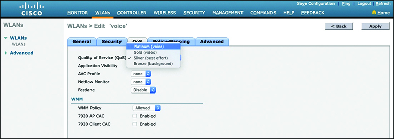
Figure 14-8 Setting the QoS Policy for a Wireless LAN
Policing and Shaping
Traffic policers and shapers are traffic-conditioning QoS mechanisms used to classify traffic and enforce other QoS mechanisms such as rate limiting. They classify traffic in an identical manner but differ in their implementation:
Policers: Drop or re-mark incoming or outgoing traffic that goes beyond a desired traffic rate.
Shapers: Buffer and delay egress traffic rates that momentarily peak above the desired rate until the egress traffic rate drops below the defined traffic rate. If the egress traffic rate is below the desired rate, the traffic is sent immediately.
Figure 14-9 illustrates the difference between traffic policing and shaping. Policers drop or re-mark excess traffic, while shapers buffer and delay excess traffic.

Figure 14-9 Policing Versus Shaping
Placing Policers and Shapers in the Network
Policers for incoming traffic are most optimally deployed at the edge of the network to keep traffic from wasting valuable bandwidth in the core of the network. Policers for outbound traffic are most optimally deployed at the edge of the network or core-facing interfaces on network edge devices. A downside of policing is that it causes TCP retransmissions when it drops traffic.
Shapers are used for egress traffic and typically deployed by enterprise networks on service provider (SP)–facing interfaces. Shaping is useful in cases where SPs are policing incoming traffic or when SPs are not policing traffic but do have a maximum traffic rate SLA, which, if violated, could incur monetary penalties. Shaping buffers and delays traffic rather than dropping it, and this causes fewer TCP retransmissions compared to policing.
Markdown
When a desired traffic rate is exceeded, a policer can take one of the following actions:
Drop the traffic.
Mark down the excess traffic with a lower priority.
Marking down excess traffic involves re-marking the packets with a lower-priority class value; for example, excess traffic marked with AFx1 should be marked down to AFx2 (or AFx3 if using two-rate policing). After marking down the traffic, congestion-avoidance mechanisms, such as DSCP-based weighted random early detection (WRED), should be configured throughout the network to drop AFx3 more aggressively than AFx2 and drop AFx2 more aggressively than AFx1.
Token Bucket Algorithms
Cisco IOS policers and shapers are based on token bucket algorithms. The following list includes definitions that are used to explain how token bucket algorithms operate:
Committed Information Rate (CIR): The policed traffic rate, in bits per second (bps), defined in the traffic contract.
Committed Time Interval (Tc): The time interval, in milliseconds (ms), over which the committed burst (Bc) is sent. Tc can be calculated with the formula Tc = (Bc [bits] / CIR [bps]) × 1000.
Committed Burst Size (Bc): The maximum size of the CIR token bucket, measured in bytes, and the maximum amount of traffic that can be sent within a Tc. Bc can be calculated with the formula Bc = CIR × (Tc / 1000).
Token: A single token represents 1 byte or 8 bits.
Token bucket: A bucket that accumulates tokens until a maximum predefined number of tokens is reached (such as the Bc when using a single token bucket); these tokens are added into the bucket at a fixed rate (the CIR). Each packet is checked for conformance to the defined rate and takes tokens from the bucket equal to its packet size; for example, if the packet size is 1500 bytes, it takes 12,000 bits (1500 × 8) from the bucket. If there are not enough tokens in the token bucket to send the packet, the traffic conditioning mechanism can take one of the following actions:
Buffer the packets while waiting for enough tokens to accumulate in the token bucket (traffic shaping)
Drop the packets (traffic policing)
Mark down the packets (traffic policing)
It is recommended for the Bc value to be larger than or equal to the size of the largest possible IP packet in a traffic stream. Otherwise, there will never be enough tokens in the token bucket for larger packets, and they will always exceed the defined rate. If the bucket fills up to the maximum capacity, newly added tokens are discarded. Discarded tokens are not available for use in future packets.
Token bucket algorithms may use one or multiple token buckets. For single token bucket algorithms, the measured traffic rate can conform to or exceed the defined traffic rate. The measured traffic rate is conforming if there are enough tokens in the token bucket to transmit the traffic. The measured traffic rate is exceeding if there are not enough tokens in the token bucket to transmit the traffic.
Figure 14-10 illustrates the concept of the single token bucket algorithm.
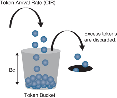
Figure 14-10 Single Token Bucket Algorithm
To understand how the single token bucket algorithms operate in more detail, assume that a 1 Gbps interface is configured with a policer defined with a CIR of 120 Mbps and a Bc of 12 Mb. The Tc value cannot be explicitly defined in IOS, but it can be calculated as follows:
Tc = (Bc [bits] / CIR [bps]) × 1000
Tc = (12 Mb / 120 Mbps) × 1000
Tc = (12,000,000 bits / 120,000,000 bps) × 1000 = 100 ms
Once the Tc value is known, the number of Tcs within a second can be calculated as follows:
Tcs per second = 1000 / Tc
Tcs per second = 1000 ms / 100 ms = 10 Tcs
If a continuous stream of 1500-byte (12,000-bit) packets is processed by the token algorithm, only a Bc of 12 Mb can be taken by the packets within each Tc (100 ms). The number of packets that conform to the traffic rate and are allowed to be transmitted can be calculated as follows:
Number of packets that conform within each Tc = Bc / packet size in bits (rounded down)
Number of packets that conform within each Tc = 12,000,000 bits / 12,000 bits =1000 packets
Any additional packets beyond 1000 will either be dropped or marked down.
To figure out how many packets would be sent in one second, the following formula can be used:
Packets per second = Number of packets that conform within each Tc × Tcs per second
Packets per second = 1000 packets × 10 intervals = 10,000 packets
To calculate the CIR for the 10,000, the following formula can be used:
CIR = Packets per second × Packet size in bits
CIR = 10,000 packets per second × 12,000 bits = 120,000,000 bps = 120 Mbps
To calculate the time interval it would take for the 1000 packets to be sent at interface line rate, the following formula can be used:
Time interval at line rate = (Bc [bits] / Interface speed [bps]) × 1000
Time interval at line rate = (12 Mb / 1 Gbps) × 1000
Time interval at line rate = (12,000,000 bits / 1000,000,000 bps) × 1000 = 12 ms
Figure 14-11 illustrates how the Bc (1000 packets at 1500 bytes each, or 12Mb) is sent every Tc interval. After the Bc is sent, there is an interpacket delay of 113 ms (125 ms minus 12 ms) within the Tc where there is no data transmitted.
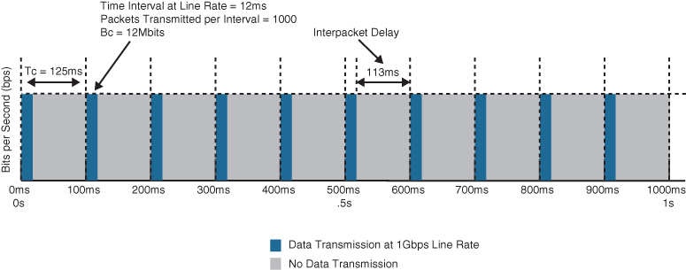
Figure 14-11 Token Bucket Operation
The recommended values for Tc range from 8 ms to 125 ms. Shorter Tcs, such as 8 ms to 10 ms, are necessary to reduce interpacket delay for real-time traffic such as voice. Tcs longer than 125 ms are not recommended for most networks because the interpacket delay becomes too large.
Types of Policers
There are different policing algorithms, including the following:
Single-rate two-color marker/policer
Single-rate three-color marker/policer (srTCM)
Two-rate three-color marker/policer (trTCM)
Single-Rate Two-Color Markers/Policers
The first policers implemented use a single-rate, two-color model based on the single token bucket algorithm. For this type of policer, traffic can be either conforming to or exceeding the CIR. Marking down or dropping actions can be performed for each of the two states.
Figure 14-12 illustrates different actions that the single-rate two-color policer can take. The section above the dotted line on the left side of the figure represents traffic that exceeded the CIR and was marked down. The section above the dotted line on the right side of the figure represents traffic that exceeded the CIR and was dropped.
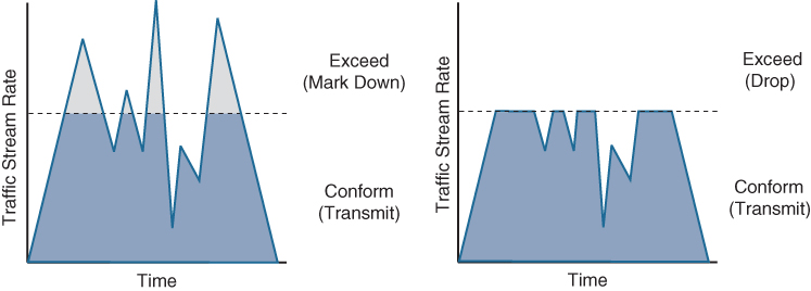
Figure 14-12 Single-Rate Two-Color Marker/Policer
Single-Rate Three-Color Markers/Policers (srTCM)
Single-rate three-color policer algorithms are based on RFC 2697. This type of policer uses two token buckets, and the traffic can be classified as either conforming to, exceeding, or violating the CIR. Marking down or dropping actions are performed for each of the three states of traffic.
The first token bucket operates very similarly to the single-rate two-color system; the difference is that if there are any tokens left over in the bucket after each time period due to low or no activity, instead of discarding the excess tokens (overflow), the algorithm places them in a second bucket to be used later for temporary bursts that might exceed the CIR. Tokens placed in this second bucket are referred to as the excess burst (Be), and Be is the maximum number of bits that can exceed the Bc burst size.
With the two token-bucket mechanism, traffic can be classified in three colors or states, as follows:
Conform: Traffic under Bc is classified as conforming and green. Conforming traffic is usually transmitted and can be optionally re-marked.
Exceed: Traffic over Bc but under Be is classified as exceeding and yellow. Exceeding traffic can be dropped or marked down and transmitted.
Violate: Traffic over Be is classified as violating and red. This type of traffic is usually dropped but can be optionally marked down and transmitted.
Figure 14-13 illustrates different actions that a single-rate three-color policer can take. The section below the straight dotted line on the left side of the figure represents the traffic that conformed to the CIR, the section right above the straight dotted line represents the exceeding traffic that was marked down, and the top section represents the violating traffic that was also marked down. The exceeding and violating traffic rates vary because they rely on random tokens spilling over from the Bc bucket into the Be. The section right above the straight dotted line on the right side of the figure represents traffic that exceeded the CIR and was marked down and the top section represents traffic that violated the CIR and was dropped.
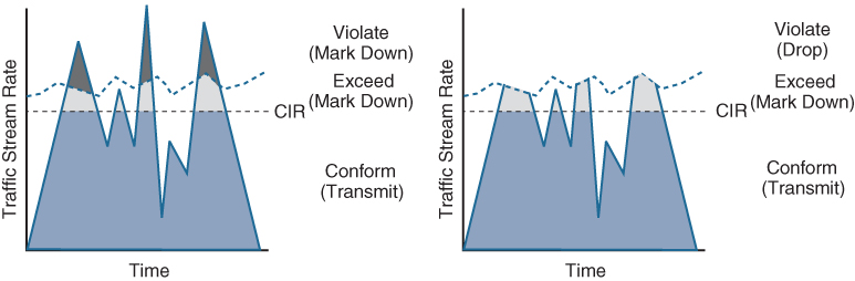
Figure 14-13 Single-Rate Three-Color Marker/Policer
The single-rate three-color marker/policer uses the following parameters to meter the traffic stream:
Committed Information Rate (CIR): The policed rate.
Committed Burst Size (Bc): The maximum size of the CIR token bucket, measured in bytes. Referred to as Committed Burst Size (CBS) in RFC 2697.
Excess Burst Size (Be): The maximum size of the excess token bucket, measured in bytes. Referred to as Excess Burst Size (EBS) in RFC 2697.
Bc Bucket Token Count (Tc): The number of tokens in the Bc bucket. Not to be confused with the committed time interval Tc.
Be Bucket Token Count (Te): The number of tokens in the Be bucket.
Incoming Packet Length (B): The packet length of the incoming packet, in bits.
Figure 14-14 illustrates the logical flow of the single-rate three-color marker/policer two-token-bucket algorithm.
The single-rate three-color policer’s two bucket algorithm causes fewer TCP retransmissions and is more efficient for bandwidth utilization. It is the perfect policer to be used with AF classes (AFx1, AFx2, and AFx3). Using a three-color policer makes sense only if the actions taken for each color differ. If the actions for two or more colors are the same, for example, conform and exceed both transmit without re-marking, the single-rate two-color policer is recommended to keep things simpler.

Figure 14-14 Single-Rate Three-Color Marker/Policer Token Bucket Algorithm
Two-Rate Three-Color Markers/Policers (trTCM)
The two-rate three-color marker/policer is based on RFC 2698 and is similar to the single-rate three-color policer. The difference is that single-rate three-color policers rely on excess tokens from the Bc bucket, which introduces a certain level of variability and unpredictability in traffic flows; the two-rate three-color marker/policers address this issue by using two distinct rates, the CIR and the Peak Information Rate (PIR). The two-rate three-color marker/policer allows for a sustained excess rate based on the PIR that allows for different actions for the traffic exceeding the different burst values; for example, violating traffic can be dropped at a defined rate, and this is something that is not possible with the single-rate three-color policer. Figure 14-15 illustrates how violating traffic that exceeds the PIR can either be marked down (on the left side of the figure) or dropped (on the right side of the figure). Compare Figure 14-15 to Figure 14-14 to see the difference between the two-rate three-color policer and the single-rate three-color policer.
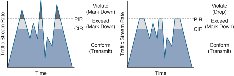
Figure 14-15 Two-Rate Three-Color Marker/Policer Token Bucket Algorithm
The two-rate three-color marker/policer uses the following parameters to meter the traffic stream:
Committed Information Rate (CIR): The policed rate.
Peak Information Rate (PIR): The maximum rate of traffic allowed. PIR should be equal to or greater than the CIR.
Committed Burst Size (Bc): The maximum size of the second token bucket, measured in bytes. Referred to as Committed Burst Size (CBS) in RFC 2698.
Peak Burst Size (Be): The maximum size of the PIR token bucket, measured in bytes. Referred to as Peak Burst Size (PBS) in RFC 2698. Be should be equal to or greater than Bc.
Bc Bucket Token Count (Tc): The number of tokens in the Bc bucket. Not to be confused with the committed time interval Tc.
Bp Bucket Token Count (Tp): The number of tokens in the Bp bucket.
Incoming Packet Length (B): The packet length of the incoming packet, in bits.
The two-rate three-color policer also uses two token buckets, but the logic varies from that of the single-rate three-color policer. Instead of transferring unused tokens from the Bc bucket to the Be bucket, this policer has two separate buckets that are filled with two separate token rates. The Be bucket is filled with the PIR tokens, and the Bc bucket is filled with the CIR tokens. In this model, the Be represents the peak limit of traffic that can be sent during a subsecond interval.
The logic varies further in that the initial check is to see whether the traffic is within the PIR. Only then is the traffic compared against the CIR. In other words, a violate condition is checked first, then an exceed condition, and finally a conform condition, which is the reverse of the logic of the single-rate three-color policer. Figure 14-16 illustrates the token bucket algorithm for the two-rate three-color marker/policer. Compare it to the token bucket algorithm of the single-rate three-color marker/policer in Figure 14-14 to see the differences between the two.
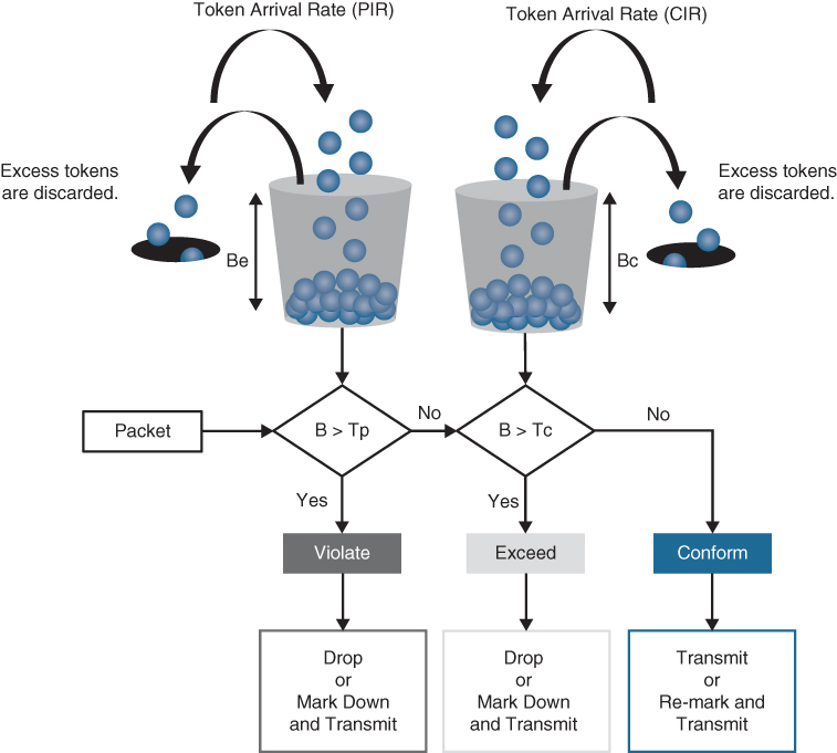
Figure 14-16 Two-Rate Three-Color Marker/Policer Token Bucket Algorithm
Congestion Management and Avoidance
This section explores the queuing algorithms used for congestion management as well as packet drop techniques that can be used for congestion avoidance. These tools provide a way of managing excessive traffic during periods of congestion.
Congestion Management
Congestion management involves a combination of queuing and scheduling. Queuing (also known as buffering) is the temporary storage of excess packets. Queuing is activated when an output interface is experiencing congestion and deactivated when congestion clears. Congestion is detected by the queuing algorithm when a Layer 1 hardware queue present on physical interfaces, known as the transmit ring (Tx-ring or TxQ), is full. When the Tx-ring is not full anymore, this indicates that there is no congestion on the interface, and queueing is deactivated. Congestion can occur for one of these two reasons:
The input interface is faster than the output interface.
The output interface is receiving packets from multiple input interfaces.
When congestion is taking place, the queues fill up, and packets can be reordered by some of the queuing algorithms so that higher-priority packets exit the output interface sooner than lower-priority ones. At this point, a scheduling algorithm decides which packet to transmit next. Scheduling is always active, regardless of whether the interface is experiencing congestion.
There are many queuing algorithms available, but most of them are not adequate for modern rich-media networks carrying voice and high-definition video traffic because they were designed before these traffic types came to be. The legacy queuing algorithms that predate the MQC architecture include the following:
First-in, first-out queuing (FIFO): FIFO involves a single queue where the first packet to be placed on the output interface queue is the first packet to leave the interface (first come, first served). In FIFO queuing, all traffic belongs to the same class.
Round robin: With round robin, queues are serviced in sequence one after the other, and each queue processes one packet only. No queues starve with round robin because every queue gets an opportunity to send one packet every round. No queue has priority over others, and if the packet sizes from all queues are about the same, the interface bandwidth is shared equally across the round robin queues. A limitation of round robin is it does not include a mechanism to prioritize traffic.
Weighted round robin (WRR): WRR was developed to provide prioritization capabilities for round robin. It allows a weight to be assigned to each queue, and based on that weight, each queue effectively receives a portion of the interface bandwidth that is not necessarily equal to the other queues’ portions.
Custom queuing (CQ): CQ is a Cisco implementation of WRR that involves a set of 16 queues with a round-robin scheduler and FIFO queueing within each queue. Each queue can be customized with a portion of the link bandwidth for each selected traffic type. If a particular type of traffic is not using the bandwidth reserved for it, other traffic types may use the unused bandwidth. CQ causes long delays and also suffers from all the same problems as FIFO within each of the 16 queues that it uses for traffic classification.
Priority queuing (PQ): With PQ, a set of four queues (high, medium, normal, and low) are served in strict-priority order, with FIFO queueing within each queue. The high-priority queue is always serviced first, and lower-priority queues are serviced only when all higher-priority queues are empty. For example, the medium queue is serviced only when the high-priority queue is empty. The normal queue is serviced only when the high and medium queues are empty; finally, the low queue is serviced only when all the other queues are empty. At any point in time, if a packet arrives for a higher queue, the packet from the higher queue is processed before any packets in lower-level queues. For this reason, if the higher-priority queues are continuously being serviced, the lower-priority queues are starved.
Weighted fair queuing (WFQ): The WFQ algorithm automatically divides the interface bandwidth by the number of flows (weighted by IP Precedence) to allocate bandwidth fairly among all flows. This method provides better service for high-priority real-time flows but can’t provide a fixed-bandwidth guarantee for any particular flow.
The current queuing algorithms recommended for rich-media networks (and supported by MQC) combine the best features of the legacy algorithms. These algorithms provide real-time, delay-sensitive traffic bandwidth and delay guarantees while not starving other types of traffic. The recommended queuing algorithms include the following:
Class-based weighted fair queuing (CBWFQ): CBWFQ enables the creation of up to 256 queues, serving up to 256 traffic classes. Each queue is serviced based on the bandwidth assigned to that class. It extends WFQ functionality to provide support for user-defined traffic classes. With CBWFQ, packet classification is done based on traffic descriptors such as QoS markings, protocols, ACLs, and input interfaces. After a packet is classified as belonging to a specific class, it is possible to assign bandwidth, weight, queue limit, and maximum packet limit to it. The bandwidth assigned to a class is the minimum bandwidth delivered to the class during congestion. The queue limit for that class is the maximum number of packets allowed to be buffered in the class queue. After a queue has reached the configured queue limit, excess packets are dropped. CBWFQ by itself does not provide a latency guarantee and is only suitable for non-real-time data traffic.
Low-latency queuing (LLQ): LLQ is CBWFQ combined with priority queueing (PQ) and it was developed to meet the requirements of real-time traffic, such as voice. Traffic assigned to the strict-priority queue is serviced up to its assigned bandwidth before other CBWFQ queues are serviced. All real-time traffic should be configured to be serviced by the priority queue. Multiple classes of real-time traffic can be defined, and separate bandwidth guarantees can be given to each, but a single priority queue schedules all the combined traffic. If a traffic class is not using the bandwidth assigned to it, it is shared among the other classes. This algorithm is suitable for combinations of real-time and non-real-time traffic. It provides both latency and bandwidth guarantees to high-priority real-time traffic. In the event of congestion, real-time traffic that goes beyond the assigned bandwidth guarantee is policed by a congestion-aware policer to ensure that the non-priority traffic is not starved.
Figure 14-17 illustrates the architecture of CBWFQ in combination with LLQ.
CBWFQ in combination with LLQ create queues into which traffic classes are classified. The CBWFQ queues are scheduled with a CBWFQ scheduler that guarantees bandwidth to each class. LLQ creates a high-priority queue that is always serviced first. During times of congestion, LLQ priority classes are policed to prevent the PQ from starving the CBWFQ non-priority classes (as legacy PQ does). When LLQ is configured, the policing rate must be specified as either a fixed amount of bandwidth or as a percentage of the interface bandwidth.
LLQ allows for two different traffic classes to be assigned to it so that different policing rates can be applied to different types of high-priority traffic. For example, voice traffic could be policed during times of congestion to 10 Mbps, while video could be policed to 100 Mbps. This would not be possible with only one traffic class and a single policer.
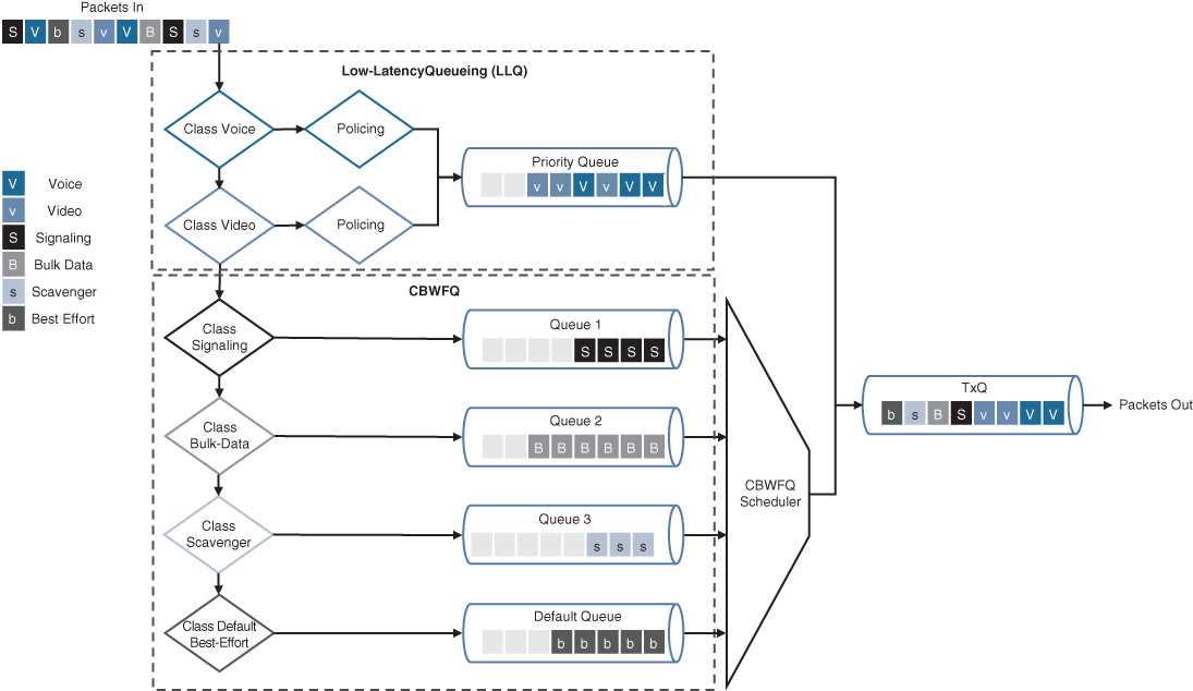
Figure 14-17 CBWFQ with LLQ
Congestion-Avoidance Tools
Congestion-avoidance techniques monitor network traffic loads to anticipate and avoid congestion by dropping packets. The default packet dropping mechanism is tail drop. Tail drop treats all traffic equally and does not differentiate between classes of service. With tail drop, when the output queue buffers are full, all packets trying to enter the queue are dropped, regardless of their priority, until congestion clears up and the queue is no longer full. Tail drop should be avoided for TCP traffic because it can cause TCP global synchronization, which results in significant link underutilization.
A better approach is to use a mechanism known as random early detection (RED). RED provides congestion avoidance by randomly dropping packets before the queue buffers are full. Randomly dropping packets instead of dropping them all at once, as with tail drop, avoids global synchronization of TCP streams. RED monitors the buffer depth and performs early drops on random packets when the minimum defined queue threshold is exceeded.
The Cisco implementation of RED is known as weighted RED (WRED). The difference between RED and WRED is that the randomness of packet drops can be manipulated by traffic weights denoted by either IP Precedence (IPP) or DSCP. Packets with a lower IPP value are dropped more aggressively than are higher IPP values; for example, IPP 3 would be dropped more aggressively than IPP 5 or DSCP, AFx3 would be dropped more aggressively than AFx2, and AFx2 would be dropped more aggressively than AFx1.
WRED can also be used to set the IP Explicit Congestion Notification (ECN) bits to indicate that congestion was experienced in transit. ECN is an extension to WRED that allows for signaling to be sent to ECN-enabled endpoints, instructing them to reduce their packet transmission rates.
Exam Preparation Tasks
As mentioned in the section “How to Use This Book” in the Introduction, you have a couple of choices for exam preparation: the exercises here, Chapter 30, “Final Preparation,” and the exam simulation questions in the Pearson Test Prep Software Online.
Review All Key Topics
Review the most important topics in the chapter, noted with the key topics icon in the outer margin of the page. Table 14-6 lists these key topics and the page number on which each is found.
Table 14-6 Key Topics for Chapter 14
Key Topic Element |
Description |
Page |
List |
QoS models |
|
Paragraph |
Integrated Services (IntServ) |
|
Paragraph |
Differentiated Services (DiffServ) |
|
Section |
Classification |
|
List |
Classification traffic descriptors |
|
Paragraph |
Next Generation Network Based Application Recognition (NBAR2) |
|
Section |
Marking |
|
List |
Marking traffic descriptors |
|
Paragraph |
802.1Q/p |
|
List |
802.1Q Tag Control Information (TCI) field |
|
Section |
Priority Code Point (PCP) field |
|
Paragraph |
Type of Service (ToS) field |
|
Paragraph |
Differentiated Services Code Point (DSCP) field |
|
Paragraph |
Per-hop behavior (PHB) definition |
|
List |
Available PHBs |
|
Section |
Trust boundary |
|
Paragraph |
Policing and shaping definition |
|
Section |
Markdown |
|
List |
Token bucket algorithm key definitions |
|
List |
Policing algorithms |
|
List |
Legacy queuing algorithms |
|
List |
Current queuing algorithms |
|
Paragraph |
Weighted random early detection (WRED) |
Complete Tables and Lists from Memory
Print a copy of Appendix B, “Memory Tables” (found on the companion website), or at least the section for this chapter, and complete the tables and lists from memory. Appendix C, “Memory Tables Answer Key,” also on the companion website, includes completed tables and lists you can use to check your work.
Define Key Terms
Define the following key terms from this chapter and check your answers in the Glossary:
Differentiated Services (DiffServ)
References In This Chapter
RFC 1633, Integrated Services in the Internet Architecture: an Overview, R. Braden, D. Clark, S. Shenker. https://tools.ietf.org/html/rfc1633, June 1994
RFC 2474, Definition of the Differentiated Services Field (DS Field) in the IPv4 and IPv6 Headers, K. Nichols, S. Blake, F. Baker, D. Black. https://tools.ietf.org/html/rfc2474, December 1998
RFC 2475, An Architecture for Differentiated Services, S. Blake, D. Black, M. Carlson, E. Davies, Z. Wang, W. Weiss. https://tools.ietf.org/html/rfc2475, December 1998
RFC 2597, Assured Forwarding PHB Group, J. Heinanen, Telia Finland, F. Baker, W. Weiss, J. Wroclawski. https://tools.ietf.org/html/rfc2597, June 1999
RFC 2697, A Single Rate Three Color Marker, J. Heinanen, Telia Finland, R. Guerin, IETF. https://tools.ietf.org/html/rfc2697, September 1999
RFC 2698, A Two Rate Three Color Marker, J. Heinanen, Telia Finland, R. Guerin, IETF. https://tools.ietf.org/html/rfc2698, September 1999
RFC 3140, Per Hop Behavior Identification Codes, D. Black, S. Brim, B. Carpenter,F. Le Faucheur, IETF. https://tools.ietf.org/html/rfc3140, June 2001
RFC 3246, An Expedited Forwarding PHB (Per-Hop Behavior), B. Davie, A. Charny, J.C.R. Bennett, K. Benson, J.Y. Le Boudec, W. Courtney, S. Davari, V. Firoiu,D. Stiliadis. https://tools.ietf.org/html/rfc3246, March 2002
RFC 3260, New Terminology and Clarifications for Diffserv, D. Grossman, IETF. https://tools.ietf.org/html/rfc3260, April 2002
RFC 3594, Configuration Guidelines for DiffServ Service Classes, J. Babiarz, K. Chan, F. Baker, IETF. https://tools.ietf.org/html/rfc4594, August 2006
draft-suznjevic-tsvwg-delay-limits-00, Delay Limits for Real-Time Services, M. Suznjevic, J. Saldana, IETF. https://tools.ietf.org/html/draft-suznjevic-tsvwg-delay-limits-00, June 2016