
Chapter 17. Wireless Signals and Modulation
This chapter covers the following subjects:
Understanding Basic Wireless Theory: This section covers the basic theory behind radio frequency (RF) signals, as well as measuring and comparing the power of RF signals.
Carrying Data over a Wireless Signal: This section provides an overview of basic methods and standards that are involved in carrying data wirelessly between devices and the network.
Wireless LANs must transmit a signal over radio frequencies to move data from one device to another. Transmitters and receivers can be fixed in consistent locations, or they can be free to move around. This chapter covers the basic theory behind wireless signals and the methods used to carry data wirelessly.
“Do I Know This Already?” Quiz
The “Do I Know This Already?” quiz allows you to assess whether you should read the entire chapter. If you miss no more than one of these self-assessment questions, you might want to move ahead to the “Exam Preparation Tasks” section. Table 17-1 lists the major headings in this chapter and the “Do I Know This Already?” quiz questions covering the material in those headings so you can assess your knowledge of these specific areas. The answers to the “Do I Know This Already?” quiz appear in Appendix A, “Answers to the ‘Do I Know This Already?’ Quiz Questions.”
Table 17-1 “Do I Know This Already?” Section-to-Question Mapping
Foundation Topics Section |
Questions |
Understanding Basic Wireless Theory |
1–8 |
Carrying Data Over an RF Signal |
9–10 |
1. Two transmitters are each operating with a transmit power level of 100 mW. When you compare the two absolute power levels, what is the difference in dB?
0 dB
20 dB
100 dB
You can’t compare power levels in dB.
2. A transmitter is configured to use a power level of 17 mW. One day it is reconfigured to transmit at a new power level of 34 mW. How much has the power level increased, in dB?
0 dB
2 dB
3 dB
17 dB
None of these answers are correct; you need a calculator to figure this out.
3. Transmitter A has a power level of 1 mW, and transmitter B is 100 mW. Compare transmitter B to A using dB, and then identify the correct answer from the following choices.
0 dB
1 dB
10 dB
20 dB
100 dB
4. A transmitter normally uses an absolute power level of 100 mW. Through the course of needed changes, its power level is reduced to 40 mW. What is the power-level change in dB?
2.5 dB
4 dB
−4 dB
−40 dB
None of these answers are correct; where is that calculator?
5. Consider a scenario with a transmitter and a receiver that are separated by some distance. The transmitter uses an absolute power level of 20 dBm. A cable connects the transmitter to its antenna. The receiver also has a cable connecting it to its antenna. Each cable has a loss of 2 dB. The transmitting and receiving antennas each have a gain of 5 dBi. What is the resulting EIRP?
+20 dBm
+23 dBm
+26 dBm
+34 dBm
None of these answers are correct.
6. A receiver picks up an RF signal from a distant transmitter. Which one of the following represents the best signal quality received? Example values are given in parentheses.
Low SNR (10 dB), low RSSI (−75 dBm)
High SNR (30 dB), low RSSI (−75 dBm)
Low SNR (10 dB), high RSSI (−55 dBm)
High SNR (30 dB), high RSSI (−55 dBm)
7. Which one of the following is the primary cause of free space path loss?
Spreading
Absorption
Humidity levels
Magnetic field decay
8. Which one of the following has the shortest effective range in free space, assuming that the same transmit power level is used for each?
An 802.11g device
An 802.11a device
An 802.11b device
None of these answers
9. QAM alters which of the following aspects of an RF signal? (Choose two.)
Frequency
Amplitude
Phase
Quadrature
10. Suppose that an 802.11a device moves away from a transmitter. As the signal strength decreases, which one of the following might the device or the transmitter do to improve the signal quality along the way?
Aggregate more channels
Use more radio chains
Switch to a more complex modulation scheme
Switch to a less complex modulation scheme
Answers to the “Do I Know This Already?” quiz:
1 A
2 C
3 D
4 C
5 B
6 D
7 A
8 B
9 B, C
10 D
Foundation Topics
Understanding Basic Wireless Theory
To send data across a wired link, an electrical signal is applied at one end and is carried to the other end. The wire itself is continuous and conductive, so the signal can propagate rather easily. A wireless link has no physical strands of anything to carry the signal along.
How then can an electrical signal be sent across the air, or free space? Consider a simple analogy of two people standing far apart, and one person wants to signal something to the other. They are connected by a long and somewhat-loose rope; the rope represents free space. The sender at one end decides to lift his end of the rope high and hold it there so that the other end of the rope will also raise and notify the partner. After all, if the rope were a wire, he knows that he could apply a steady voltage at one end of the wire and it would appear at the other end. Figure 17-1 shows the end result; the rope falls back down after a tiny distance, and the receiver never notices a change at all.
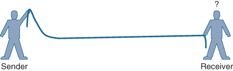
Figure 17-1 Failed Attempt to Pass a Message Down a Rope
The sender decides to try a different strategy. He cannot push the rope toward the receiver, but when he begins to wave it up and down in a steady, regular motion, a curious thing happens. A continuous wave pattern appears along the entire length of the rope, as shown in Figure 17-2. In fact, the waves (each representing one up and down cycle of the sender’s arm) actually travel from the sender to the receiver.

Figure 17-2 Sending a Continuous Wave Down a Rope
In free space, a similar principle occurs. The sender (a transmitter) can send an alternating current into a section of wire (an antenna), which sets up moving electric and magnetic fields that propagate out and away from the wire as traveling waves. The electric and magnetic fields travel along together and are always at right angles to each other, as shown in Figure 17-3. The signal must keep changing, or alternating, by cycling up and down, to keep the electric and magnetic fields cycling and pushing ever outward.

Figure 17-3 Traveling Electric and Magnetic Waves
Electromagnetic waves do not travel strictly in a straight line. Instead, they travel by expanding in all directions away from the antenna. To get a visual image, think of dropping a pebble into a pond when the surface is still. Where it drops in, the pebble sets the water’s surface into a cyclic motion. The waves that result begin small and expand outward, only to be replaced by new waves. In free space, the electromagnetic waves expand outward in all three dimensions.
Figure 17-4 shows a simple idealistic antenna that is a single point, which is connected at the end of a wire. The waves produced from the tiny point antenna expand outward in a spherical shape. The waves will eventually reach the receiver, in addition to many other locations in other directions.
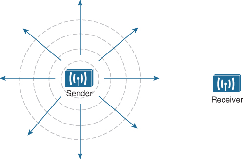
Figure 17-4 Wave Propagation with an Idealistic Antenna
At the receiving end of a wireless link, the process is reversed. As the electromagnetic waves reach the receiver’s antenna, they induce an electrical signal. If everything works right, the received signal will be a reasonable copy of the original transmitted signal.
Understanding Frequency
The waves involved in a wireless link can be measured and described in several ways. One fundamental property is the frequency of the wave, or the number of times the signal makes one complete up and down cycle in 1 second. Figure 17-5 shows how a cycle of a wave can be identified. A cycle can begin as the signal rises from the center line, falls through the center line, and rises again to meet the center line. A cycle can also be measured from the center of one peak to the center of the next peak. No matter where you start measuring a cycle, the signal must make a complete sequence back to its starting position where it is ready to repeat the same cyclic pattern again.

Figure 17-5 Cycles Within a Wave
In Figure 17-5, suppose that 1 second has elapsed, as shown. During that 1 second, the signal progressed through four complete cycles. Therefore, its frequency is 4 cycles/second, or 4 hertz. A hertz (Hz) is the most commonly used frequency unit and is nothing other than one cycle per second.
Frequency can vary over a very wide range. As frequency increases by orders of magnitude, the numbers can become quite large. To keep things simple, the frequency unit name can be modified to denote an increasing number of zeros, as listed in Table 17-2.
Table 17-2 Frequency Unit Names
Unit |
Abbreviation |
Meaning |
Hertz |
Hz |
Cycles per second |
Kilohertz |
kHz |
1000 Hz |
Megahertz |
MHz |
1,000,000 Hz |
Gigahertz |
GHz |
1,000,000,000 Hz |
Figure 17-6 shows a simple representation of the continuous frequency spectrum ranging from 0 Hz to 1022 (or 1 followed by 22 zeros) Hz. At the low end of the spectrum are frequencies that are too low to be heard by the human ear, followed by audible sounds. The highest range of frequencies contains light, followed by X, gamma, and cosmic rays.
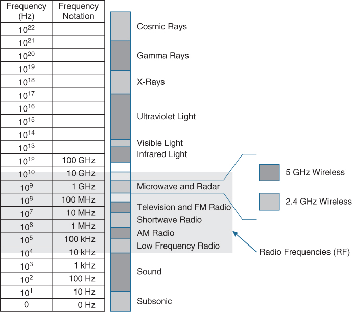
Figure 17-6 Continuous Frequency Spectrum
The frequency range from around 3 kHz to 300 GHz is commonly called radio frequency (RF). It includes many different types of radio communication, such as low-frequency radio, AM radio, shortwave radio, television, FM radio, microwave, and radar. The microwave category also contains the two main frequency ranges that are used for wireless LAN communication: 2.4 and 5 GHz.
Because a range of frequencies might be used for the same purpose, it is customary to refer to the range as a band of frequencies. For example, the range from 530 kHz to around 1710 kHz is used by AM radio stations; therefore it is commonly called the AM band or the AM broadcast band.
One of the two main frequency ranges used for wireless LAN communication lies between 2.400 and 2.4835 GHz. This is usually called the 2.4 GHz band, even though it does not encompass the entire range between 2.4 and 2.5 GHz. It is much more convenient to refer to the band name instead of the specific range of frequencies included.
The other wireless LAN range is usually called the 5 GHz band because it lies between 5.150 and 5.825 GHz. The 5 GHz band actually contains the following four separate and distinct bands:
5.150 to 5.250 GHz
5.250 to 5.350 GHz
5.470 to 5.725 GHz
5.725 to 5.825 GHz
It is interesting that the 5 GHz band can contain several smaller bands. Remember that the term band is simply a relative term that is used for convenience.
A frequency band contains a continuous range of frequencies. If two devices require a single frequency for a wireless link between them, which frequency can they use? Beyond that, how many unique frequencies can be used within a band?
To keep everything orderly and compatible, bands are usually divided up into a number of distinct channels. Each channel is known by a channel number and is assigned to a specific frequency. As long as the channels are defined by a national or international standards body, they can be used consistently in all locations.
For example, Figure 17-7 shows the channel assignment for the 2.4 GHz band that is used for wireless LAN communication. The band contains 14 channels numbered 1 through 14, each assigned a specific frequency. First, notice how much easier it is to refer to channel numbers than the frequencies. Second, notice that the channels are spaced at regular intervals that are 0.005 GHz (or 5 MHz) apart, except for channel 14. The channel spacing is known as the channel separation or channel width.

Figure 17-7 Example of Channel Spacing in the 2.4 GHz Band
If devices use a specific frequency for a wireless link, why do the channels need to be spaced apart at all? The reason lies with the practical limitations of RF signals, the electronics involved in transmitting and receiving the signals, and the overhead needed to add data to the signal effectively.
In practice, an RF signal is not infinitely narrow; instead, it spills above and below a center frequency to some extent, occupying neighboring frequencies, too. It is the center frequency that defines the channel location within the band. The actual frequency range needed for the transmitted signal is known as the signal bandwidth, as shown in Figure 17-8. As its name implies, bandwidth refers to the width of frequency space required within the band. For example, a signal with a 22 MHz bandwidth is bounded at 11 MHz above and below the center frequency. In wireless LANs, the signal bandwidth is defined as part of a standard. Even though the signal might extend farther above and below the center frequency than the bandwidth allows, wireless devices will use something called a spectral mask to ignore parts of the signal that fall outside the bandwidth boundaries.

Figure 17-8 Signal Bandwidth
Ideally, the signal bandwidth should be less than the channel width so that a different signal could be transmitted on every possible channel, with no chance that two signals could overlap and interfere with each other. Figure 17-9 shows such a channel spacing, where the signals on adjacent channels do not overlap. A signal can exist on every possible channel without overlapping with others.

Figure 17-9 Non-overlapping Channel Spacing
However, you should not assume that signals centered on the standardized channel assignments will not overlap with each other. It is entirely possible that the channels in a band are narrower than the signal bandwidth, as shown in Figure 17-10. Notice how two signals have been centered on adjacent channel numbers 1 and 2, but they almost entirely overlap each other! The problem is that the signal bandwidth is slightly wider than four channels. In this case, signals centered on adjacent channels cannot possibly coexist without overlapping and interfering. Instead, the signals must be placed on more distant channels to prevent overlapping, thus limiting the number of channels that can be used in the band.
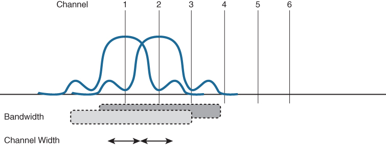
Figure 17-10 Overlapping Channel Spacing
Understanding Phase
RF signals are very dependent upon timing because they are always in motion. By their very nature, the signals are made up of electrical and magnetic forces that vary over time. The phase of a signal is a measure of shift in time relative to the start of a cycle. Phase is normally measured in degrees, where 0 degrees is at the start of a cycle, and one complete cycle equals 360 degrees. A point that is halfway along the cycle is at the 180-degree mark. Because an oscillating signal is cyclic, you can think of the phase traveling around a circle again and again.
When two identical signals are produced at exactly the same time, their cycles match up and they are said to be in phase with each other. If one signal is delayed from the other, the two signals are said to be out of phase. Figure 17-11 shows examples of both scenarios.

Figure 17-11 Signals In and Out of Phase
Phase becomes important as RF signals are received. Signals that are in phase tend to add together, whereas signals that are 180 degrees out of phase tend to cancel each other out.
Measuring Wavelength
RF signals are usually described by their frequency; however, it is difficult to get a feel for their physical size as they move through free space. The wavelength is a measure of the physical distance that a wave travels over one complete cycle. Wavelength is usually designated by the Greek symbol lambda (λ). To get a feel for the dimensions of a wireless LAN signal, assuming that you could see it as it travels in front of you, a 2.4 GHz signal would have a wavelength of 4.92 inches, while a 5 GHz signal would be 2.36 inches.
Figure 17-12 shows the wavelengths of three different waves. The waves are arranged in order of increasing frequency, from top to bottom. Regardless of the frequency, RF waves travel at a constant speed. In a vacuum, radio waves travel at exactly the speed of light; in air, the velocity is slightly less than the speed of light. Notice that the wavelength decreases as the frequency increases. As the wave cycles get smaller, they cover less distance. Wavelength becomes useful in the design and placement of antennas.

Figure 17-12 Examples of Increasing Frequency and Decreasing Wavelength
Understanding RF Power and dB
For an RF signal to be transmitted, propagated through free space, received, and understood with any certainty, it must be sent with enough strength or energy to make the journey. Think about Figure 17-1 again, where the two people are trying to signal each other with a rope. If the sender continuously moves his arm up and down a small distance, he will produce a wave in the rope. However, the wave will dampen out only a short distance away because of factors such as the weight of the rope, gravity, and so on. To move the wave all the way down the rope to reach the receiver, the sender must move his arm up and down with a much greater range of motion and with greater force or strength.
This strength can be measured as the amplitude, or the height from the top peak to the bottom peak of the signal’s waveform, as shown in Figure 17-13.

Figure 17-13 Signal Amplitude
The strength of an RF signal is usually measured by its power, in watts (W). For example, a typical AM radio station broadcasts at a power of 50,000 W; an FM radio station might use 16,000 W. In comparison, a wireless LAN transmitter usually has a signal strength between 0.1 W (100 mW) and 0.001 W (1 mW).
When power is measured in watts or milliwatts, it is considered to be an absolute power measurement. In other words, something has to measure exactly how much energy is present in the RF signal. This is fairly straightforward when the measurement is taken at the output of a transmitter because the transmit power level is usually known ahead of time.
Sometimes you might need to compare the power levels between two different transmitters. For example, suppose that device T1 is transmitting at 1 mW, while T2 is transmitting at 10 mW, as shown in Figure 17-14. Simple subtraction tells you that T2 is 9 mW stronger than T1. You might also notice that T2 is 10 times stronger than T1.

Figure 17-14 Comparing Power Levels Between Transmitters
Now compare transmitters T2 and T3, which use 10 mW and 100 mW, respectively. Using subtraction, T2 and T3 differ by 90 mW, but T3 is again 10 times stronger than T2. In each instance, subtraction yields a different result than division. Which method should you use?
Quantities like absolute power values can differ by orders of magnitude. A more surprising example is shown in Figure 17-15, where T4 is 0.00001 mW, and T5 is 10 mW—values you might encounter with wireless access points. Subtracting the two values gives their difference as 9.99999 mW. However, T5 is 1,000,000 times stronger than T4!
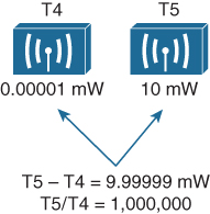
Figure 17-15 Comparing Power Levels That Differ By Orders of Magnitude
Because absolute power values can fall anywhere within a huge range, from a tiny decimal number to hundreds, thousands, or greater values, we need a way to transform the exponential range into a linear one. The logarithm function can be leveraged to do just that. In a nutshell, a logarithm takes values that are orders of magnitude apart (0.001, 0.01, 0.1, 1, 10, 100, and 1000, for example) and spaces them evenly within a reasonable range.
The decibel (dB) is a handy function that uses logarithms to compare one absolute measurement to another. It was originally developed to compare sound intensity levels, but it applies directly to power levels, too. After each power value has been converted to the same logarithmic scale, the two values can be subtracted to find the difference. The following equation is used to calculate a dB value, where P1 and P2 are the absolute power levels of two sources:
P2 represents the source of interest, and P1 is usually called the reference value or the source of comparison.
The difference between the two logarithmic functions can be rewritten as a single logarithm of P2 divided by P1, as follows:
Here, the ratio of the two absolute power values is computed first; then the result is converted onto a logarithmic scale.
Oddly enough, we end up with the same two methods to compare power levels with dB: a subtraction and a division. Thanks to the logarithm, both methods arrive at identical dB values. Be aware that the ratio or division form of the equation is the most commonly used in the wireless engineering world.
Important dB Laws to Remember
There are three cases where you can use mental math to make power-level comparisons using dB. By adding or subtracting fixed dB amounts, you can compare two power levels through multiplication or division. You should memorize the following three laws, which are based on dB changes of 0, 3, and 10, respectively:
Law of Zero: A value of 0 dB means that the two absolute power values are equal.
If the two power values are equal, the ratio inside the logarithm is 1, and the log10(1) is 0. This law is intuitive; if two power levels are the same, one is 0 dB greater than the other.
Law of 3s: A value of 3 dB means that the power value of interest is double the reference value; a value of −3 dB means the power value of interest is half the reference.
When P2 is twice P1, the ratio is always 2. Therefore, 10log10(2) = 3 dB.
When the ratio is 1/2, 10log10(1/2) = −3 dB.
The Law of 3s is not very intuitive, but is still easy to learn. Whenever a power level doubles, it increases by 3 dB. Whenever it is cut in half, it decreases by 3 dB.
Law of 10s: A value of 10 dB means that the power value of interest is 10 times the reference value; a value of −10 dB means the power value of interest is 1/10 of the reference.
When P2 is 10 times P1, the ratio is always 10. Therefore, 10log10(10) = 10 dB.
When P2 is one tenth of P1, then the ratio is 1/10 and 10log10(1/10) = −10 dB.
The Law of 10s is intuitive because multiplying or dividing by 10 adds or subtracts 10 dB, respectively.
Notice another handy rule of thumb: When absolute power values multiply, the dB value is positive and can be added. When the power values divide, the dB value is negative and can be subtracted. Table 17-3 summarizes the useful dB comparisons.
Table 17-3 Power Changes and Their Corresponding dB Values
Power Change |
dB Value |
= |
0 dB |
× 2 |
+3 dB |
/ 2 |
−3 dB |
× 10 |
+10 dB |
/ 10 |
−10 dB |
Try a few example problems to see whether you understand how to compare two power values using dB. In Figure 17-16, sources A, B, and C transmit at 4, 8, and 16 mW, respectively. Source B is double the value of A, so it must be 3 dB greater than A. Likewise, source C is double the value of B, so it must be 3 dB greater than B.
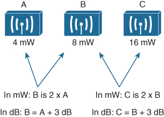
Figure 17-16 Comparing Power Levels Using dB
You can also compare sources A and C. To get from A to C, you have to double A, and then double it again. Each time you double a value, just add 3 dB. Therefore, C is 3 dB + 3 dB = 6 dB greater than A.
Next, try the more complicated example shown in Figure 17-17. Keep in mind that dB values can be added and subtracted in succession (in case several multiplication and division operations involving 2 and 10 are needed).

Figure 17-17 Example of Computing dB with Simple Rules
Sources D and E have power levels 5 and 200 mW. Try to figure out a way to go from 5 to 200 using only × 2 or × 10 operations. You can double 5 to get 10, then double 10 to get 20, and then multiply by 10 to reach 200 mW. Next, use the dB laws to replace the doubling and × 10 with the dB equivalents. The result is E = D + 3 + 3 + 10 or E = D + 16 dB.
You might also find other ways to reach the same result. For example, you can start with 5 mW, then multiply by 10 to get 50, then double 50 to get 100, then double 100 to reach 200 mW. This time the result is E = D + 10 + 3 + 3 or E = D + 16 dB.
Comparing Power Against a Reference: dBm
Beyond comparing two transmitting sources, a network engineer must be concerned about the RF signal propagating from a transmitter to a receiver. After all, transmitting a signal is meaningless unless someone can receive it and make use of that signal.
Figure 17-18 shows a simple scenario with a transmitter and a receiver. Nothing in the real world is ideal, so assume that something along the path of the signal will induce a net loss. At the receiver, the signal strength will be degraded by some amount. Suppose that you are able to measure the power level leaving the transmitter, which is 100 mW. At the receiver, you measure the power level of the arriving signal. It is an incredibly low 0.000031623 mW.
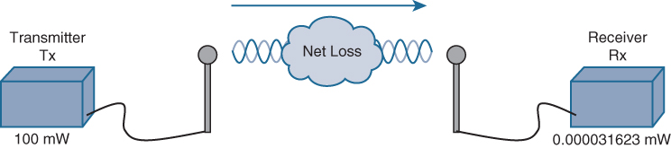
Figure 17-18 Example of RF Signal Power Loss
Wouldn’t it be nice to quantify the net loss over the signal’s path? After all, you might want to try several other transmit power levels or change something about the path between the transmitter and receiver. To design the signal path properly, you would like to make sure that the signal strength arriving at the receiver is at an optimum level.
You could leverage the handy dB formula to compare the received signal strength to the transmitted signal strength, as long as you can remember the formula and have a calculator nearby:
The net loss over the signal path turns out to be a decrease of 65 dB. Knowing that, you decide to try a different transmit power level to see what would happen at the receiver. It does not seem very straightforward to use the new transmit power to find the new signal strength at the receiver. That might require more formulas and more time at the calculator.
A better approach is to compare each absolute power along the signal path to one common reference value. Then, regardless of the absolute power values, you could just focus on the changes to the power values that are occurring at various stages along the signal path. In other words, you could convert every power level to a dB value and simply add them up along the path.
Recall that the dB formula puts the power level of interest on the top of the ratio, with a reference power level on the bottom. In wireless networks, the reference power level is usually 1 mW, so the units are designated by dBm (dB-milliwatt).
Returning to the scenario in Figure 17-18, the absolute power values at the transmitter and receiver can be converted to dBm, the results of which are shown in Figure 17-19. Notice that the dBm values can be added along the path: The transmitter dBm plus the net loss in dB equals the received signal in dBm.
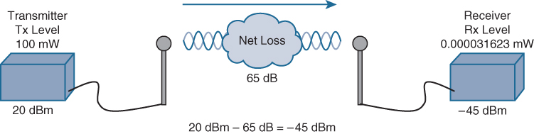
Figure 17-19 Subtracting dB to Represent a Loss in Signal Strength
Measuring Power Changes Along the Signal Path
Up to this point, this chapter has considered a transmitter and its antenna to be a single unit. That might seem like a logical assumption because many wireless access points have built-in antennas. In reality, a transmitter, its antenna, and the cable that connects them are all discrete components that not only propagate an RF signal but also affect its absolute power level.
When an antenna is connected to a transmitter, it provides some amount of gain to the resulting RF signal. This effectively increases the dB value of the signal above that of the transmitter alone. Chapter 18 explains this in greater detail; for now, just be aware that antennas provide positive gain.
By itself, an antenna does not generate any amount of absolute power. In other words, when an antenna is disconnected, no milliwatts of power are being pushed out of it. That makes it impossible to measure the antenna’s gain in dBm. Instead, an antenna’s gain is measured by comparing its performance with that of a reference antenna, then computing a value in dB.
Usually, the reference antenna is an isotropic antenna, so the gain is measured in dBi (dB-isotropic). An isotropic antenna does not actually exist because it is ideal in every way. Its size is a tiny point, and it radiates RF equally in every direction. No physical antenna can do that. The isotropic antenna’s performance can be calculated according to RF formulas, making it a universal reference for any antenna.
Because of the physical qualities of the cable that connects an antenna to a transmitter, some signal loss always occurs. Cable vendors supply the loss in dB per foot or meter of cable length for each type of cable manufactured.
Once you know the complete combination of transmitter power level, the length of cable, and the antenna gain, you can figure out the actual power level that will be radiated from the antenna. This is known as the effective isotropic radiated power (EIRP), measured in dBm.
EIRP is a very important parameter because it is regulated by government agencies in most countries. In those cases, a system cannot radiate signals higher than a maximum allowable EIRP. To find the EIRP of a system, simply add the transmitter power level to the antenna gain and subtract the cable loss, as illustrated in Figure 17-20.
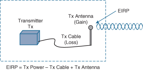
Figure 17-20 Calculating EIRP
Suppose a transmitter is configured for a power level of 10 dBm (10 mW). A cable with 5 dB loss connects the transmitter to an antenna with an 8 dBi gain. The resulting EIRP of the system is 10 dBm – 5 dB + 8 dBi, or 13 dBm.
You might notice that the EIRP is made up of decibel-milliwatt (dBm), dB relative to an isotropic antenna (dBi), and plain decibel (dB) values. Even though the units appear to be different, you can safely combine them for the purposes of calculating the EIRP. The only exception to this is when an antenna’s gain is measured in dBd (dB-dipole). In that case, a dipole antenna has been used as the reference antenna, rather than an isotropic antenna. A dipole is a simple actual antenna, which has a gain of 2.14 dBi. If an antenna has its gain shown as dBi, you can add 2.14 dBi to that value to get its gain in dBi units instead.
Power-level considerations do not have to stop with the EIRP. You should also be concerned with the complete path of a signal, to make sure that the transmitted signal has sufficient power so that it can effectively reach and be understood by a receiver. This is known as the link budget.
The dB values of gains and losses can be combined over any number of stages along a signal’s path. Consider Figure 17-21, which shows every component of signal gain or loss along the path from transmitter to receiver.

Figure 17-21 Calculating Received Signal Strength Over the Path of an RF Signal
At the receiving end, an antenna provides gain to increase the received signal power level. A cable connecting the antenna to the receiver also introduces some loss.
Figure 17-22 shows some example dB values, as well as the resulting sum of the component parts across the entire signal path. The signal begins at 20 dBm at the transmitter, has an EIRP value of 22 dBm at the transmitting antenna (20 dBm − 2 dB + 4 dBi), and arrives at the receiver with a level of −45 dBm.

Figure 17-22 Example of Calculating Received Signal Strength
If you always begin with the transmitter power expressed in dBm, it is a simple matter to add or subtract the dB components along the signal path to find the signal strength that arrives at the receiver.
Free Space Path Loss
Whenever an RF signal is transmitted from an antenna, its amplitude decreases as it travels through free space. Even if there are no obstacles in the path between the transmitter and receiver, the signal strength will weaken. This is known as free space path loss.
What is it about free space that causes an RF signal to be degraded? Is it the air or maybe the earth’s magnetic field? No, even signals sent to and from spacecraft in the vacuum of outer space are degraded.
Recall that an RF signal propagates through free space as a wave, not as a ray or straight line. The wave has a three-dimensional curved shape that expands as it travels. It is this expansion or spreading that causes the signal strength to weaken.
Figure 17-23 shows a cutaway view of the free space loss principle. Suppose the antenna is a tiny point, such that the transmitted RF energy travels in every direction. The wave that is produced would take the form of a sphere; as the wave travels outward, the sphere increases in size. Therefore, the same amount of energy coming out of the tiny point is soon spread over an ever expanding sphere in free space. The concentration of that energy gets weaker as the distance from the antenna increases.
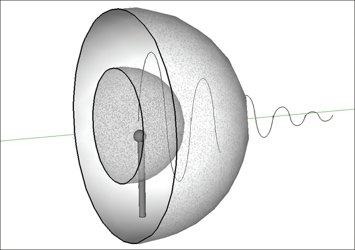
Figure 17-23 Free Space Loss Due to Wave Spreading
Even if you could devise an antenna that could focus the transmitted energy into a tight beam, the energy would still travel as a wave and would spread out over a distance. Regardless of the antenna used, the amount of signal strength loss through free space is consistent.
For reference, the free space path loss (FSPL) in dB can be calculated according to the following equation:
FSPL(dB) = 20log10(d) + 20log10(f) + 32.44
where d is the distance from the transmitter in kilometers and f is the frequency in megahertz. Do not worry, though: You will not have to know this equation for the ENCOR 350-401 exam. It is presented here to show two interesting facts:
Free space path loss is an exponential function; the signal strength falls off quickly near the transmitter but more slowly farther away.
The loss is a function of distance and frequency only.
With the formula, you can calculate the free space path loss for any given scenario, but you will not have to for the exam. Just be aware that the free space path loss is always an important component of the link budget, along with antenna gain and cable loss.
You should also be aware that the free space path loss is greater in the 5 GHz band than it is in the 2.4 GHz band. In the equation, as the frequency increases, so does the loss in dB. This means that 2.4 GHz devices have a greater effective range than 5 GHz devices, assuming an equal transmitted signal strength. Figure 17-24 shows the range difference, where both transmitters have an equal EIRP. The dashed circles show where the effective range ends, at the point where the signal strength of each transmitter is equal.
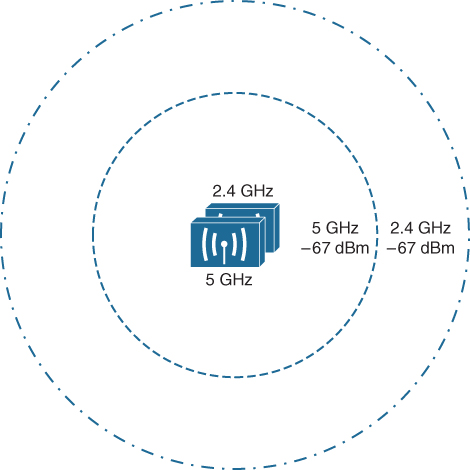
Figure 17-24 Effective Range of 2.4 GHz and 5 GHz Transmitters
Understanding Power Levels at the Receiver
When you work with wireless LAN devices, the EIRP levels leaving the transmitter’s antenna normally range from 100 mW down to 1 mW. This corresponds to the range +20 dBm down to 0 dBm.
At the receiver, the power levels are much, much less, ranging from 1 mW all the way down to tiny fractions of a milliwatt, approaching 0 mW. The corresponding range of received signal levels is from 0 dBm down to about −100 dBm. Even so, a receiver expects to find a signal on a predetermined frequency, with enough power to contain useful data.
Receivers usually measure a signal’s power level according to the received signal strength indicator (RSSI) scale. The RSSI value is defined in the 802.11 standard as an internal 1-byte relative value ranging from 0 to 255, where 0 is the weakest and 255 is the strongest. As such, the value has no useful units and the range of RSSI values can vary between one hardware manufacturer and another. In reality, you will likely see RSSI values that are measured in dBm after they have been converted and scaled to correlate to actual dBm values. Be aware that the results are not standardized across all receiver manufacturers, so an RSSI value can vary from one receiver hardware to another.
Assuming that a transmitter is sending an RF signal with enough power to reach a receiver, what received signal strength value is good enough? Every receiver has a sensitivity level, or a threshold that divides intelligible, useful signals from unintelligible ones. As long as a signal is received with a power level that is greater than the sensitivity level, chances are that the data from the signal can be understood correctly. Figure 17-25 shows an example of how the signal strength at a receiver might change over time. The receiver’s sensitivity level is −82 dBm.

Figure 17-25 Example of Receiver Sensitivity Level
The RSSI value focuses on the expected signal alone, without regard to any other signals that may also be received. All other signals that are received on the same frequency as the one you are trying to receive are simply viewed as noise. The noise level, or the average signal strength of the noise, is called the noise floor.
It is easy to ignore noise as long as the noise floor is well below what you are trying to hear. For example, two people can effectively whisper in a library because there is very little competing noise. Those same two people would become very frustrated if they tried to whisper to each other in a crowded sports arena.
Similarly, with an RF signal, the signal strength must be greater than the noise floor by a decent amount so that it can be received and understood correctly. The difference between the signal and the noise is called the signal-to-noise ratio (SNR), measured in dB. A higher SNR value is preferred.
Figure 17-26 shows the received signal strength of a signal compared with the noise floor that is received. The signal strength averages around −54 dBm. On the left side of the graph, the noise floor is −90 dBm. The resulting SNR is −54 dBm − (−90) dBm or 36 dB. Toward the right side of the graph, the noise floor gradually increases to −65 dBm, reducing the SNR to 11 dB. The signal is so close to the noise that it might not be usable.
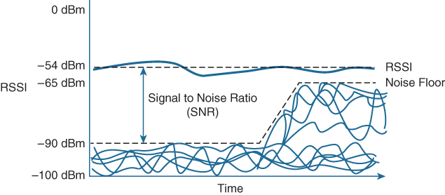
Figure 17-26 Example of a Changing Noise Floor and SNR
Carrying Data Over an RF Signal
Up to this point in the chapter, only the RF characteristics of wireless signals have been discussed. The RF signals presented have existed only as simple oscillations in the form of a sine wave. The frequency, amplitude, and phase have all been constant. The steady, predictable frequency is important because a receiver needs to tune to a known frequency to find the signal in the first place.
This basic RF signal is called a carrier signal because it is used to carry other useful information. With AM and FM radio signals, the carrier signal also transports audio signals. TV carrier signals have to carry both audio and video. Wireless LAN carrier signals must carry data.
To add data to the RF signal, the frequency of the original carrier signal must be preserved. Therefore, there must be some scheme of altering some characteristic of the carrier signal to distinguish a 0 bit from a 1 bit. Whatever scheme is used by the transmitter must also be used by the receiver so that the data bits can be correctly interpreted.
Figure 17-27 shows a carrier signal that has a constant frequency. The data bits 1001 are to be sent over the carrier signal, but how? One idea might be to simply use the value of each data bit to turn the carrier signal off or on. The Bad Idea 1 plot shows the resulting RF signal. A receiver might be able to notice when the signal is present and has an amplitude, thereby correctly interpreting 1 bits, but there is no signal to receive during 0 bits. If the signal becomes weak or is not available for some reason, the receiver will incorrectly think that a long string of 0 bits has been transmitted. A different twist might be to transmit only the upper half of the carrier signal during a 1 bit and the lower half during a 0 bit, as shown in the Bad Idea 2 plot. This time, a portion of the signal is always available for the receiver, but the signal becomes impractical to receive because important pieces of each cycle are missing. In addition, it is very difficult to transmit an RF signal with disjointed alternating cycles.

Figure 17-27 Poor Attempts at Sending Data Over an RF Signal
Such naive approaches might not be successful, but they do have the right idea: to alter the carrier signal in a way that indicates the information to be carried. This is known as modulation, where the carrier signal is modulated or changed according to some other source. At the receiver, the process is reversed; demodulation interprets the added information based on changes in the carrier signal.
RF modulation schemes generally have the following goals:
Carry data at a predefined rate
Be reasonably immune to interference and noise
Be practical to transmit and receive
Due to the physical properties of an RF signal, a modulation scheme can alter only the following attributes:
Frequency, but only by varying slightly above or below the carrier frequency
Phase
Amplitude
The modulation techniques require some amount of bandwidth centered on the carrier frequency. This additional bandwidth is partly due to the rate of the data being carried and partly due to the overhead from encoding the data and manipulating the carrier signal. If the data has a relatively low bit rate, such as an audio signal carried over AM or FM radio, the modulation can be straightforward and requires little extra bandwidth. Such signals are called narrowband transmissions.
In contrast, wireless LANs must carry data at high bit rates, requiring more bandwidth for modulation. The end result is that the data being sent is spread out across a range of frequencies. This is known as spread spectrum. At the physical layer, modern wireless LANs can be broken down into the following two common spread-spectrum categories:
Direct sequence spread spectrum (DSSS): Used in the 2.4 GHz band, where a small number of fixed, wide channels support complex phase modulation schemes and somewhat scalable data rates. Typically, the channels are wide enough to augment the data by spreading it out and making it more resilient to disruption.
Orthogonal Frequency Division Multiplexing (OFDM): Used in both 2.4 and 5 GHz bands, where a single 20 MHz channel contains data that is sent in parallel over multiple frequencies. Each channel is divided into many subcarriers (also called subchannels or tones); both phase and amplitude are modulated with quadrature amplitude modulation (QAM) to move the most data efficiently.
Maintaining AP–Client Compatibility
To provide wireless communication that works, an AP and any client device that associates with it must use wireless mechanisms that are compatible. The IEEE 802.11 standard defines these mechanisms in a standardized fashion. Through 802.11, RF signals, modulation, coding, bands, channels, and data rates all come together to provide a robust communication medium.
Since the original IEEE 802.11 standard was published in 1997, there have been many amendments added to it. The amendments cover almost every conceivable aspect of wireless LAN communication, including things like quality of service (QoS), security, RF measurements, wireless management, more efficient mobility, and ever-increasing throughput.
By now, most of the amendments have been rolled up into the overall 802.11 standard and no longer stand alone. Even so, the amendments may live on and be recognized in the industry by their original task group names. For example, the 802.11b amendment was approved in 1999, was rolled up into 802.11 in 2007, but is still recognized by its name today. When you shop for wireless LAN devices, you will often find the 802.11a, b, g, and n amendments listed in the specifications.
Each step in the 802.11 evolution involves an amendment to the standard, defining things like modulation and coding schemes that are used to carry data over the air. For example, even the lowly (and legacy) 802.11b defined several types of modulation that each offered a specific data rate. Modulation and coding schemes are complex topics that are beyond the scope of the ENCOR 350-401 exam. However, you should understand the basic use cases for several of the most common 802.11 amendments. As you work through the remainder of this chapter, refer to Table 17-4 for a summary of common amendments to the 802.11 standard, along with the permitted bands, supported data rates, and channel width.
In the 2.4 GHz band, 802.11 has evolved through the progression of 802.11b and 802.11g, with a maximum data rate of 11 Mbps and 54 Mbps, respectively. Each of these amendments brought more complex modulation methods, resulting in increasing data rates. Notice that the maximum data rates for 802.11b and 802.11g are 11 Mbps and 54 Mbps, respectively, and both use a 22 MHz channel width. The 802.11a amendment brought similar capabilities to the 5 GHz band using a 20 MHz channel.
Table 17-4 A Summary of Common 802.11 Standard Amendments
Standard |
2.4 GHz? |
5 GHz? |
Data Rates Supported |
Channel Widths Supported |
802.11b |
Yes |
No |
1, 2, 5.5, and 11 Mbps |
22 MHz |
802.11g |
Yes |
No |
6, 9, 12, 18, 24, 36, 48, and 54 Mbps |
22 MHz |
802.11a |
No |
Yes |
6, 9, 12, 18, 24, 36, 48, and 54 Mbps |
20 MHz |
802.11n |
Yes |
Yes |
Up to 150 Mbps* per spatial stream, up to 4 spatial streams |
20 or 40 MHz |
802.11ac |
No |
Yes |
Up to 866 Mbps per spatial stream, up to 4 spatial streams |
20, 40, 80, or 160 MHz |
802.11ax |
Yes* |
Yes* |
Up to 1.2 Gbps per spatial stream, up to 8 spatial streams |
20, 40, 80, or 160 MHz |
* 802.11ax is designed to work on any band from 1 to 7 GHz, provided that the band is approved for use. |
||||
The 802.11n amendment was published in 2009 in an effort to scale wireless LAN performance to a theoretical maximum of 600 Mbps. The amendment was unique because it defined a number of additional techniques known as high throughput (HT) that can be applied to either the 2.4 or 5 GHz band.
The 802.11ac amendment was introduced in 2013 and brought even higher data rates through more advanced modulation and coding schemes, wider channel widths, greater data aggregation during a transmission, and so on. 802.11ac is known as very high throughput (VHT) wireless and can be used only on the 5 GHz band. Notice that Table 17-4 lists the maximum data rate as 3.5 GHz—but that can be reached only if every possible feature can be leveraged and RF conditions are favorable. Because there are so many combinations of modulation and efficiency parameters, 802.11ac offers around 320 different data rates!
The Wi-Fi standards up through 802.11ac have operated on the principle that only one device can claim air time to transmit to another device. Typically that involves one AP transmitting a frame to one client device, or one client transmitting to one AP. Some exceptions are frames that an AP can broadcast to all clients in its BSS and frames that can be transmitted to multiple clients over multiple transmitters and antennas. Regardless, the focus is usually on very high throughput for the one device that can claim and use the air time. The 802.11ax amendment, also known as Wi-Fi 6 and high efficiency wireless, aims to change that focus by permitting multiple devices to transmit during the same window of air time. This becomes important in areas that have a high density of wireless devices, all competing for air time and throughput.
802.11ax leverages modulation and coding schemes that are even more complex and sensitive than 802.11ac, resulting in data rates that are roughly four times faster. Interference between neighboring BSSs can be avoided through better transmit power control and BSS marking or “coloring” methods. 802.11ax also uses OFDM Access (OFDMA) to schedule and control access to the wireless medium, with channel air time allocated as resource units that can be used for transmission by multiple devices simultaneously.
Using Multiple Radios to Scale Performance
Before 802.11n, wireless devices used a single transmitter and a single receiver. In other words, the components formed one radio, resulting in a single radio chain. This is also known as a single-in, single-out (SISO) system. One secret to the better performance of 802.11n, 802.11ac, and 802.11ax is the use of multiple radio components, forming multiple radio chains. For example, a device can have multiple antennas, multiple transmitters, and multiple receivers at its disposal. This is known as a multiple-input, multiple-output (MIMO) system.
Spatial Multiplexing
802.11n, 802.11ac, and 802.11ax devices are characterized according to the number of radio chains available. This is described in the form T×R, where T is the number of transmitters, and R is the number of receivers. A 2×2 MIMO device has two transmitters and two receivers, and a 2×3 device has two transmitters and three receivers. Figure 17-28 compares the traditional 1×1 SISO device with 2×2 and 2×3 MIMO devices.

Figure 17-28 Examples of SISO and MIMO Devices
The multiple radio chains can be leveraged in a variety of ways. For example, extra radios can be used to improve received signal quality, to improve transmission to specific client locations, and to carry data to and from multiple clients simultaneously.
To increase data throughput, data can be multiplexed or distributed across two or more radio chains—all operating on the same channel, but separated through spatial diversity. This is known as spatial multiplexing.
How can several radios transmit on the same channel without interfering with each other? The key is to try to keep each signal isolated or easily distinguished from the others. Each radio chain has its own antenna; if the antennas are spaced some distance apart, the signals arriving at the receiver’s antennas (also appropriately spaced) will likely be out of phase with each other or at different amplitudes. This is especially true if the signals bounce off some objects along the way, making each antenna’s signal travel over a slightly different path to reach the receiver.
In addition, data can be distributed across the transmitter’s radio chains in a known fashion. In fact, several independent streams of data can be processed as spatial streams that are multiplexed over the radio chains. The receiver must be able to interpret the arriving signals and rebuild the original data streams by reversing the transmitter’s multiplexing function.
Spatial multiplexing requires a good deal of digital signal processing on both the transmitting and receiving ends. This pays off by increasing the throughput over the channel; the more spatial streams that are available, the more data that can be sent over the channel.
The number of spatial streams that a device can support is usually designated by adding a colon and a number to the MIMO radio specification. For example, a 3×3:2 MIMO device would have three transmitters and three receivers, and it would support two unique spatial streams. Figure 17-29 shows spatial multiplexing between two 3×3:2 MIMO devices. A 3×3:3 device would be similar but would support three spatial streams.

Figure 17-29 Spatial Multiplexing Between Two 3×3:2 MIMO Devices
Ideally, two devices should support an identical number of spatial streams to multiplex and demultiplex the data streams correctly. That is not always possible or even likely because more spatial streams usually translates to greater cost. What happens when two devices have mismatched spatial stream support? They negotiate the wireless connection by informing each other of their capabilities. Then they can use the lowest number of spatial streams they have in common, but a transmitting device can leverage an additional spatial stream to repeat some information for increased redundancy.
Transmit Beamforming
Multiple radios provide a means to selectively improve transmissions. When a transmitter with a single radio chain sends an RF signal, any receivers that are present have an equal opportunity to receive and interpret the signal. In other words, the transmitter does nothing to prefer one receiver over another; each is at the mercy of its environment and surrounding conditions to receive at a decent SNR.
The 802.11n, 802.11ac, and 802.11ax amendments offer a method to customize the transmitted signal to prefer one receiver over others. By leveraging MIMO, the same signal can be transmitted over multiple antennas to reach specific client locations more efficiently.
Usually multiple signals travel over slightly different paths to reach a receiver, so they can arrive delayed and out of phase with each other. This is normally destructive, resulting in a lower SNR and a corrupted signal. With transmit beamforming (T×BF), the phase of the signal is altered as it is fed into each transmitting antenna so that the resulting signals will all arrive in phase at a specific receiver. This has a constructive effect, improving the signal quality and SNR.
Figure 17-30 shows a device on the left using transmit beamforming to target device B on the right. The phase of each copy of the transmitted signal is adjusted so that all three signals arrive at device B more or less in phase with each other. The same three signal copies also arrive at device A, which is not targeted by T×BF. As a result, the signals arrive as-is and are out of phase.
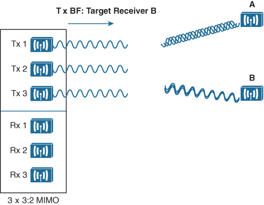
Figure 17-30 Using Transmit Beamforming to Target a Specific Receiving Device
The location and RF conditions can be unique for each receiver in an area. Therefore, transmit beamforming can use explicit feedback from the device at the far end, enabling the transmitter to make the appropriate adjustments to the transmitted signal phase. As T×BF information is collected about each far end device, a transmitter can keep a table of the devices and phase adjustments so that it can send focused transmissions to each one dynamically.
Maximal-Ratio Combining
When an RF signal is received on a device, it may look very little like the original transmitted signal. The signal may be degraded or distorted due to a variety of conditions. If that same signal can be transmitted over multiple antennas, as in the case of a MIMO device, then the receiving device can attempt to restore it to its original state.
The receiving device can use multiple antennas and radio chains to receive the multiple transmitted copies of the signal. One copy might be better than the others, or one copy might be better for a time, and then become worse than the others. In any event, maximal-ratio combining (MRC) can combine the copies to produce one signal that represents the best version at any given time. The end result is a reconstructed signal with an improved SNR and receiver sensitivity.
Maximizing the AP–Client Throughput
To pass data over an RF signal successfully, both a transmitter and receiver have to use the same modulation method. In addition, the pair should use the best data rate possible, given their current environment. If they are located in a noisy environment, where a low SNR or a low RSSI might result, a lower data rate might be preferable. If not, a higher data rate is better.
When wireless standards like 802.11n, 802.11ac, and 802.11ax offer many possible modulation methods and a vast number of different data rates, how do the transmitter and receiver select a common method to use? To complicate things, the transmitter, the receiver, or both might be mobile. As they move around, the SNR and RSSI conditions will likely change from one moment to the next. The most effective approach is to have the transmitter and receiver negotiate a modulation method (and the resulting data rate) dynamically, based on current RF conditions.
One simple solution to overcome free space path loss is to increase the transmitter’s output power. Increasing the antenna gain can also boost the EIRP. Having a greater signal strength before the free space path loss occurs translates to a greater RSSI value at a distant receiver after the loss. This approach might work fine for an isolated transmitter, but can cause interference problems when several transmitters are located in an area.
A more robust solution is to just cope with the effects of free space path loss and other detrimental conditions. Wireless devices are usually mobile and can move closer to or farther away from a transmitter at will. As a receiver gets closer to a transmitter, the RSSI increases. This, in turn, translates to an increased SNR. Remember that more complex modulation and coding schemes can be used to transport more data when the SNR is high. As a receiver gets farther away from a transmitter, the RSSI (and SNR) decreases. More basic modulation and coding schemes are needed there because of the increase in noise and the need to retransmit more data.
802.11 devices have a clever way to adjust their modulation and coding schemes based on the current RSSI and SNR conditions. If the conditions are favorable for good signal quality and higher data rates, a complex modulation and coding scheme (and a high data rate) is used. As the conditions deteriorate, less-complex schemes can be selected, resulting in a greater range but lower data rates. The scheme selection is commonly known as dynamic rate shifting (DRS). As its name implies, it can be performed dynamically with no manual intervention.
As a simple example, Figure 17-31 illustrates DRS operation on the 2.4 GHz band. Each concentric circle represents the range supported by a particular modulation and coding scheme. (You can ignore the cryptic names because they are beyond the scope of the ENCOR 350-401 exam.) The figure is somewhat simplistic because it assumes a consistent power level across all modulation types. Notice that the white circles denote OFDM modulation (802.11g), and the shaded circles contain DSSS modulation (802.11b). None of the 802.11n/ac/ax modulation types are shown, for simplicity. The data rates are arranged in order of increasing circle size or range from the transmitter.

Figure 17-31 Dynamic Rate Shifting as a Function of Range
Suppose that a mobile user starts out near the transmitter, within the innermost circle, where the received signal is strong and SNR is high. Most likely, wireless transmissions will use the OFDM 64-QAM 3/4 modulation and coding scheme to achieve a data rate of 54 Mbps. As the user walks away from the transmitter, the RSSI and SNR fall by some amount. The new RF conditions will likely trigger a shift to a different less complex modulation and coding scheme, resulting in a lower data rate.
In a nutshell, each move outward, into a larger concentric circle, causes a dynamic shift to a reduced data rate, in an effort to maintain the data integrity to the outer reaches of the transmitter’s range. As the mobile user moves back toward the AP again, the data rates will likely shift higher and higher again.
The same scenario in the 5 GHz band would look very similar, except that every circle would use an OFDM modulation scheme and data rate corresponding to 802.11a, 802.11n, 802.11ac, or 802.11ax.
Exam Preparation Tasks
As mentioned in the section “How to Use This Book” in the Introduction, you have a couple of choices for exam preparation: the exercises here, Chapter 30, “Final Preparation,” and the exam simulation questions in the Pearson Test Prep Software Online.
Review All Key Topics
Review the most important topics in this chapter, noted with the Key Topic icon in the outer margin of the page. Table 17-5 lists these key topics and the page number on which each is found.
Table 17-5 Key Topics for Chapter 17
Key Topic Element |
Description |
Page Number |
Paragraph |
dB definition |
492 |
List |
Important dB laws to remember |
492 |
Paragraph |
EIRP calculation |
496 |
List |
Free space path loss concepts |
498 |
Effective Range of 2.4 GHz and 5 GHz Transmitters |
499 |
|
Example of Receiver Sensitivity Level |
500 |
|
List |
Modulation scheme output |
502 |
A Summary of Common 802.11 Standard Amendments |
504 |
|
Dynamic Rate Shifting as a Function of Range |
509 |
Complete Tables and Lists from Memory
Print a copy of Appendix B, “Memory Tables” (found on the companion website), or at least the section for this chapter, and complete the tables and lists from memory. Appendix C, “Memory Tables Answer Key,” also on the companion website, includes completed tables and lists you can use to check your work.
Define Key Terms
Define the following key terms from this chapter and check your answers in the Glossary:
direct sequence spread spectrum (DSSS)
effective isotropic radiated power (EIRP)
Orthogonal Frequency Division Multiplexing (OFDM)
quadrature amplitude modulation (QAM)