Chapter 6
Integration by Parts
In This Chapter
![]() Making the connection between the Product Rule and integration by parts
Making the connection between the Product Rule and integration by parts
![]() Knowing how and when integration by parts works
Knowing how and when integration by parts works
![]() Integrating by parts by using the DI-agonal method
Integrating by parts by using the DI-agonal method
![]() Practicing the DI-agonal method on the four most common products of functions
Practicing the DI-agonal method on the four most common products of functions
In Calculus I, you find that the Product Rule allows you to find the derivative of any two functions that are multiplied together. (I review this in Chapter 2, in case you need a refresher.) But integrating the product of two functions isn’t quite as simple. Unfortunately, no formula allows you to integrate the product of any two functions. As a result, a variety of techniques have been developed to handle products of functions on a case-by-case basis.
In this chapter, I show you the most widely applicable technique for integrating products, called integration by parts. First, I demonstrate how the formula for integration by parts follows the Product Rule. Then I show you how the formula works in practice. After that, I give you a list of the products of functions that are likely to yield to this method.
After you understand the principle behind integration by parts, I give you a method — called the DI-agonal method — for performing this calculation efficiently and without errors. Then I show you examples of how to use this method to integrate the four most common products of functions.
Introducing Integration by Parts
Integration by parts is a happy consequence of the Product Rule (discussed in Chapter 2). In this section, I show you how to tweak the Product Rule to derive the formula for integration by parts. I show you two versions of this formula — a complicated version and a simpler one — and then recommend that you memorize the second. I show you how to use this formula, and then I give you a heads up as to when integration by parts is likely to work best.
Reversing the Product Rule
The Product Rule (see Chapter 2) enables you to differentiate the product of two functions:
![]()
Through a series of mathematical somersaults, you can turn this equation into a formula that’s useful for integrating. This derivation doesn’t have any truly difficult steps, but the notation along the way is mind-deadening, so don’t worry if you have trouble following it. Knowing how to derive the formula for integration by parts is less important than knowing when and how to use it, which I focus on in the rest of this chapter.
The first step is simple: Just rearrange the two products on the right side of the equation:
![]()
Next, rearrange the terms of the equation:
![]()
Now integrate both sides of this equation:
![]()
Use the Sum Rule to split the integral on the right in two:
![]()
The first of the two integrals on the right undoes the derivative:
![]()
This is the formula for integration by parts. But because it’s so hairy looking, the following substitution is used to simplify it:
Let u = f(x) Let v = g(x)
du = f'(x) dx dv = g'(x) dx
 Here’s the friendlier version of the same formula, which you should memorize:
![]()
Knowing how to integrate by parts
The formula for integration by parts gives you the option to break the product of two functions down to its factors and integrate it in an altered form.
To integrate by parts:
1. Decompose the entire integral (including dx) into two factors.
2. Let the factor without dx equal u and the factor with dx equal dv.
3. Differentiate u to find du, and integrate dv to find v.
4. Use the formula ![]() .
.
5. Evaluate the right side of this equation to solve the integral.
For example, suppose that you want to evaluate this integral:
![]()
In its current form, you can’t perform this computation, so integrate by parts:
1. Decompose the integral into ln x and x dx.
2. Let u = ln x and dv = x dx.
3. Differentiate ln x to find du and integrate x dx to find v:
Let u = ln x Let dv = x dx
![]()
![]()
![]()
![]()
4. Using these values for u, du, v, and dv, you can use the formula for integration by parts to rewrite the integral as follows:
![]()
At this point, algebra is useful to simplify the right side of the equation:
![]()
5. Evaluate the integral on the right:
![]()
You can simplify this answer just a bit:
![]()
To check this answer, differentiate it by using the Product Rule:
![]()
![]()
![]()
Now simplify this result to show that it’s equivalent to the function you started with:
![]()
Knowing when to integrate by parts
After you know the basic mechanics of integrating by parts, as I show you in the previous section, it’s important to recognize when integrating by parts is useful.
To start off, here are two important cases when integration by parts is definitely the way to go:
![]() The logarithmic function ln x
The logarithmic function ln x
![]() The first four inverse trig functions (arcsin x, arccos x, arctan x, and arccot x)
The first four inverse trig functions (arcsin x, arccos x, arctan x, and arccot x)
Beyond these cases, integration by parts is useful for integrating the product of more than one function. For example:
![]() x ln x
x ln x
![]() x arcsec x
x arcsec x
![]() x2 sin x
x2 sin x
![]() ex cos x
ex cos x
Notice that in each case, you can recognize the product of functions because the variable x appears more than once in the function.
 Whenever you’re faced with integrating the product of functions, consider variable substitution (which I discuss in Chapter 5) before you think about integration by parts. For example, x cos (x2) is a job for variable substitution, not integration by parts. (To see why, flip to Chapter 5.)
When you decide to use integration by parts, your next question is how to split up the function and assign the variables u and dv. Fortunately, a helpful mnemonic exists to make this decision: Lovely Integrals Are Terrific, which stands for Logarithmic, Inverse trig, Algebraic, Trig. (If you prefer, you can also use the mnemonic Lousy Integrals Are Terrible.) Always choose the first function in this list as the factor to set equal to u, and then set the rest of the product (including dx) equal to dv.
You can use integration by parts to integrate any of the functions listed in Table 6-1.

When you’re integrating by parts, here’s the most basic rule when deciding which term to integrate and which to differentiate: If you only know how to integrate one of the two, that’s the one you integrate!
Integrating by Parts with the DI-agonal Method
The DI-agonal method is basically integration by parts with a chart that helps you organize information. This method is especially useful when you need to integrate by parts more than once to solve a problem. In this section, I show you how to use the DI-agonal method to evaluate a variety of integrals.
Looking at the DI-agonal chart
The DI-agonal method avoids using u and dv, which are easily confused (especially if you write the letters u and v as sloppily as I do!). Instead, a column for differentiation is used in place of u, and a column for integration replaces dv.
Use the following chart for the DI-agonal method:

As you can see, the chart contains two columns: the D column for differentiation, which has a plus sign and a minus sign, and the I column for integration. You may also notice that the D and the I are placed diagonally in the chart — yes, the name DI-agonal method works on two levels (so to speak).
Using the DI-agonal method
Earlier in this chapter, I provide a list of functions that you can integrate by parts. The DI-agonal method works for all these functions. I also give you the mnemonic Lovely Integrals Are Terrific (which stands for Logarithmic, Inverse trig, Algebraic, Trig) to help you remember how to assign values of u and dv — that is, what to differentiate and what to integrate.
To use the DI-agonal method:
1. Write the value to differentiate in the box below the D and the value to integrate (omitting the dx) in the box below the I.
2. Differentiate down the D column and integrate down the I column.
3. Add the products of all full rows as terms.
I explain this step in further detail in the examples that follow.
4. Add the integral of the product of the two lowest diagonally adjacent boxes.
I also explain this step in greater detail in the examples.
Don’t spend too much time trying to figure this process out. The upcoming examples show you how it’s done and give you plenty of practice. I show you how to use the DI-agonal method to integrate products that include logarithmic, inverse trig, algebraic, and trig functions.
L is for logarithm
You can use the DI-agonal method to evaluate the product of a log function and an algebraic function. For example, suppose that you want to evaluate the following integral:
![]()
Whenever you integrate a product that includes a log function, the log function always goes in the D column.
1. Write the log function in the box below the D and the rest of the function value (omitting the dx) in the box below the I.
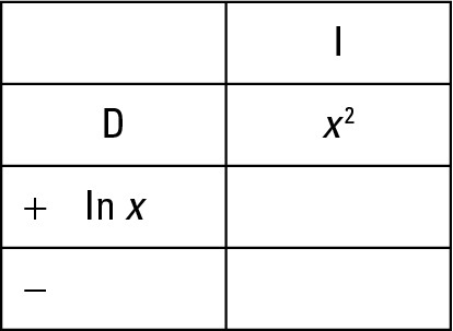
2. Differentiate ln x and place the answer in the D column.
Notice that in this step, the minus sign already in the box attaches to ![]() .
.

3. Integrate x2 and place the answer in the I column.

4. Add the product of the full row that’s circled.

Here’s what you write:
![]()
5. Add the integral of the two lowest diagonally adjacent boxes that are circled.

Here’s what you write:
![]()
At this point, you can simplify the first term and integrate the second term:
![]()
![]()
![]()
You can verify this answer by differentiating with the Product Rule:
![]()
![]()
![]()
![]()
Therefore, this is the correct answer:
![]()
I is for inverse trig
You can integrate four of the six inverse trig functions (arcsin x, arccos x, arctan x, and arccot x) using the DI-agonal method. By the way, if you haven’t memorized the derivatives of the six inverse trig functions (which I give you in Chapter 2), this would be a great time to do so.
Whenever you integrate a product that includes an inverse trig function, this function always goes in the D column.
For example, suppose that you want to integrate the following:
![]()
1. Write the inverse trig function in the box below the D and the rest of the function value (omitting the dx) in the box below the I.

Note that a 1 goes into the I column.
2. Differentiate arccos x and place the answer in the D column, and then integrate 1 and place the answer in the I column.

3. Add the product of the full row that’s circled.

Here’s what you write:
(+arccos x)(x)
4. Add the integral of the lowest diagonal that’s circled.

Here’s what you write:

Simplify and integrate:
Let u = 1 – x2
du = –2x dx
![]()
 This variable substitution introduces a new variable u. Don’t confuse this u with the u used for integration by parts.
![]()
![]()
![]()
Substituting 1 – x2 for u and simplifying gives you this answer:
![]()
Therefore, ![]() .
.
A is for algebraic
If you’re a bit skeptical that the DI-agonal method is really worth the trouble, I guarantee you that you’ll find it useful when handling algebraic factors.
For example, suppose that you want to integrate the following:
![]()
This example is a product of functions, so integration by parts is an option. Going down the LIAT checklist, you notice that the product doesn’t contain a log factor or an inverse trig factor. But it does include the algebraic factor x3, so place this factor in the D column and the rest in the I column. By now, you’re probably getting good at using the chart, so I fill it in for you here:

Your next step is normally to write the following:
![]()
But here comes trouble: The only way to calculate the new integral is by doing another integration by parts. And, peeking ahead a bit, here’s what you have to look forward to:
![]()
![]()
At last, after integrating by parts three times, you finally have an integral that you can solve directly. If evaluating this expression looks like fun (and if you think you can do it quickly on an exam without dropping a minus sign along the way!), by all means go for it. If not, I show you a better way. Read on.
To integrate an algebraic function multiplied by a sine, a cosine, or an exponential function, place the algebraic factor in the D column and the other factor in the I column. Differentiate the algebraic factor down to zero, and then integrate the other factor the same number of times. You can then copy the answer directly from the chart.
Simply extend the DI chart as I show you here:

Notice that you just continue the patterns in both columns. In the D column, continue alternating plus and minus signs and differentiate until you reach 0. And in the I column, continue integrating.
The very pleasant surprise is that you can now copy the answer from the chart. This answer contains four terms (+ C, of course), which I copy directly from the four circled rows in the chart:
x3 (–cos x) – 3x2 (–sin x) + 6x (cos x) – 6 (sin x) + C
But wait! Didn’t I forget the final integral on the diagonal? Actually, no — but this integral is ![]() , which explains where that final C comes from.
, which explains where that final C comes from.
Here’s another example, just to show you again how easy the DI-agonal method is for products with algebraic factors:
![]()
Without the DI chart, this problem is one gigantic miscalculation waiting to happen. But the chart keeps track of everything. Check it out:

Now just copy from the chart, add C, and simplify:
![]()
![]()
![]()
This answer is perfectly acceptable, but if you want to get fancy, factor out ![]() and leave a reduced polynomial:
and leave a reduced polynomial:
![]()
T is for trig
You can use the DI-agonal method to integrate the product of either a sine or a cosine and an exponential. For example, suppose that you want to evaluate the following integral:
![]()
When integrating either a sine or cosine function multiplied by an exponential function, make your DI-agonal chart with five rows rather than four. Then place the trig function in the D column and the exponential in the I column.

This time, you have two rows to add as well as the integral of the product of the lowest diagonal:
![]()
This may seem like a dead end because the resulting integral looks so similar to the one that you’re trying to evaluate. Oddly enough, however, this similarity makes solving the integral possible. In fact, the next step is to make the integral that results look exactly like the one you’re trying to solve:
![]()
Next, substitute the variable I for the integral that you’re trying to solve. This action isn’t strictly necessary, but it makes the course of action a little clearer.
![]()
Now solve for I using a little basic algebra:
![]()

Finally, substitute the original integral back into the equation, and add C:

Optionally, you can clean up this answer a bit by factoring:
![]()
If you’re skeptical that this method really gives you the right answer, check it by differentiating with the Product Rule:
![]()

At this point, algebra shows that this expression is equivalent to the original function:

![]()
![]()
![]()