
In the Parallelizing processing with pmap recipe we found that while using pmap is easy enough, knowing when to use it is more complicated. Processing each task in the collection has to take enough time to make the costs of threading, coordinating processing, and communicating the data worth it. Otherwise, the program will spend more time with how the parallelization is done and not enough time with what the task is.
A way to get around this is to make sure that pmap has enough to do at each step it parallelizes. The easiest way to do this is to partition the input collection into chunks and run pmap on groups of the input.
For this recipe, we'll use Monte Carlo methods to approximate pi. We'll compare a serial version against a naïve parallel version as well as a version that uses parallelization and partitions.
Monte Carlo methods work by attacking a deterministic problem, such as computing pi, nondeterministically. That is, we'll take a nonrandom problem and throw random data at it in order to compute the results. We'll see how this works and go into more detail on what this means toward the end of this recipe.
We'll use Criterium (https://github.com/hugoduncan/criterium) to handle benchmarking, so we'll need to include it as a dependency in our Leiningen project.clj file:
(defproject parallel-data "0.1.0"
  :dependencies [[org.clojure/clojure "1.6.0"]
                 [criterium "0.4.3"]])
We'll also use Criterium and the java.lang.Math class in our script or REPL:
(use 'criterium.core)
(import [java.lang Math])
To implement this, we'll define some core functions and then implement a Monte Carlo method that uses pmap to estimate pi.
- We need to define the functions that are necessary for the simulation. We'll have one function that generates a random two-dimensional point, which will fall somewhere in the unit square:
(defn rand-point [] [(rand) (rand)])
- Now, we need a function to return a point's distance from the origin:
(defn center-dist [[x y]]
  (Math/sqrt (+ (* x x) (* y y))))
- Next, we'll define a function that takes a number of points to process and creates that many random points. It will return the number of points that fall inside a circle:
(defn count-in-circle [n] (->> (repeatedly n rand-point) (map center-dist) (filter #(<= % 1.0)) count)) - This simplifies our definition of the base (serial) version. This calls
count-in-circleto get the proportion of random points in a unit square that fall inside a circle. It multiplies this by4, which should approximate pi:(defn mc-pi [n] (* 4.0 (/ (count-in-circle n) n)))
- We'll use a different approach for the simple
pmapversion. The function that we'll parallelize will take a point and either return1if it's in the circle, or it will return0if it is not. Then, we can add these up to find the number in the circle:(defn in-circle-flag [p] (if (<= (center-dist p) 1.0) 1 0)) (defn mc-pi-pmap [n] (let [in-circle (->> (repeatedly n rand-point) (pmap in-circle-flag) (reduce + 0))] (* 4.0 (/ in-circle n)))) - Moreover, for the version that chunks the input, we'll do something different again. Instead of creating a sequence of random points and partitioning it, we'll have a sequence that tells us how large each partition should be and have
pmapwalk across it, callingcount-in-circle. This means that the creation of larger sequences is also parallelized:(defn mc-pi-part ([n] (mc-pi-part 512 n)) ([chunk-size n] (let [step (int (Math/floor (float (/ n chunk-size)))) remainder (mod n chunk-size) parts (lazy-seq (cons remainder (repeat step chunk-size))) in-circle (reduce + 0 (pmap count-in-circle parts))] (* 4.0 (/ in-circle n)))))
Now, how well do these work? We'll bind our parameters to names, and then we'll run one set of benchmarks before we take a look at a table of all of them. We'll discuss the results in the next section.
user=> (def chunk-size 4096)
#'user/chunk-size
user=> (def input-size 1000000)
#'user/input-size
user=> (quick-bench (mc-pi input-size))
WARNING: Final GC required 3.825293394551939 % of runtime
Evaluation count : 6 in 6 samples of 1 calls.
Execution time mean : 354.953166 ms
Execution time std-deviation : 13.118006 ms
Execution time lower quantile : 345.135999 ms ( 2.5%)
Execution time upper quantile : 375.628874 ms (97.5%)
Overhead used : 1.871847 ns
Found 1 outliers in 6 samples (16.6667 %)
low-severe 1 (16.6667 %)
Variance from outliers : 13.8889 % Variance is moderately inflated by outliers
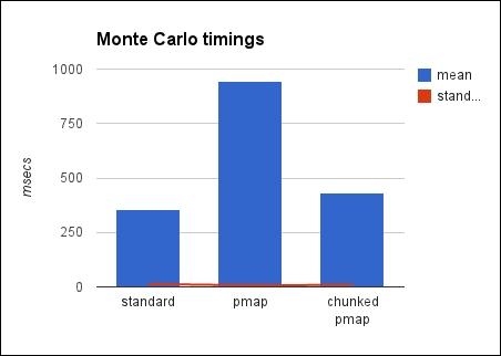
nilThe following table shows the timings of each way of running the program, along with the parameters given, if applicable:
|
Function |
Input size |
Chunk size |
Mean |
Std deviation |
GC time |
|---|---|---|---|---|---|
|
|
1,000,000 |
NA |
354.953ms |
13.118ms |
3.825% |
|
|
1,000,000 |
NA |
944.230ms |
7.363ms |
1.588% |
|
|
1,000,000 |
4,096 |
430.404ms |
8.952ms |
3.303% |
Here's a chart with the same information:
There are a couple of things we should talk about here. Primarily, we need to look at chunking the inputs for pmap, but we should also discuss Monte Carlo methods.
Monte Carlo simulations work by throwing random data at a problem that is fundamentally deterministic and when it's practically infeasible to attempt a more straightforward solution. Calculating pi is one example of this. By randomly filling in points in a unit square, π/4 will be approximately the ratio of the points that fall within a circle centered at 0, 0. The more random points we use, the better the approximation is.
Note that this is a good demonstration of Monte Carlo methods, but it's a terrible way to calculate pi. It tends to be both slower and less accurate than other methods.
Although not good for this task, Monte Carlo methods are used for designing heat shields, simulating pollution, ray tracing, financial option pricing, evaluating business or financial products, and many other things.
Note
For a more in-depth discussion, you can refer to Wikipedia, which has a good introduction to Monte Carlo methods, at http://en.wikipedia.org/wiki/Monte_Carlo_method.
The table present in this section makes it clear that partitioning helps. The partitioned version took roughly the same amount of time as the serial version, while the naïve parallel version took almost three times longer.
The speedup between the naïve and chunked parallel versions is because each thread is able to spend longer on each task. There is a performance penalty on spreading the work over multiple threads. Context switching (that is, switching between threads) costs time as does coordinating between threads. However, we expect to be able to make that time (and more) by doing more things at once.
However, if each task itself doesn't take long enough, then the benefit won't outweigh the costs. Chunking the input, and effectively creating larger individual tasks for each thread, gets around this by giving each thread more to do, thereby spending less time in context switching and coordinating, relative to the overall time spent in running.