
Chapter 5
Simple Transport Protocol
5.1. Introduction
Transport protocols hide all the possible problems inherent to the physical and network layers, such as disorder, losses, delay and corruption. These protocols provide a reliable and ordered communication between a sender and a receiver, the usual strategy being to retransmit a lost or corrupted packet. At the same time, the most sophisticated of these protocols implement different mechanisms in order to avoid duplication and ensure correct delivery order, and to optimize the performance of data delivery versus the underlying real or virtual network.
In this section, we will create our own, simple transport protocol to provide a correct order and reliability to the user layers when transmitting a set of messages over a Non-Reliable Medium. To do this, we will use the well-known basic algorithm called the Alternating Bit Protocol.
To reach this goal, this chapter builds a system architecture by linking the Simple Chat Application modeled in Chapter 3 to the Non-Reliable Medium modeled in Chapter 4, through a Simple Transport Protocol.
Of course, to do so, it will be necessary to slightly adapt and modify the precedent models, and to extend the characteristics of the transmitted data type.
5.2. Requirements
Two remote chat applications need to communicate through a Non-Reliable Medium, and we therefore propose a transport protocol with the following characteristics:
– the protocol will offer a reliable and ordered communication service to its application;
– the protocol will support a full duplex (bidirectional) communication;
– the protocol will ensure the correct delivery of a data packet before accepting a new data packet to transmit, i.e. it accepts and transmits one single packet at a time from the application;
– the protocol instances communicate through a Non-Reliable Medium;
– the protocol will implement the Alternating Bit mechanism in order to solve packets losses and delays;
– the communication interfaces of the application and the medium are already defined because the modules already exist, and the transport protocol will use the interfaces defined in those modules.
5.3. The Alternating Bit Protocol
The Alternating Bit Protocol (ABP) is a reliable transport protocol solving the problem of transferring data from a sender A to a receiver B through a Non-Reliable Medium. As it is simple and very illustrative (although not efficient), we will use it in order to show how to design such a transport protocol and how to link it to its adjacent layers.
First we will describe the Alternating Bit Protocol by using the Petri Nets formalism, since this is one of the traditional representations of this algorithm in the network context. After that, we will explain how to model this algorithm in UML.
But before presenting the algorithm, let us recall some of the Petri Net notions needed for correct understanding of the ABP’s behavior and of the Petri Net model deduced.
5.3.1. Basic communication features with Petri Nets
We can represent the sending and receiving process actions by using Petri Nets, as shown in Figure 5.1.
In this figure, the transition labeled !E represents the execution of the sending process of data E, while the transition labeled ?E represents the execution of the receiving process of data E. As you can see, in this model, there is no explicit link between the sender and the receiver, i.e. the underlying sending-receiving interaction is not represented.
Figure 5.1. Simple transport protocol. Alternating bit protocol, representing data sent and received in Petri Nets
We can also represent the same behavior with an explicit representation of the sending-receiving interaction by adding a place E between the sender and the receiver, as shown in Figure 5.2. A mark or a “token”, as explained in section 1.1.2.2.2, in this new place represents that the data was sent by the sender, and that it has not yet been received; in other words, it represents the fact that the message is in transit in the communication medium (or the network).
Figure 5.2. Simple transport protocol. Alternating bit protocol: sending and receiving with a shared place
Figure 5.2 represents a shared-place communication. Indeed, a token in this place allows the firing of transition ?E. When !E is fired, the token is removed from place Sender, and one token is added to each of the two places that are the outputs of the transition !E, including place E. A token in place E means that the message is in transit in the medium. Transition ?E can now be fired since there is a token on each input place in this transition. Firing this transition means that the message is being received. After firing ?E, the two tokens are removed from the places Receiver and E, and one token is added in the output place of transition ?E. This means that the receiver has received the message and that is going to process it.
By using the same mechanism, we can represent a very simple protocol defining an entity sending a data packet and waiting for an acknowledgement answer, as shown in Figure 5.3.
Observe that, on the right side, the Receiver sends an acknowledgement ackE message. This action is represented by the transition labeled !ackE. On the left, the reception of the ackE message is represented by the transition labeled ?ackE. In the middle, a token in the place labeled ackE represents that the acknowledgement message was sent but is still not received; in other words, it is in transit through the communication medium.
Figure 5.3. Simple transport protocol. Alternating bit protocol: sending data and waiting for acknowledgement
In a real communication network, the data packets may be lost.
Figure 5.4 shows the Petri Net of Figure 5.2, extended to describe the data losses.
Let us observe the new transition, labeled “Loss”. The firing of this transition, which is possible when there is a token in place E (i.e. a message in transit), represents the medium losing the data stored in place E, as the token is removed from place E and will disappear.
Note that there are two possible behaviors when place E is marked: either transition “Loss” is fired and the message is lost, or transition ?E is fired, and the message is received. These are the two possible behaviors that our simple protocol has to handle when messages can be lost.
Figure 5.4. Simple transport protocol. Alternating bit protocol: representing a loss

In this model, if the data packet E is lost, then the ?E transition cannot be fired by the receiver and the system is blocked. Under these circumstances, the sender needs to resend the data packet. Figure 5.5 shows a new model where the firing of the “Loss” transition brings a mark back to the initial place on the sender’s side. This mark allows the sender to send a data packet again. Note that this process is repeated as long as the data packet is lost.
Note that the acknowledge packet might be lost by the medium in the same manner as the data packet. On the sender side, the only observable event is a missing acknowledgement packet. The problem here is that the sender cannot know if the lost message was the E data packet or the acknowledgement. However, in both circumstances, the sender needs to resend the data packet.
Figure 5.5. Simple transport protocol. Alternating bit protocol: resending data after a loss
Figure 5.6. Simple transport protocol. Alternating bit protocol: recovering from a loss
Figure 5.6 represents the loss of the acknowledgement as a new transition labeled “Lose-ack”. At the same time, we have renamed the transition representing the loss of the E data packet as “Lose-E”. Finally, we have represented the loss of either of these two messages as a new place, labeled “loss”. Note that this new place can receive a token from either Lose-E or Lose-ack transitions. A token in this loss place, while the sender is in the middle left state (message sent but not yet acknowledged), allows the firing of the transition Rs-E, and this transition leads to the sender place and to the retransmission of the data packet.
This model seems to work correctly. However, it presents a problem when the ackE packet is lost. Consider the following scenario:
– the sender sends a data packet (transition !E is fired);
– the data is received on the receiver side (transition ?E is fired);
– the receiver sends an ackE packet (transition !ackE is fired);
– the acknowledgement packet is lost (transition Lose-ack is fired);
– the sender is allowed to resend data (transition Rs-E is fired);
– the sender sends a data packet (transition !E is fired);
– the data is received on the receiver side (transition ?E is fired);
– the receiver sends an ackE packet (transition !ackE is fired).
Figure 5.7. Simple transport protocol. Alternating bit protocol: avoiding duplicated data
At this point, the data packet E is received twice by the receiver. We need a mechanism to detect that the data packet was already received by the receiver.
Figure 5.7 shows a new model with a solution to the previous problem. Observe that there is a new transition labeled “Rs-ack”. Note that this transition is enabled only when a data packet is in transit through the network and an acknowledgement packet was already sent by the receiver.
Observe that the firing of this transition has to be defined in such a way that the receiver must ignore the duplicated packet and retransmit the acknowledgement packet by firing the transition !ackE again.
5.3.2. The algorithm
The algorithm of the Alternating Bit Protocol (ABP) has to provide a reliable transport protocol solving the problem of transferring data in a unidirectional mode from a sender A to a receiver B through a Non-Reliable Medium. Note that it is a simplified form of the well-known Sliding Window mechanism with a window size of 1.
The ABP algorithm creates data packets containing the payload to be transferred. It then associates a control bit with each data packet, and the control bit is used to ensure a correct delivery order simply alternates between 0 and 1.
It also uses positive acknowledgements (ACK) in order to confirm the reception of data. Indeed, only one bit is needed since no new data is sent before acknowledgement of the previous data packet is received by the sender (stop-and-wait).
To begin, sender A sends a data packet (payload + control bit) and continues sending the same data at a regular frequency. Sender A stops sending the data packet when it receives an acknowledgement containing the same control bit from receiver B. After that, sender A complements (flips) the control bit and starts sending the next data packet containing the new control bit.
On the receiver side, on receipt of a data packet from sender A, receiver B sends back an acknowledgement packet containing the control bit that is included in the received message.
The first time B receives a message with a given control bit, it sends the payload to its receiver client for processing. If subsequent data packets containing the same control bit are received, they are only acknowledged (without delivering the message to the client).
Figure 5.8 shows a representation of the ABP [DIA 09]. Note that this model is an extension of the one presented in Figure 5.7.
Figure 5.8. Simple transport protocol. Algorithm for the ABP
In this new model, we represent a data packet containing a payload and a control bit as two transitions labeled E0 (!E0 for sending and ?E0 for receiving) for the data packet containing the control bit 0, and E1 (!E1 for sending and ?E1 for receiving) for the data packet containing the control bit 1. Note that the transitions labeled ?E0 and ?E1 represent the receiver reading the payload from a data packet and sending it to its client for processing. Note also that the sender does not send any further message before receipt of an acknowledgement for the currently sent data packet. Finally, observe that the sender and the receiver come back to their initial state after receipt of ackE1.
We can represent the same algorithm by using two separate state machines, one for the sender and one for the receiver. For simplicity’s sake, we will represent the exchanged information as only E(ControlBit) and Ack(ControlBit). We will add the details concerning the payload in a later section when defining the protocol behavior.
Figure 5.9 shows a simple state machine representing the sender. Note here that the sender resends the data only when its internal timer is over or when it receives an unexpected message from the receiver (states St_WaitingAck_0 and St_WaitingAck_1). After receiving the expected Ack message, the sender waits for a new data packet from its sender application (states St_WaitingData-0 and St_WaitingData-1). Any Ack is ignored while waiting for a new data.
Figure 5.9. Simple transport protocol. Sender’s behavior for the ABP
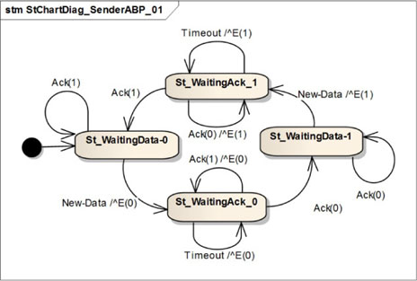
Figure 5.10 shows a simple state machine representing the receiver behavior. Observe that the receiver only processes the received data the first time; after that, it acknowledges the data packet but does not process it.
Figure 5.10. Simple transport protocol. Receiver’s behavior for ABP

5.4. Analysis
We will follow an iterative and incremental approach in order to analyze our system. This strategy will allow us to find the expected interfaces, their messages and some accessory classes.
5.4.1. First step: The Alternating Bit Protocol
We will now analyze the messages sent and received by the ABP without taking into account the application and the Non-Reliable Medium. The simplest way to do this is to consider the Alternating Bit Protocol Sender (ABPS) and the Alternating Bit Protocol Receiver (ABPR) as two separate systems. By doing so, we obtain two sets of messages.
Figure 5.11 shows the messages sent and received by the ABPS. Note that this diagram represents the sending process of a single data packet and does not take into account the change of the Control Bit (CB). Observe that this diagram corresponds to the Petri Nets model described in section 5.3.2.
User_A sends a data packet to the ABPS. Then, the ABPS sets its internal timer (message 2) and sends an E message containing a control bit and the received data to the ABPR (message 3). While no correct acknowledgement is received after a given time (timeout in message 4, and erroneous CB in message 6), the ABPS sends the E message again (messages 5 and 7). Finally, on the receipt of an acknowledgement message containing the expected CB (message 8), the ABPS resets its timer (message 9) and waits for a new data from the user.
Figure 5.11. Simple transport protocol. Sequence diagram for an Alternating Bit Protocol Sender (ABPS)
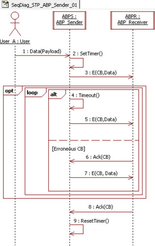
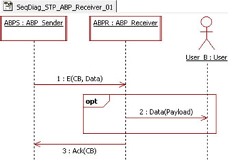
Figure 5.12 shows the messages sent and received by the ABPR. On receipt of an E packet, if the received data was not previously received, then the ABPR delivers the received data to its user; otherwise, the data is ignored. In any case, the received message is acknowledged with the received CB.
Figure 5.12. Simple transport protocol. Sequence diagram for an Alternating Bit Protocol Receiver (ABPR)
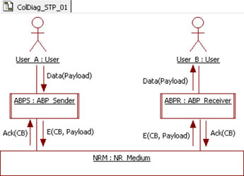
These sequence diagrams lead us to believe that the set of exchanged messages is as shown in Figure 5.13.
In this diagram we can see that the ABPS receives Data(Payload) from the user. It also sends E(CB, Payload) and receives Ack(CB) to/from the NRM.
The ABPR sends Data(Payload) to the user. It also sends Ack(CB) and receives E(CB, Payload) from the NRM.
Figure 5.13. Simple transport protocol. Messages exchanged between the ABP and its actors
However, it is not a (virtual) user who sends data to the protocol, but an already implemented application, here a chat application. This application has a well defined interface and our protocol must use it.
5.4.2. Second step: Linking the application
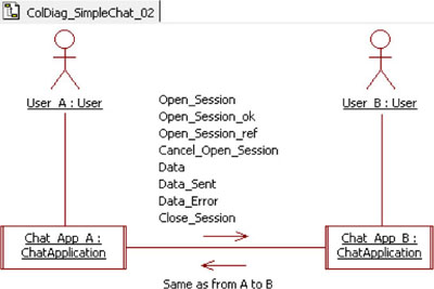
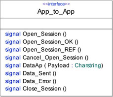
Figure 5.14 recalls the messages sent and read by the current chat application model (defined in section 3.3.3). Note that there are eight different messages exchanged between the two instances of the chat application.
Figure 5.14. Simple chat. List of messages between chat application instances
We can modify the data packet in order to add a payload. Let us say that the payload carried by this packet is a character string. By doing so, the new data packet will be defined as Data(Charstring: Payload). The rest of the messages will remain as they are.
Observe that the messages received by the ABPS and those sent by the ABPR are much more complex than simply Data(payload).
Currently, the ABPS only reads Data(payload) from the application and sends E(CB, Payload) to the ABPR. If we want the ABPS to read all the possible messages from the application, then we will need to create and manage many messages from ABPS to ABPR, i.e. E(CB, Open_Session), E(CB, Close_Session), E(CB, Data(Payload)), etc.
However, remember that our protocol must be indifferent to the transported data. In order to avoid a complicated algorithm, we need to define an encapsulating packet able to represent any of the application packets, in an homogeneous and general way.
To do so, we can create an Application Data Unit (ADU). An ADU contains a description of the represented message and of the payload carried. The structure of an ADU is as follows: ADU(Header, Payload). This way, a message Data(Payload) coming from the application corresponds to ADU(“Data”, Payload); the Open_Session message corresponds to an ADU(“Open_Session”, Empty_payload), etc.
We can also create a new module named ADU_Manager (ADUM), as we do not want to interrupt the ABPS and ABPR modules with more responsibilities and actions than necessary. The new specialized module which we create will translate the messages coming from the application into Application Data Units and vice versa.
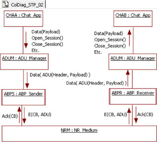
Figure 5.15 shows a new collaboration diagram depicting the messages exchanged between the ABP modules and the new ADUM. Note that the ABPS now receives a Data(ADU) message from the ADUM while the ABPR sends the same message to the ADUM. We should also note here that the old E(CB, Payload) message becomes E(CB, ADU). Thus, the behavior of the ABP modules remain unchanged.
Figure 5.15. Simple transport protocol. Messages exchanged between ABP and ADUM
5.4.3. Third step: Linking the medium
Now, we can link the protocol model to the Non-Reliable Medium (NRM). The NRM has a well defined interface, described in section 4.3.3. Figure 5.16 recalls the messages sent and received by the NRM.
Figure 5.16. Non-reliable medium. Messages exchanged between the medium and its actors
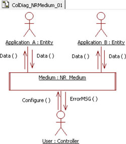
Observe that the current NRM model receives and sends a unique message to the entities: the Data() packet. Moreover, remember that the NRM does not read or process the received data, as it only transfers (or not) the received information from one port to another.
Conversely, the ABP modules send two kinds of messages to the medium, E(CB, ADU) and Ack(CB).
If we leave the ABPS and ABPR modules as they are now, then we will need to update the NRM model in order to add more information to the data packet. In addition, we will need to create a different data packet for every packet coming from the ABP modules.
We can simplify and homogenize the communication between the ABP modules and the medium by changing the current medium as little as possible.
First, we can modify the data packet in order to add a payload to it. After that, we can create a new data type called a Protocol Data Unit (PDU). A PDU encapsulates the packets sent and received by the medium. The structure of a PDU is defined as follows: PDU(Header, CB, ADU). In this way, the packet E(CB, ADU) corresponds to PDU(“E”, CB, ADU), while the Ack(CB) packet corresponds to PDU(“Ack”, CB, Empty_ADU). From this, the packets sent to the medium will be as simple as Data(PDU). In this way, with minimal modification, we can encapsulate all the information exchanged between the ABP modules.
We do not want to complicate the modules implementing the ABP algorithm by adding encapsulating behavior. Instead, we can create a new module named PDU_Manager (PDUM). This new module translates the messages exchanged between the ABPS and the ABPR into PDUs and sends them to the medium. In the reverse direction, the PDUM translates the PDU packets coming from the medium into E and Ack messages, and sends them to its corresponding algorithm module.
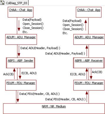
Figure 5.17 shows the new list of messages exchanged including the new PDUM module.
Figure 5.17. Simple transport protocol. Messages exchanged between PDUM and NRM
5.4.4. Concerned classes
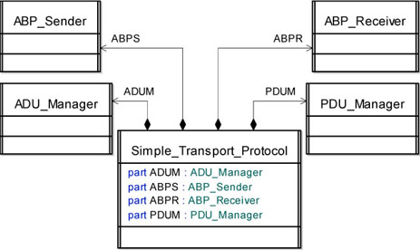
Our current model is composed of four different classes, ADU_Manager, PDU_Manager, ABP_Sender and ABP_Receiver.
We can add one more class and call it Simple_Transport_Protocol (STP). This new class is a container encapsulating all the transport protocol behavior and architecture.
The class diagram describing the relationship between these classes is shown in Figure 5.18. Note that all the classes are related to the container through a composition association.
Figure 5.18. Simple transport protocol. Class diagram representing the Simple Transport Protocol
We also need to define two data types representing the encapsulated data used in our model.
Figure 5.19 shows these two data types. Observe that PDU is related to ADU by a composition association.
Note that the payload in ADU and the header in both classes are defined as a character string. This is not the most efficient solution, but it will allow us to better read the simulation results.
Figure 5.19. Simple transport protocol. Encapsulated data used by the simple transport protocol

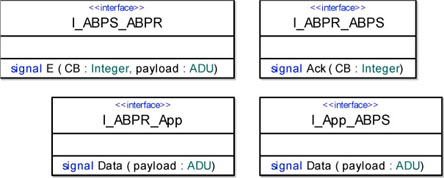
5.4.5. Signal list definition
The ABPS sends a packet E(CB, ADU) towards the ABPR. We can gather this packet into an interface called I_ABPS_ABPR. Figure 5.20 shows a detailed description of this interface. Remember that this message is translated into a PDU by the PDUM.
The ABPR sends a packet Ack(CB) towards the ABPS. We gather this packet into an interface called I_ABPR_ABPS. This message is translated into a PDU by the PDUM.
The ABPS receives a Data(ADU) packet from the application. Remember that the ADUM intercepts the messages coming from the application and translates them into ADUs. We can gather this packet into an interface called I_App_ABPS.
Finally, the ABPR sends a Data(ADU) packet towards the application. This packet is translated into application-styled packets by the ADUM. We will gather this packet into an interface called I_ABPR_App.
Figure 5.20. Simple transport protocol. Interfaces used by the simple transport protocol
We will use the interfaces defined previously in section 4.3.3 to communicate with the NRM. We can modify the Data packet in order to add a payload. The new interface list is shown in Figure 5.21.
Note that we changed the name of the data packet to Data_AtM and Data_MtA. This modification allows us to facilitate the reading of the simulation results by differentiating this packet from the other data packets.
Figure 5.21. Simple transport protocol. Modified interfaces for a non-reliable medium

Finally, we can use the interface defined in section 3.3.3 to communicate with the chat applications. We can modify the data packet in order to add a payload.
Note that, additionally, we have modified the name of the data packet to DataAp (Figure 5.22). This modification facilitates the reading of the resulting simulations by differentiating this data packet from those sent by other modules.
Figure 5.22. Simple transport protocol. Modified interface for the chat application
5.5. Architecture design
5.5.1. Simple transport protocol
We can now organize the classes composing the STP, starting with the ADUM.
In Figure 5.23 we can see that we added three ports to the ADUM module: P_ADUM_APP to communicate with the application, P_ADUM_ABPS to communicate with the Alternating Bit Protocol Sender, and P_ADUM_ABPR to communicate with the Alternating Bit Protocol Receiver.
Figure 5.23. Simple transport protocol. Ports and interfaces for the classes composing the simple transport protocol
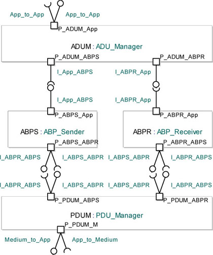
Observe the interfaces associated with each port. Note, for example, that the P_ADUM_ABPS port has no input interface since the ABPS is not supposed to send any information to the ADUM. Conversely, the P_ADUM_ABPR port has no output interface since it is not supposed to send any information through this port.
Now, let us take a look at the ABPS module. We added two ports to this class: P_ABPS_App to communicate with the ADUM module, and P_ABPS_ABPR in order to manage the communication with ABPR. Note that we will connect the P_ABPS_ABPR port to the PDUM module. Also note that this port sends E packets and receives Ack packets.
We can now analyze the ABPR module. We added two ports to this class: P_ABPR_App to send information to the ADUM module, and P_ABPR_ABPS to manage communication with the sender. Note that the P_ABPR_ABPS port receives E packets and sends Ack packets.
Finally, we can analyze the PDUM module. We added three ports to this class: P_PDUM_ABPS to communicate with the ABPS module, P_PDUM_ABPR to communicate with the receiver, and P_PDUM_M to communicate with the medium. Note that this class sends and receives PDUs to and from the medium.
Now, we can connect all the ports, between them and to the external world. Figure 5.24 shows how these classes are structured inside the Simple Transport Protocol module.
Figure 5.24. Simple transport protocol. Connecting the modules composing the simple transport protocol
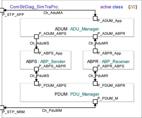
The external square represents the STP class borders. Note that we added two ports to the STP class: P_STP_APP to communicate with the application and P_STP_NRM to communicate with the Non-Reliable Medium.
Observe that the Ch_AduMS and Ch_AduMR channels are unidirectional and that they connect the ADUM module to ABPS and ABPR.
Finally, let us remark that the Ch_PduMM channel connects the PDUM module to the external world. This channel transports the packets going to and coming from the Non-Reliable Medium.
5.5.2. Simulation model
In order to build and simulate the resulting global model, we need to connect the STP module to the chat application and the Non-Reliable Medium.
Figure 5.25 shows the architecture that we will use for simulating and validating the Simple Transport Protocol.
Figure 5.25. Simple transport protocol. Ports and interfaces for simulating the STP
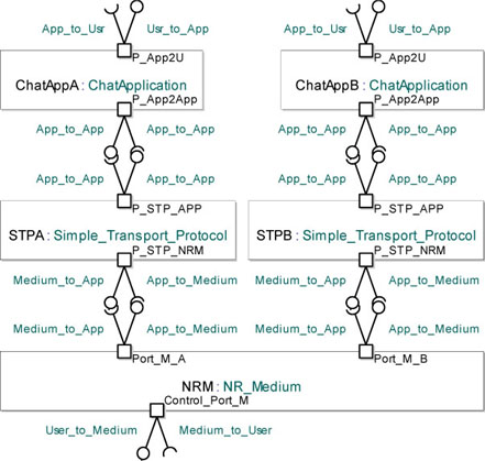
In particular, it describes the ports and the interfaces assigned to each class.
Observe that we created two instances of the ChatApplication class, ChatAppA and ChatAppB, and also note the coherence in the interfaces used to communicate with the STP instances.
We should note that we have also created two different instances of the Simple_Transport_Protocols class, STPA and STPB. Each instance is used by a different instance of the ChatApplication class.
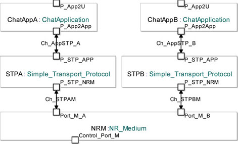
Figure 5.26 shows how the modules involved in the simulation are interconnected.
Figure 5.26. Simple transport protocol. Architecture used to simulate the STP
5.6. Detailed design
5.6.1. ADU data type
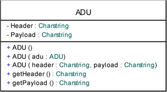
The ADU data type is composed of two char strings: the Header and the Payload. The Header contains the name of the message represented by the ADU. The Payload contains the payload carried by the data packet.
We now need to define a basic constructor1 creating an empty ADU, and also define an empty ADU as ADU(“”, “”).
We also need to define two more constructors: ADU(ADU) which will create a new ADU by copying the parameters of the ADU received; and ADU(header, payload) which will create a new ADU with the received parameters.
Finally, we must define two operations retrieving the internal attributes (commonly called getters): getHeader() and getPayload().
Figure 5.27 shows the detailed ADU class with its attributes and operations.
Figure 5.27. Simple transport protocol. Detailed ADU class with attributes and operations
5.6.2. PDU data type
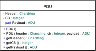
The PDU data type is composed of three attributes: Header, control bit (CB) and Payload. Remember that the payload in a PDU is of type ADU.
We must define three getters in order to retrieve the private attributes: getHeader(), getCB(), and getPayload().
We also need to define two creators: PDU(header, cb, payload) which will create a new PDU based on the received parameters; and PDU() will create an empty PDU. We can define an empty PDU as PDU(“”, 999, EMPTY_ADU).
Figure 5.28 shows the detailed PDU class with its attributes and operations.
Figure 5.28. Simple transport protocol. Detailed PDU class with attributes and operations
5.6.3. ADU_Manager
Most of the behavior of the ADU_Manager consists of translating every message received from the application into an ADU. The ADUM translates every message into a string of characters and assigns it to the header attribute in the ADU. Then, it assigns the payload (if any) to the Payload attribute.
The state machines for the ADU_Manager use three auxiliary variables: Payload, adu and header (see note (1) in Figure 5.29).
Figure 5.29. Simple transport protocol. ADUM: translating the Open_Session packet into an ADU
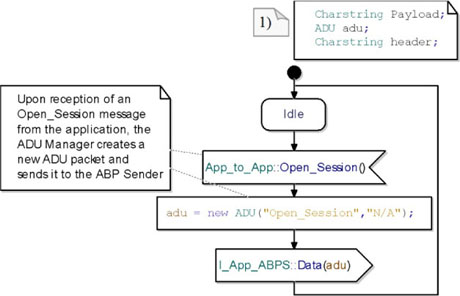
The ADU_Manager starts in an idle state. On receipt of an Open_Session message from the Chat_Application, it creates a new ADU with an empty payload (represented by the string “n/A”). Then, it sends a Data(ADU) packet to the Alternating Bit Protocol Sender.
Finally, it comes back to the idle state and waits for a new stimulus from either the chat application or the receiver.
Figure 5.30 shows the state machine translating the Data packet received from the Chat_Application. On receipt of this packet, it creates a new ADU with the received payload. Then, it sends the new ADU in a Data packet to the ABPS.
Finally, it comes back to the idle state and waits for a new packet to translate.
Figure 5.30. Simple transport protocol. ADUM: translating the Data packet into an ADU
The rest of the packets coming from the Chat_Application are translated using the same structure.
The state machines representing these translations are presented in section A.1 in the Appendix.
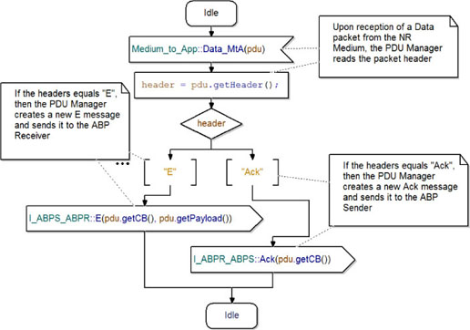
Figure 5.31 shows the state machine translating the packets coming from the Alternating Bit Protocol Receiver.
On receipt of a data packet, the system reads the header (see note (1)). After that, the ADUM translates the received header into the corresponding packet and sends it to the Chat_Application. Note that the ADUM additionally reads the payload (see note (2)) when the received header is Data.
Figure 5.31. Simple transport protocol. ADUM: translating ADU into original packets

5.6.4. PDU_Manager
The work of the PDU manager consists of translating all the messages coming from and going to the ABPS and ABPR into PDUs and vice versa. The PDUM translates every message into a string of characters and assigns it to the Header attribute in the PDU. After that, it adds the Control Bit (CB) and the payload and sends it to the medium.
In the opposite direction, the PDUM extracts all the fields from a PDU and creates simple messages; then, it sends the packet to either the ABPS or ABPR.
The state machines of the PDUM use four auxiliary variables: CB, pdu, header and adu (see note (1) in Figure 5.32).
Figure 5.32 shows the translation of an E packet into a PDU. On receipt of an E packet, the PDUM creates a PDU with the received values. After that, it sends the new PDU to the Non-Reliable Medium. Finally, it comes back to its idle state and waits for a new message to translate. Note that the PDUM does not analyze the received CB or ADU; instead, it only uses them to construct a new PDU.
Figure 5.32. Simple transport protocol. Translation of an E packet into a PDU
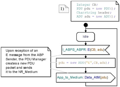
Figure 5.33 shows the translation of an Ack packet into a PDU. On receipt of an Ack packet, the PDUM creates a new PDU with en empty ADU as its payload. After that, it sends the new PDU to the Non-Reliable Medium.
Finally, it returns to its idle state and waits for a new message to translate.
Figure 5.33. Simple transport protocol. Translation of an Ack packet into a PDU
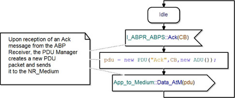
Figure 5.34 shows the state machine translating a PDU into an E or Ack packet. On receipt of a data packet from the medium, the PDUM reads the header. It then creates the correct packet and sends it to the ABPS or ABPR modules.
Finally, it goes back to the idle state and waits for another packet to translate.
Figure 5.34. Simple Transport Protocol. Translation of a PDU into an E or Ack packet
5.6.5. ABP_Sender
The ABP_Sender class uses an internal attribute to define the time it will wait until re-sending the E packet when no answer is received from the ABPR. We can call this attribute Maximum Round Trip Time (RTT).
The sender also needs a timer. We will call this timer timerABPS.
Figure 5.35 shows the detailed ABP_Sender class with attributes and operations.
Figure 5.35. Simple Transport Protocol. Detailed ABP_Sender class with attributes and operations
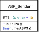
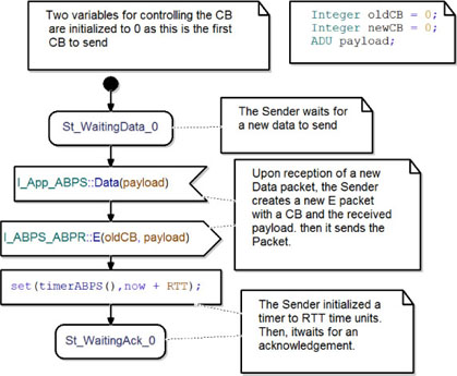
Figure 5.36 shows the behavior of the ABPS when it is waiting for a first data to send. The system starts in the St_WaitingData_0 state. On receipt of a data packet from the ADUM, it sends an E packet to the PDUM with CB equal to 0 and the received ADU (observe the initialization of the oldCB variable). After that, the ABPS sets its timer to now + RTT. Finally, it goes to the St_WaitingAck_0 state and waits for an acknowledgement from the Alternating Bit Protocol Receiver.
Figure 5.36. Simple transport protocol ABP_Sender class waiting for the first data to send
If the ABPS receives an unexpected acknowledgement while waiting for a new data, it simply ignores it. This behavior is represented in Figure 5.37.
Figure 5.37. Simple transport protocol. ABP_Sender class ignoring unexpected acknowledgements while waiting for new data
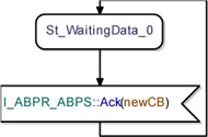
Figure 5.38 shows the behavior of the ABPS class when it is in the St_WaitingAck_0 state and receives an Ack packet from the ABPR.
Figure 5.38. Simple transport protocol. ABP_Sender class waiting for the Ack(0) from the ABPR
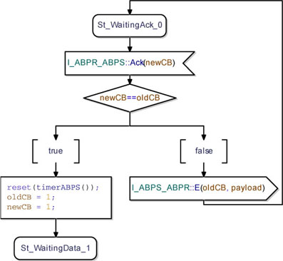
On receipt of an Ack packet, the ABPS reads the received CB. Then, it compares it with the last CB sent.
If the received CB is equal to the expected one, then the ABPS resets its timer. After that, it updates its internal CB variables and waits for a new data to send.
If the received CB is not equal to the expected one, then the ABPS re-sends the E packet to the PDUM and goes back to waiting for the expected acknowledgement.
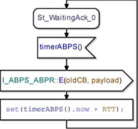
If the ABPS is waiting for an Ack(0) from the ABPR and the internal timeout signal is triggered, then the ABPS re-sends the E packet to the PDUM and sets its timer again. After that, it goes back to waiting for a correct answer from the ABPR. Figure 5.39 shows the state machine modeling this behavior.
Figure 5.39. Simple transport protocol. ABP_Sender class: timeout when waiting for Ack(0)
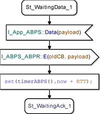
After reception of the acknowledgement of the E packet with CB 0, the ABPS waits for a new data to send. When it receives a new data packet from the ADUM, the ABPS sends an E packet to the PDUM with CB equal to 1 and the received payload. After that, it sets its timer to now + RTT. Finally, it waits for an acknowledgement from the ABPR. Figure 5.40 shows the state machine modeling this behavior.
Figure 5.40. Simple transport protocol. ABP_Sender class waiting for the second data to send
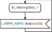
If the ABPS receives an unexpected acknowledgement while waiting for a new data, it simply ignores it. This behavior is represented in Figure 5.41.
Figure 5.41. Simple transport protocol. ABP_Sender class ignoring unexpected acknowledgements while waiting for new data
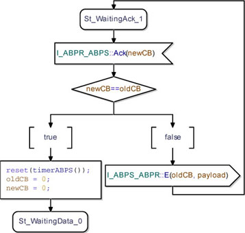
When the ABPS is in the St_WaitingAck_1 state and it receives an Ack packet, it reads the received CB and compares with the last CB sent. If this is equal to the one expected, it resets its timer and updates its internal variables. After that, it goes to the initial state. If the received CB is not equal to the expected one, then it re-sends the E packet to the PDUM and goes back to waiting for the correct acknowledge packet. Figure 5.42 shows the state machine implementing this behavior.
Figure 5.42. Simple transport protocol. ABP_Sender class waiting for the Ack(1) from ABPR
After RTT time units, if no correct Ack packet is received, the internal timeout signal is triggered. After that, the ABPS re-sends the E packet to the PDUM. Then, it sets its timer again. Finally, it goes back to waiting for the correct Ack packet from the ABPR. The state machine in Figure 5.43 describes this behavior.
Figure 5.43. Simple transport protocol. ABP_Sender class: timeout when waiting for Ack(1)

5.6.6. ABP_Receiver
The Alternating Bit Protocol Receiver uses three internal variables: oldCB and newCB for controlling the received CB; and adu for reading the received payload (see Figure 5.44).
At the start, the ABPR waits for an E packet with a CB equal to 0. On receipt of an E packet from the ABPS, it acknowledges it with the received CB. After that, it compares the newly received CB with the last one received.
If the received CB is equal to the last received, it means that the ABPR has already processed the received payload; it then ignores the payload and goes back to waiting for an E packet.
If the newly received CB is different from the last received one, it means that this is a new packet and the ABPR will process the received payload. Then, it sends a data packet containing the received payload to the ADUM. Finally, it updates its control variables and goes to the St_WaitingE_1 state and waits for a new packet from the sender.
Figure 5.44 shows the state machine modeling this behavior.
Figure 5.44. Simple transport protocol. ABP_Receiver class: waiting for an E packet with CB equal to 0

Figure 5.45 shows a state machine modeling the behavior of the ABPR when it waits for an E packet containing a CB equal to 1.
On receipt of an E packet, it acknowledges the received CB; then it compares the last received CB against the new one in order to know if the E packet contains new data or not. If the new CB and the last received CB are equal, it means that the received payload has already been processed. Furthermore, it means that the received payload has been forwarded to its user. In that case, the ABPR sends a data packet to the ADUM and updates its internal controller variables. Finally, it goes to the St_WaitingE_0 state waiting for a new data.
Figure 5.45. Simple transport protocol. ABP_Receiver class: waiting for an E packet with CB equal to 1
5.7. Simulations
The sequence diagrams resulting from the simulations are quite large since our simulation software creates a lifeline for every object in the model. For this reason, in this section, we will mainly only show extracts of the main simulation diagram.
The detailed and extended diagrams are presented in the Appendix.
5.7.1. Initialization and configuration
First of all, we need to verify that all the objects involved in our simulations are correctly initiated at the beginning of each execution. This means that we must verify that all objects are in their idle state waiting for an external stimulus.
Figures 5.46 and 5.47 show all objects in their initial state.
Figure 5.46. Simple transport protocol. Simulation: all the objects are in their initial state (part 1)

Figure 5.47. Simple transport protocol. Simulation: all the objects are in their initial state (part 2)
Now we can verify that we can correctly access the NR_Medium and that we can configure it.
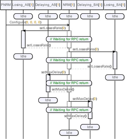
Figure 5.48 shows the sequence diagram resulting from the simulation of the medium configuration. Observe that the simulation corresponds to the results obtained in section 4.6.1.
The sequence diagram presented here is only an excerpt of the entire diagram, and focuses on our target simulation and the objects concerned. The detailed and extended diagrams are shown in Figure A.7 in the Appendix.
Figure 5.48. Simple transport protocol. Simulation: configuring the medium
5.7.2. No losses
Let us verify some of the already known scenarios. In this section, we will test how the simulation model reacts when there are no losses in the medium. For this, we will execute an open session request from User A without an answer from User B. Then we will again simulate the same scenario but, this second time, User B will accept the request.
5.7.2.1. Open session request without answer
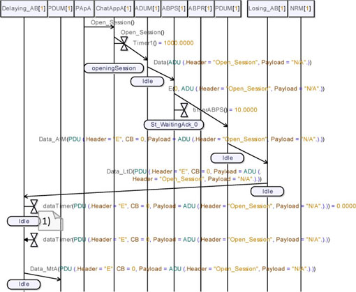
Note the first part of the sequence diagram obtained from simulation in Figure 5.49. The diagram shows the internal behavior of the Non-Reliable Medium (see note (1)), i.e. the packets exchanged between Losing_AB, Delaying_AB, Losing_BA and Delaying_BA classes. However, we tested this behavior in the last chapter and we are not interested in testing it again. Moreover, these lifelines might enlarge the resulting diagrams and complicate the reading.
Figure 5.49. Simple transport protocol. Simulation: no losses, open session req without answer (detailed)
We can run the simulation again. This time, we define the Non-Reliable Medium as a black-box, which means that we will not be able to see any of the interactions inside the NRM object. This new simulation allows us to focus on the protocol behavior.
Figure 5.50 shows the first part of this new simulation. Observe in note (1) that the chat application sets its internal timer to 1,000 time-units. Note also that the ADUM encapsulates the received packet and sends it forward to the ABPS (see note (2)). After that, the ABPS creates an E packet containing the received ADU; then, it sets its internal timer to 10 time-units. We can also note that the PDUM correctly creates a PDU describing the received packet (containing a header, a CB and an ADU) and forwards it to the NRM.
Figure 5.50. Simple transport protocol. Simulation: no losses, open session req without answer (Simplified 01)
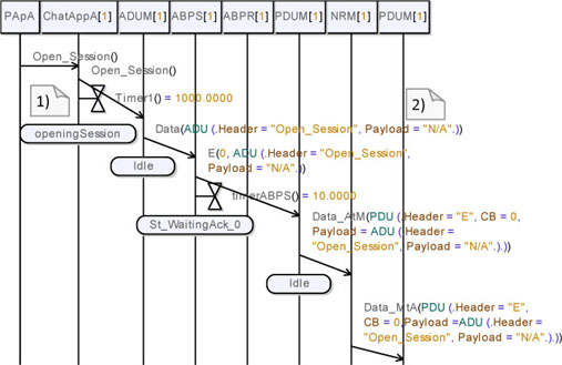
Figure 5.51 shows the continuation of the scenario. Observe, in note (1), that PDUM_B extracts the PDU from the received packet and forwards an E Packet to ABPR_B. ABPR_B acknowledges the received packet and forwards the received payload to the ADUM (see note (2)). Note also that the Open_Session packet correctly arrives to User B (represented here by PApB). Finally, note that the acknowledgement containing a CB equal to 0 correctly goes back and is received by ABPS_A (see note (3)).
We can now describe the state of the system at this point:
– first, ABPS_A knows that the packet was correctly received and it is waiting for a new data to transmit. It is in its St_WaitingData_1 state and has reset its internal timer;
– second, ChatAppB waits for an answer from its user and is in its waitingForAnswer state; and
– third, ChatAppA is in its openingSession state and waits for an answer from ChatAppB.
Figure 5.51. Simple transport protocol. Simulation: no losses, open session req without answer (Simplified 02)
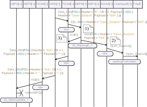
Figure 5.52. Simple transport protocol. Simulation: no losses, open session req without answer (Simplified 03)
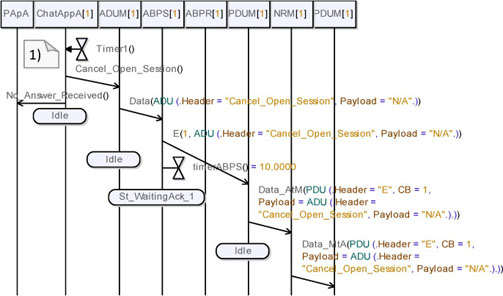
Figure 5.52 shows the continuation of this simulation.
We can observe in note (1) that ChatAppA’s internal timer is over. It then sends a Cancel_Open_Session and informs its user. The application packet is translated into an ADU and then into a PDU, and then sent to the medium.
Note in Figure 5.53 that the PDU is converted back into an ADU and into an application packet, and then delivered to ChatAppB. We can observe that a protocol-level acknowledgement containing a CB equal to 1 is sent back to ABPS_A. On receipt of this acknowledgement, ABPS_A resets its internal timer and goes to the St_WaitingData_0 state to wait for a new data to send.
Figure 5.53. Simple transport protocol. Simulation: no losses, open session req without answer (Simplified 04)
A detailed diagram of this simulation can be found in Figures A.8 and A.9 in the Appendix.
5.7.2.2. Open session request with answer
Figure 5.54. Simple transport protocol. Simulation: no losses, open session req with answer (01)

Figure 5.55. Simple transport protocol. Simulation: no losses, open session req with answer (02)

In Figure 5.54, we see that User A (represented here by PApA) sends a second Open_Session request. The sequence of messages shown in this diagram is the same as that in the previous simulation.
Then, in Figure 5.55 we can observe how the request is delivered to User B (represented here by PApB) and how the protocol-level acknowledgement is sent back to ABPS_A.
After this, User B accepts the session request, as shown in note (1) in Figure 5.56. In this figure, we can observe how the request is converted into an ADU, then into a PDU, then sent to the medium and finally delivered to the PDUM_A.
Figure 5.56. Simple transport protocol. Simulation: no losses, open session req with answer (03)
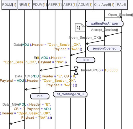
Figure 5.57 shows the session acknowledgement being delivered to ChatAppA. It also shows the protocol acknowledgement sent back by ABPR_A.
Figure 5.57. Simple transport protocol. Simulation: no losses, open session req with answer (04)
A detailed diagram of this simulation can be seen in Figure A.10 in the Appendix.
5.7.2.3. Send data
Let us suppose that the session is already established between the applications. Now, let us send a message from User A to User B and check what happens. Figure 5.58 shows the first part of the sequence diagram resulting from this simulation.
First, we can observe that all the objects in the diagram are in a stable state, i.e. no object is waiting for an answer.
Observe in note (1) (Figure 5.58) that User A (represented here by PApA) sends “Hello world” to his application. ChatAppA sends the received payload into the DataAP packet to the ADUM_A.
We can see that the packet is encapsulated into an ADU and then into a PDU. We can also observe that ABPS sets its internal timer to 10 time-units.
Figure 5.58. Simple transport protocol. Simulation: no losses, send data (01)
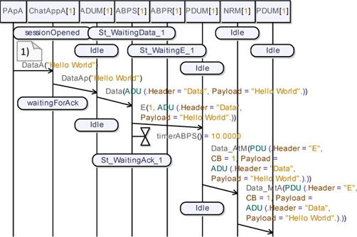
We can see in Figure 5.59 that the user message is correctly delivered to its destination and the protocol acknowledgement is sent back to ABPS.
Figure 5.59. Simple transport protocol. Simulation: no losses, send data (02)
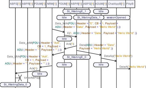
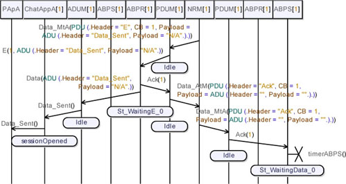
Figure 5.60 shows that ChatAppB delivers the user message to its destination and then sends a Data_Sent packet towards ChatAppA. We can see, again, how the packet passes through the transport protocol layer, then goes to the NRM and finally to the protocol layer.
Figure 5.60. Simple transport protocol. Simulation: no losses, send data (03)
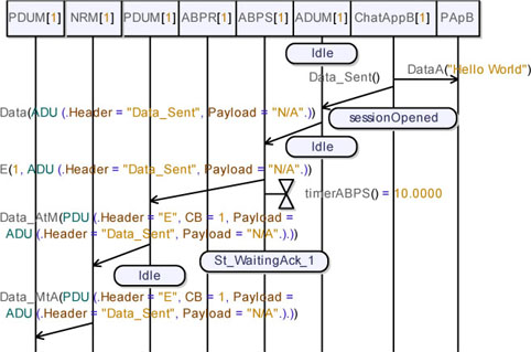
Figure 5.61. Simple transport protocol. Simulation: no losses, send data (04)
Finally, observe in Figure 5.61 how the application acknowledgements cross the protocol layer and then the application. Note that User A is informed by his application about the successful data transmission.
Finally, notice how the protocol acknowledgement is sent back and how the sender resets its internal timer.
A diagram containing the entire and detailed simulation of this scenario appears in Figure A.11 in the Appendix.
5.7.3. Losses
We can now test the recovery mechanisms implemented by the ABP. To do so, we will define a low reliability channel from A to B and a full reliability one from B to A.
We can test these conditions for a data transmission process. Remember that a data transmission from A to B is divided into two parts. In the first part, ChatAppA sends a data packet to B, while in the second part, ChatAppB answers with a Data_Sent packet. In the first part of the scenario we expect that, at protocol level, the E packet going from A to B will be lost by the medium and that the ABP modules will have to recover it. In the second part of the scenario, we expect that the protocol acknowledgement will be lost by the medium
For the moment we will not define any delay; however, in the next section, we will perform a simulation including some delay in the medium in order to illustrate how this ABP behaves under these circumstances.
Figure 5.62 shows the first part of this scenario. First, User A sends a data packet to his application, and the data packet contains the message “Hello World”. The Data packet is received by the application. Then it is forwarded to ADUM_A. After that, the application waits for an acknowledgement from ChatAppB.
The data packet arrives to ABPS_A. This module sends an E packet to PDUM_A; then it sets its internal timer and waits for an acknowledgement from ABPR_B.
Observe in note (1) that the medium loses the data packet. After some time, ABPS_A resends the data packet (see note (2)) and the medium loses the packet again. In the simulation that we perform, the packet is lost three times by the medium. However we will not show all the messages performing the resending operation in this section.
The entire and detailed sequence diagram is given in Figure A.12, Appendix.
Figure 5.62. Simple transport protocol. Simulation: losses, send data (01)
Observe in Figure 5.63 that ABPS resends the data packet and the medium delivers it to the receiver side. After that, the data packet is delivered to ABPR. Then, the message is sent to the chat application while a protocol acknowledgement is sent back to the sender.
Remember that we defined a full reliability from B to A; thus, the acknowledgement is delivered without problems, as expected. Note that, on receipt of the protocol acknowledgement, ABPS_A resets its internal timer and goes to the St_WaitingData_0 state and waits for a new data to transmit.
Figure 5.63. Simple transport protocol. Simulation: losses, send data (02)
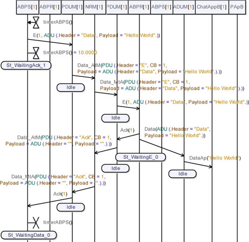
Figure 5.64 shows the instant when the data packet is delivered to ChatAppB. On receipt of the data packet, ChatAppB delivers it to its user and sends an acknowledgement packet to the sender application. Observe in note (1) that the packet correctly reaches the medium and then the PDUM_A.
In Figure 5.65 we can observe that the packet is delivered to ABPR_A. On receipt of the packet, ABPR_A sends an acknowledgement back to ABPS_B and sends the application acknowledgement towards ChatAppA. Observe in note (1) that the application receives the acknowledgement and informs its user. Note also that the protocol acknowledgement correctly reaches the medium, but it is not retransmitted (see note (2)).
Figure 5.64. Simple transport protocol. Simulation: losses, send data (03)
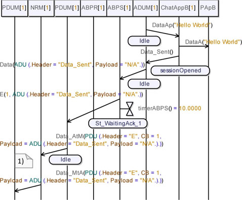
Figure 5.65. Simple transport protocol. Simulation: losses, send data (04)
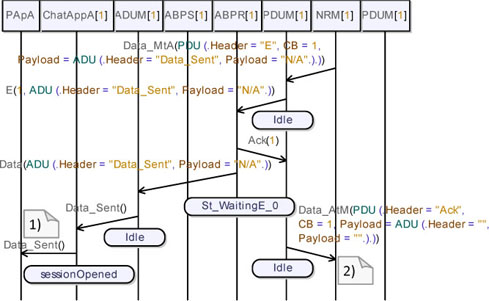
Figure 5.66 shows the moment where ABPS_B receives a timeout. On receipt of this signal, ABPS_B resends the data packet and waits for the protocol level acknowledgement.
Figure 5.66. Simple transport protocol. Simulation: losses, send data (05)
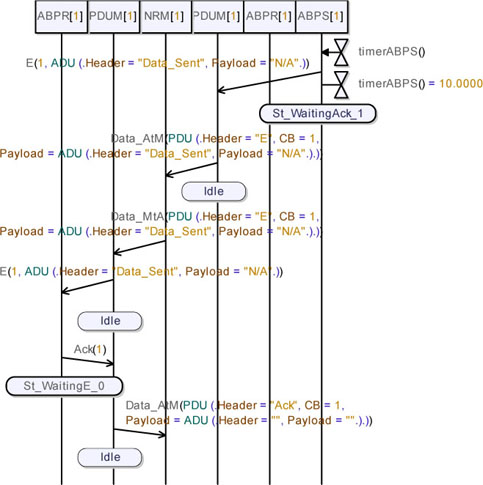
Again, the data packet is received by ABPR_A. This time, ABPR_A does not forward the packet towards the application since the received CB indicates that the packet was already received. Note that ABPR_A is waiting for a CB equal to 0, but the received CB is 1. Note also that the protocol acknowledgement correctly arrives at the medium, but it is not forwarded.
In this simulation, the protocol level acknowledgement was lost four times by the medium.
Not all the messages performing the resending operation are shown in this section. However, the entire and detailed sequence diagrams can be seen in Figures A.13 and A.14 in the Appendix.
Finally, Figure 5.67 shows that the protocol acknowledgement successfully goes back to ABPS_B. Again, note that, on receipt of the acknowledgement, ABPS_B resets its internal timer, and waits for a new data to transmit.
Figure 5.67. Simple transport protocol. Simulation: losses, send data (06)
This scenario allowed us to verify that our implementation of the Alternating Bit Protocol correctly transmits data packets over an unreliable network. It shows how the sender resends the data packets at regular intervals and how it manages the acknowledgements at different moments. It also shows how the receiver manages the repeated packets. It finally illustrates how the protocol behaves when either the E or the Ack packets are lost by the medium.
5.8. Further considerations
The Alternating Bit Protocol provides a reliable transport service on a non-reliable network. However, our current implementation of this algorithm cannot guarantee a reliable service when the network suffers from a high and variable delay. Indeed, the calculation of the timeout assigned to the protocol sender should mandatorily be set at least to the maximum round trip time; however, in our case, we set this timeout arbitrarily to 10 time units regardless of the maximum round trip time.
Let us now analyze two possible scenarios and observe how the protocol reacts under these circumstances.
5.8.1. Acknowledgements at different levels
The Simple Transport Protocol that we have modeled provides a reliable full duplex communication service to an application. This protocol implements the full duplex communication by duplicating the Alternating Bit unidirectional channel. As a consequence of this duplication, there is a separated channel for communicating from one point to another. This double channel at the protocol level may have an unexpected effect on applications. Indeed, the application-level data packets and the application-level acknowledgements travel on separate channels, and are then potentially submitted to different reliability and delay rates. Thus, an application level acknowledgement may arrive before a protocol level one.
We can imagine the following scenario:
– user A sends “Message 1” to his application;
– application A sends a data packet to Protocol A;
– protocol A sends an E packet to Protocol B;
– protocol B receives the data packet, then acknowledges the packet and forwards the payload to Application B;
– the acknowledgement sent by Protocol B is highly delayed by the medium;
– application B receives the data packet, then acknowledges the packet and forwards the payload to User B;
– the application-level acknowledgement sent by Application B arrives with no delay to Application A;
– user A sends “Message 2” to his application;
– application A sends a data packet to Protocol B;
– protocol B cannot receive a new data because it is still waiting for the delayed protocol-level acknowledgement. Thus, the data packet is lost;
– application A is blocked waiting for an acknowledgement from Application B.
Figure 5.68 briefly illustrates this scenario.
Figure 5.68. Simple transport protocol. Acknowledgement at different levels
It is possible to validate this scenario by simulation. Section A.2.4 in the Appendix shows a sequence diagram obtained by simulation. Figure A.18 (Appendix) shows the moment at which the data packet sent from application to protocol is lost.
We will not go into more detail about this simulation since the full validation of the protocol is not within the scope of this book. However, it is enough to say that a solution to this problem may consist of adding a buffer to the protocol sender in order to wait until the protocol is ready to process the received message.
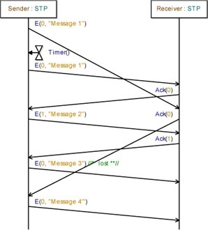
5.8.2. Delayed acknowledgements
Let us now imagine a situation where a highly delayed packet wrongly acknowledges another one. We can analyze the following scenario:
– Sender sends “message 1” to Receiver (E(CB=0));
– the packet is highly delayed by the network;
– the Sender considers the packets as lost since no answer is received (timeout);
– Sender resends “message 1’ to Receiver (CB = 0);
– Receiver receives “message 1” and acknowledges its receipt (CB = 0);
– Sender receives the acknowledgement with CB = 0 and sends “message 2’ to Receiver (CB = 1);
– Receiver receives the delayed “message 1” and acknowledges it (CB = 0). Acknowledgement with CB = 0 is highly delayed by the medium;
– Receiver receives “message 2” and acknowledges its receipt (CB = 1);
– Sender receives the acknowledgement with CB = 1 and sends “message 3’ to Receiver (CB = 0);
– “message 3” is lost by the network;
– Sender receives the delayed acknowledgement with CB = 0 and thinks that this is the acknowledgement of “message 3” (the last sent packet);
– Sender sends “message 4” to Receiver (CB = 1).
Note that “message 3” was lost by the medium but the sender does not realize it.
Figure 5.69 briefly illustrates this scenario.
The explanation of this problem is that the timeout assigned to the server is much shorter than the maximum delay experienced by a packet. We can solve this problem by incrementing the sender’s timeout. Indeed, the timeout assigned to the server must be at least a maximum round trip time.
A different solution to this problem consists of changing the range of the control header. Remember that the control header in the Alternating Bit protocol is called Control Bit, and it can only take values 0 or 1. By defining a larger control header (for example between 0 and 100), the protocol sender can ignore a very old acknowledgement.
It should be noted that several protocols and algorithms correctly deal with this kind of problem.
Figure 5.69. Simple transport protocol. Illustrating the limits of the ABP algorithm
5.9. Chapter summary
This chapter has concluded the book by linking all the preceding models together in one single model.
We have shown that it is possible to model different communication layers without using a particular programming language. This kind of analysis and design is usually called Model Driven Architecture (MDA).
We have shown in a practical way that MDA is highly enhanced by using Unified Modeling Language (UML).
All the examples presented in this book demonstrate that it is easily possible to model, analyze and test a communicating system by using an object-oriented approach. Of course, these examples do not pretend to undermine the traditional formal methods; on the contrary, our aim is to show some complementary tools which might greatly enhance the software development lifecycle.
The iterative and incremental design method used in this book needs to be underlined. This kind of approach is typically described by the Unified Process (UP). It encourages the division of a huge problem into small blocks. Each block is analyzed, conceived and implemented in a single iteration. Every iteration adds more complexity to the final model.
Finally, note that we used three different tools to create the models presented here. With the use of these tools, we can remark that the modeling language and the modeling process are independent from the software tools.
5.10. Bibliography
[DIA 09] DIAZ M. (ed.), Petri Nets, ISTE Ltd., London, John Wiley & Sons, New York, 2009.
1 Remember that a constructor in a class is a special type of subroutine called at the instantiation of an object. It prepares the new object for use, often accepting parameters which the constructor uses to set any attributes required when the object is first created.