350 Computer Architecture and Organization
operation of the process. We should remember that any process is executed in steps. Therefore, it
is frequently released from the processor before getting another chance to be executed again. As it
must restart from the same place it was terminated during its last execution, the value of the program
counter is always stored within the PCB when the process had to leave the processor halfway through
its execution.
11.2.4 Movements of a Process
The schematic presented in Figure 11.2 should not create the illusion that a process hops and jumps
from one point to another several times till the end of its execution. As a matter of fact, any process is
moved (copied to main memory from a disc) only once and till the end of its execution it stays at the
same location of the main memory. The movement from long-term to short-term queue is performed by
changing two related lists within the OS rather than physically shifting the program codes from one part
of memory to another. Similarly, the program counter of the processor is loaded with the current starting
memory address of the process to begin its execution and the program counter is loaded by the address
of the next process to stop the execution of the previous process. The I/O wait queue is also another list,
maintained by the OS, which may include and delete the process number as per the system requirement.
We should also note that all related details of the current phase are also stored within the process control
block for future use and reference.
11.3 SCHEDULING ISSUES
Scheduling is the term indicating the method to decide which process would be executed next by the
processor. The whole procedure of scheduling is overseen by the scheduler of the operating system. The
scheduler looks after or manages various queues, oversees that the processor and other resources are
properly utilized, and loads the processor at the appropriate moments with a selected process. Initially, it
does not seem to be a dif cult duty. Apparently, it is expected to maintain a few queues and by generat-
ing interrupts at regular intervals (depending upon the duration of the allotted time-slices to processes),
it needs to save the current program counter value within the PCB of the discarded process and load the
PC of the processor by the program counter value of the next process to be started. However, the matter
is more complex than that it seems to be, apparently.
11.3.1 CPU-bound and I/O-bound Processes
If we closely observe the programs executed by computers, we would conclude that they are one of the
two types CPU-bound or I/O-bound . A CPU-bound program needs more CPU time and its demand for I/O
time is negligible. On the other hand, an I/O-bound program demands more I/O time than the CPU time.
As example cases, we may consider two programs. The rst one is to solve a set of simultaneous equa-
tions and the second one is an on-screen animation program. Evidently, the rst program would keep the
CPU busy till it solved the problem and nally demand the I/O to display the results. On the other hand,
the animation program would keep on fetching and displaying graphics and would demand very less CPU
time. In our daily life, we rarely encounter any program that demands a balanced attention of CPU and I/O.
If the scheduler continues to send CPU-bound processes, then the I/O queue would remain almost
empty and the processor would be heavily loaded. Conversely, the CPU may remain idle and the I/O
M11_GHOS1557_01_SE_C11.indd 350M11_GHOS1557_01_SE_C11.indd 350 4/29/11 5:21 PM4/29/11 5:21 PM

Operating System 351
queue may be heavily populated if the scheduler continuously picks up I/O-bound processes. Techni-
cally speaking, the rst would be a CPU burst case and the next one would be the I/O burst case. We
have already indicated that one of the duties of OS is to optimize the usage of all available resources
of the computer. In the case of scheduling, it may only be achieved if a proper balance is maintained
between CPU-bound and I/O-bound processes. This has to be taken care of by the scheduler and it is
not an easy job.
11.3.2 Common Types of Scheduling
Within the long-term queue, a process spends (waits) more time giving the OS an ample scope to have a
rough idea about its system demands. At this stage, the OS shuf es the processes or keeps some tag on
them so that an appropriate process may be picked up for the short-term queue as soon as some process
is terminated, and, thus, generate a place for another. However, various other factors have created dif-
ferent type of scheduling and some of them are
R Shortest job rst (SJF)
R First come rst served (FCFS)
R Round robin scheduling (RR)
R Priority-based scheduling
Many of these methods may be either pre-emptive or non–pre-emptive. In the case of pre-emptive
scheduling, an ongoing process (process being executed by the processor) gets replaced by another pro-
cess of higher importance. This is not the case for non–pre-emptive scheduling. We shall discuss more
about it in following sections.
11.3.3 Efficiency of a Scheduling
To compare the ef ciency of different scheduling techniques, the parameter used as a practice is the
average waiting time. The waiting time of a process is the time it spends within the short-term queue,
waiting to be executed by the processor. The average waiting time is calculated by dividing the sum of
waiting time for all processes by the total number of processes involved.
The procedure becomes clearer if we consider some numerical examples. For this purpose, we
assume that there is no I/O wait involved. We consider only four processes with following parameters,
as presented in Table 11.1 .
Once in my class I was asked by a student whether any computer virus is CPU-bound or I/O-
bound. When the question was passed by me to other students, the only answer received was
‘CPU-bound’. Then I pointed it out that in some cases the display also suffers from the virus
attack and thus a balance was struck.
F
O
O
D
F
O
R
T
H
O
U
G
H
T
M11_GHOS1557_01_SE_C11.indd 351M11_GHOS1557_01_SE_C11.indd 351 4/29/11 5:21 PM4/29/11 5:21 PM
352 Computer Architecture and Organization
Process No.
Arrival time
(milliseconds)
CPU burst time
(milliseconds)
Priority
(if applicable) Remarks
P1 0 16 5
P2 10 12 3
P3 12 5 7 Lowest priority
P4 13 2 1 Highest priority
Table 11.1 Salient characteristics of four processes (Example case)
The arrival time is the time when a process arrives at the short-term queue. This parameter is in
milliseconds and the counting starts with the arrival time of the rst process, P1. CPU burst time is
the requirement of the total time of execution of the process, again in milliseconds. Priority is an
integer representation of the relative importance of a process for accessing the processor. Lower is
the integer value, higher is the priority. Using these parameters, we now explain following schedul-
ing techniques and calculate their average waiting time. Note that both waiting as well as execution
time are graphically represented for all techniques. However, the execution time is shaded while the
waiting time is not shaded in the following diagrams, to clearly distinguish between the two states of
the same process.
11.3.4 Non–pre-emptive SJF
As the name indicates, the process with shortest CPU-time-demand gets the privilege to be executed
earlier. Before allowing any new process to be executed, all available processes within the short term
queue are considered to pick-up the shortest one. As it is a case of non–pre-emptive SJF, once a process
has been allowed the processor-time, it would be allowed to be completely executed before the execu-
tion of the next selected process.
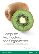
For the example problem, referring Table 11.1 , we nd that process 1 arrives rst and as no other
process is available, it is allowed to be executed immediately. Its execution (CPU burst time) takes
16 milliseconds and then the CPU is released by process 1. By this time three more processes are in
the short-term queue out of which P4 demands the shortest time (2 milliseconds). Therefore, process
P4 is allowed to be executed next. Then, it would be for process P3, requiring only 5 milliseconds.
Finally, process P2 was executed consuming 12 milliseconds of CPU time. The timeline of execution
of all four processes using non–pre-emptive SJF method is depicted in Figure 11.3 . We may now
calculate the waiting time for individual processes and then nd the average waiting time, which is
presented below.
Figure 11.3 Non–pre-emptive SJF
M11_GHOS1557_01_SE_C11.indd 352M11_GHOS1557_01_SE_C11.indd 352 4/29/11 5:21 PM4/29/11 5:21 PM
Operating System 353
Waiting time for process P1 = 0 millisecond
Waiting time for process P2 = 13 milliseconds
Waiting time for process P3 = 6 milliseconds
Waiting time for process P4 = 3 milliseconds
Total waiting time = 22 milliseconds
Average waiting time = 22/4 = 5.5 milliseconds
The guiding factors of scheduling by non–pre-emptive SJF method are
R The shortest among all available processes gets the priority.
R Once its execution starts, the process is never aborted.
11.3.5 Pre-emptive SJF
The major difference between non–pre-emptive SJF and pre-emptive SJF is the chance of taking away
an on-going process from the CPU if a process of shorter CPU-time-demand arrives. Note that the ongo-
ing process would not be aborted if the remaining time required to complete its execution is equal or less
than the just arrived process under consideration. To put it in another way, whenever any new process
arrives at the short term queue, its CPU-time-demand is compared with the remaining CPU time neces-
sary of the current process being executed.
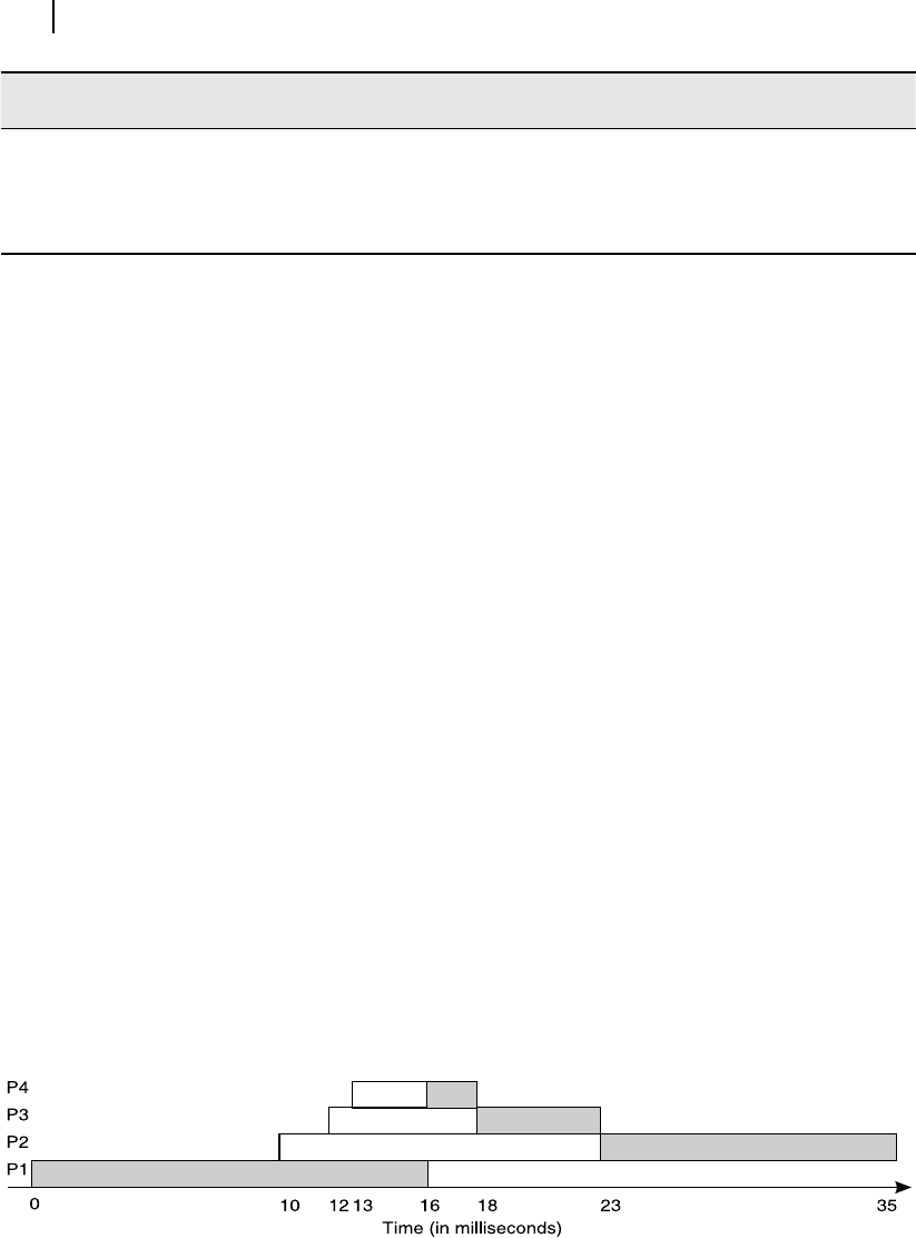
Considering our experimental data presented in Table 11.1 , we initiate our pre-emptive SJF with
Process 1, whose total CPU-time demand is 16 milliseconds. After its execution for 10 milliseconds,
Process 2 arrives, demanding a 12 milliseconds CPU-time. At this juncture, as Process 1 needs only 6
more milliseconds to complete its execution, Process 1 is not disturbed and is allowed to continue the
task. Process 3 arrives at 12 milliseconds needing 5 milliseconds for its completion and denied CPU
time as Process 1 needs only 4 milliseconds further, which is less than the demand of Process 3. Finally,
at the 13th millisecond, Process 4 arrives at the short-term queue needing only 2 milliseconds CPU-
time. As at this stage the ongoing process (Process 1) needs 3 milliseconds to complete itself, which is
more than the demand of Process 4, Process 1 is shifted out of the CPU and Process 4 is allowed to be
executed (Figure 10.4). Once Process 4 is completed, the turns come in the natural order to Process 1,
3 and 2, respectively, depending on their processor time requirements for completion. The timeline of
execution of all four processes (P1 – P4) using pre-emptive SJF technique is presented in Figure 11.4 .
The reader may compare it with Figure 11.3 and note the differences. The average waiting time may
now be calculated from individual waiting times, as follows:
Figure 11.4 Pre-emptive SJF
M11_GHOS1557_01_SE_C11.indd 353M11_GHOS1557_01_SE_C11.indd 353 4/29/11 5:22 PM4/29/11 5:22 PM

354 Computer Architecture and Organization
Waiting time for process P1 = 2 milliseconds
Waiting time for process P2 = 13 milliseconds
Waiting time for process P3 = 6 milliseconds
Waiting time for process P4 = 0 millisecond
Total waiting time = 21 milliseconds
Average waiting time = 21/4 = 5.25 milliseconds
Shortest job fi rst is a good method of scheduling. In case of pre-emptive SJF, the scheduler must
consider for eventual replacement of ongoing process immediately at the arrival of a new process.
11.3.6 First-Come-First-Served or FCFS
The next scheduling technique we should discuss is rst-come- rst-served or FCFS. As the name sug-
gests, the only order followed in this case is the order of arrival. FCFS is always non-pre-emptive,
unless we consider priority-based FCFS.
Figure 11.5 First-come-first-served or FCFS
Continuing with the same data set, schematic time-line of execution of the process is shown in
Figure 11.5 . In this case, P1 arrives rst and allowed the CPU time immediately. When P1 is nished
(after 16 milliseconds), by that time remaining three processes have arrived and obviously, the next
one in the queue, i.e., P2, is allowed the CPU time. Process P3 uses the processor next followed by
process P4. The average waiting time is calculated in usual manner, as follows:
Waiting time for process P1 = 0 millisecond
Waiting time for process P2 = 6 milliseconds
Waiting time for process P3 = 16 milliseconds
Waiting time for process P4 = 20 milliseconds
Total waiting time = 42 milliseconds
Average waiting time = 42/4 = 10.5 milliseconds
11.3.7 Round Robin
We now take up the Round Robin algorithm, whose main characteristic is to offer a prede ned time-
slice to every process. If the process is completed before the stipulated time, the next process in the
queue is allowed to use the CPU with a fresh (same duration) time-slice. However, if the process is not
M11_GHOS1557_01_SE_C11.indd 354M11_GHOS1557_01_SE_C11.indd 354 4/29/11 5:22 PM4/29/11 5:22 PM
..................Content has been hidden....................
You can't read the all page of ebook, please click here login for view all page.