Operating System 355
complete within its time-slice, it has to give room for the next process, and it is placed at the end of the
short-term queue.
For our data set, we assume a time-slice of 5 milliseconds and solve the scheduling problem with
that. If we assume a very large time-slice, say 100 milliseconds, then there would not be any difference
between this and FCFS method, for the assumed data set of Table 11.1 . Interested reader may try and
observe it.
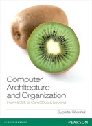
Figure 11.6 Round Robin (5 milliseconds time-slice)
So, we start our investigation with 5 milliseconds time-slice and remember that if any un nished pro-
cess is forced to leave the processor, it must be placed at the end of the queue, just like another new process.
To start with, process P1 enjoys two successive 5-millisecond time-slices as the next process, P2,
arrives at 10 milliseconds ( Figure 11.6 ). So, P1 leaves the CPU, occupying rst position of the queue as
P2 has now occupied the CPU for another 5 milliseconds. Note that total execution time of P1 and P2 are
16 and 12 milliseconds, respectively. However, during the execution of P2, P3 and P4 arrive and occupy
positions after P1 in the queue. Therefore, at the 15th millisecond, P2 releases the CPU and occupies
a position after P4 in the short-term queue. As P1 is rst in the short-term queue, it gets another 5 mil-
liseconds to use the processor.
After 20 milliseconds from starting, process P1 leaves the CPU and occupies the back seat of the
short-term queue behind P2. Note that P1 would need one more millisecond to complete its execution.
However, P3, in the now-leading position of the short-term queue, gets the chance for 5 milliseconds.
Thereafter, P4 occupies the CPU, for 2 milliseconds and next is the turn of P2. P2 gets another 5 milli-
seconds and leaves the CPU to make room of P1. Just after 1 millisecond, P1 completes its execution
and P2 gets its turn for completion of execution, which would now consume 2 milliseconds.
To calculate the average waiting time, we nd individual waiting time of all four processes, as fol-
lows (Figure 11.6 ):
Waiting time for process P1 = 17 milliseconds
Waiting time for process P2 = 13 milliseconds
Waiting time for process P3 = 8 milliseconds
Waiting time for process P4 = 12 milliseconds
Total waiting time = 50 milliseconds
Average waiting time = 50/4 = 12.5 milliseconds
11.3.8 Non–pre-emptive Priority
We shall now consider the fourth column of Table 11.1 in our scheduling experiments, which we have
ignored so far, as it was not necessary. This fourth column indicates the priority of the process, expressed
as an integer, and lesser is its value, higher would be the priority of the process. In pre-emptive priority
M11_GHOS1557_01_SE_C11.indd 355M11_GHOS1557_01_SE_C11.indd 355 4/29/11 5:22 PM4/29/11 5:22 PM
356 Computer Architecture and Organization
scheduling, the process with highest priority would occupy the CPU when it is free. Once a process has
occupied the CPU, even the arrival of a process with further higher priority would not be allowed to use
the CPU, till the ongoing process completes its execution. The idea is similar to SJF, with the difference
of not considering the burst-time but considering the assigned priority.
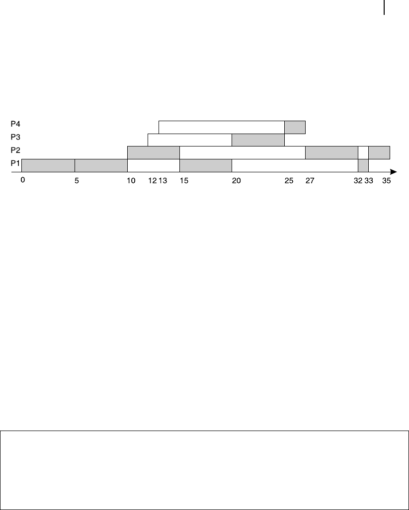
Figure 11.7 Non-pre-emptive priority
Referring Table 11.1 , the execution of process P1 starts and after 16 milliseconds, when it is n-
ished, we nd three processes waiting in the queue. The process with the highest priority is P4, which
is allowed the next CPU time. Priority-wise next turn goes to P2 and, nally, process P3 gets executed.
Figure 11.7 presents the related time-line and for an average waiting time calculation we proceed in the
same way as we have done it before.
Waiting time for process P1 = 0 milliseconds
Waiting time for process P2 = 8 milliseconds
Waiting time for process P3 = 18 milliseconds
Waiting time for process P4 = 3 milliseconds
Total waiting time = 29 milliseconds
Average waiting time = 29/4 = 7.25 milliseconds
11.3.9 Pre-emptive Priority
In pre-emptive priority based scheduling, arrival of a new process with higher priority would force an
ongoing process of lower priority to release the CPU. This may raise a question. As processes keep com-
ing within the short-term queue as long as the computer is active, would a process with a lowest priority
occupying the tail-end of the short-term queue or would it get any chance to be executed as priority?
If we strictly follow the rule of pre-emptive priority, then the answer is ‘no’. However, anticipating
this situation, generally, a technique is adopted to overcome this problem. After some prede ned time
intervals, e.g., 1 or 15 seconds, priority of all processes within the short-term queue are decremented
by one. Therefore, during the waiting stage, even a lowest priority process at the end of the queue
would earn the highest priority at some time-interval, and would get the processor time. This is known
as ageing .
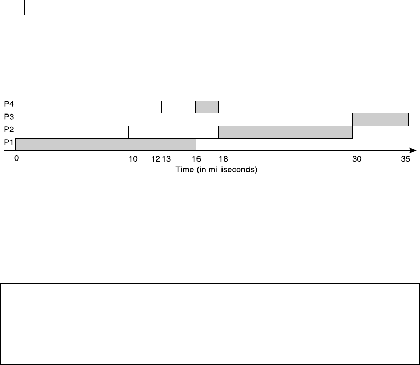
Continuing with our data set in Table 11.1 , we may foresee the time-line of execution of four
processes using pre-emptive priority scheduling method. It starts with process P1 as usual and after
10 milliseconds of its execution, it comes out of the CPU as P2 with higher priority arrives at that
time. However, at 13th millisecond, P2 is forced to make room for P4, which has even higher prior-
ity than P2.
M11_GHOS1557_01_SE_C11.indd 356M11_GHOS1557_01_SE_C11.indd 356 4/29/11 5:22 PM4/29/11 5:22 PM
Operating System 357
After completion of execution of P4, it may be observed that out of the three processes within the
short-term queue, P2 has the highest priority, and, therefore, gets the chance to use the processor rst.
Priority-wise next chance goes to process P1 and, nally, P3 with the lowest priority, is executed. The
time-line of this pre-emptive priority scheduling is presented in Figure 11.8 . The average waiting time
is calculated below.
Waiting time for process P1 = 14 milliseconds
Waiting time for process P2 = 2 milliseconds
Waiting time for process P3 = 18 milliseconds
Waiting time for process P4 = 0 millisecond
Total waiting time = 34 milliseconds
Average waiting time = 34/4 = 8.5 milliseconds
One important point may be noted by the reader at the end of this discussion about common schedul-
ing techniques. Although with our example data set, the minimum of average waiting time was secured
by the pre-emptive SJF method (5.25 milliseconds), it does not mean that this method is always found
to be optimum among all scheduling methods. As a matter of fact, the results we obtained are very much
dependent on the assumed data set (arrival time, CPU burst time, priority and time-slice).
11.3.10 Process Switching
The reader may be curious that, in case of Round Robin and other similar cases, how an ongoing process
is terminated at its midway of execution and another half-done process is resumed by the OS. How the
processor, which is under complete control of an ongoing process (set of instructions), would be under
the command of another process – the OS? The answer is, at no stage of any computer operation is the
system not under the control of the OS . It continuously monitors even an ongoing user-process and inter-
venes as and when felt necessary. The whole computer system, both its hardware as well as its software,
Figure 11.8 Pre-emptive priority
There are various types of scheduling and only a few are discussed in this section. Schedul-
ing is one of the important duties of an OS, specially in multi-tasking environment. Interested
readers may go through any textbook on OS for further information regarding these issues.
F
O
O
D
F
O
R
T
H
O
U
G
H
T
M11_GHOS1557_01_SE_C11.indd 357M11_GHOS1557_01_SE_C11.indd 357 4/29/11 5:22 PM4/29/11 5:22 PM
..................Content has been hidden....................
You can't read the all page of ebook, please click here login for view all page.