
6.5 Priority-Based Scheduling
The operating system’s fundamental job is to allocate resources in the computing system among programs that request them. Naturally, the CPU is the scarcest resource, so scheduling the CPU is the operating system’s most important job. In this section, we consider the structure of operating systems, how they schedule processes to meet performance requirements, and how they provide services beyond CPU scheduling.
Round-robin scheduling
A common scheduling algorithm in general-purpose operating systems is round-robin. All the processes are kept on a list and scheduled one after the other. This is generally combined with preemption so that one process does not grab all the CPU time. Round-robin scheduling provides a form of fairness in that all processes get a chance to execute. However, it does not guarantee the completion time of any task; as the number of processes increases, the response time of all the processes increases. Real-time systems, in contrast, require their notion of fairness to include timeliness and satisfaction of deadlines.
Process priorities
A common way to choose the next executing process in an RTOS is based on process priorities. Each process is assigned a priority, an integer-valued number. The next process to be chosen to execute is the process in the set of ready processes that has the highest-valued priority. Example 6.1 shows how priorities can be used to schedule processes.
Example 6.1 Priority-Driven Scheduling
For this example, we will adopt the following simple rules:
• Each process has a fixed priority that does not vary during the course of execution. (More sophisticated scheduling schemes do, in fact, change the priorities of processes to control what happens next.)
• The ready process with the highest priority (with 1 as the highest priority of all) is selected for execution.
• A process continues execution until it completes or it is preempted by a higher-priority process.
Let’s define a simple system with three processes as seen below.
| Process | Priority | Execution time |
| P1 | 1 | 10 |
| P2 | 2 | 30 |
| P3 | 3 | 20 |
In addition to describing the properties of the processes in general, we need to know the environmental setup. We assume that P2 is ready to run when the system is started, P1’s data arrive at time 15, and P3’s data arrive at time 18.
Once we know the process properties and the environment, we can use the priorities to determine which process is running throughout the complete execution of the system.
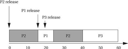
When the system begins execution, P2 is the only ready process, so it is selected for execution. At time 15, P1 becomes ready; it preempts P2 and begins execution because it has a higher priority. Because P1 is the highest-priority process in the system, it is guaranteed to execute until it finishes. P3’s data arrive at time 18, but it cannot preempt P1. Even when P1 finishes, P3 is not allowed to run. P2 is still ready and has higher priority than P3. Only after both P1 and P2 finish can P3 execute.
6.5.1 Rate-Monotonic Scheduling
Rate-monotonic scheduling (RMS), introduced by Liu and Layland [Liu73], was one of the first scheduling policies developed for real-time systems and is still very widely used. We say that RMS is a static scheduling policy because it assigns fixed priorities to processes. It turns out that these fixed priorities are sufficient to efficiently schedule the processes in many situations.
The theory underlying RMS is known as rate-monotonic analysis (RMA). This theory, as summarized below, uses a relatively simple model of the system.
• All processes run periodically on a single CPU.
• Context switching time is ignored.
• There are no data dependencies between processes.
• The execution time for a process is constant.
• All deadlines are at the ends of their periods.
• The highest-priority ready process is always selected for execution.
The major result of rate-monotonic analysis is that a relatively simple scheduling policy is optimal. Priorities are assigned by rank order of period, with the process with the shortest period being assigned the highest priority. This fixed-priority scheduling policy is the optimum assignment of static priorities to processes, in that it provides the highest CPU utilization while ensuring that all processes meet their deadlines. Example 6.2 illustrates rate-monotonic scheduling.
Example 6.2 Rate-Monotonic Scheduling
Here is a simple set of processes and their characteristics.
| Process | Execution time | Period |
| P1 | 1 | 4 |
| P2 | 2 | 6 |
| P3 | 3 | 12 |
Applying the principles of RMA, we give P1 the highest priority, P2 the middle priority, and P3 the lowest priority. To understand all the interactions between the periods, we need to construct a timeline equal in length to the least-common multiple of the process periods, which is 12 in this case. The complete schedule for the least-common multiple of the periods is called the unrolled schedule.
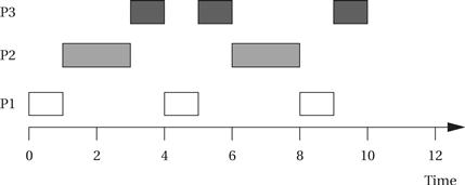
All three periods start at time zero. P1’s data arrive first. Because P1 is the highest-priority process, it can start to execute immediately. After one time unit, P1 finishes and goes out of the ready state until the start of its next period. At time 1, P2 starts executing as the highest-priority ready process. At time 3, P2 finishes and P3 starts executing. P1’s next iteration starts at time 4, at which point it interrupts P3. P3 gets one more time unit of execution between the second iterations of P1 and P2, but P3 doesn’t get to finish until after the third iteration of P1.
Consider the following different set of execution times for these processes, keeping the same deadlines.
| Process | Execution time | Period |
| P1 | 2 | 4 |
| P2 | 3 | 6 |
| P3 | 3 | 12 |
In this case, we can show that there is no feasible assignment of priorities that guarantees scheduling. Even though each process alone has an execution time significantly less than its period, combinations of processes can require more than 100% of the available CPU cycles. For example, during one 12 time-unit interval, we must execute P1 three times, requiring 6 units of CPU time; P2 twice, costing 6 units of CPU time; and P3 one time, requiring 3 units of CPU time. The total of 6 + 6 + 3 = 15 units of CPU time is more than the 12 time units available, clearly exceeding the available CPU capacity.
Liu and Layland [Liu73] proved that the RMA priority assignment is optimal using critical-instant analysis. We define the response time of a process as the time at which the process finishes. The critical instant for a process is defined as the instant during execution at which the task has the largest response time. It is easy to prove that the critical instant for any process P, under the RMA model, occurs when it is ready and all higher-priority processes are also ready—if we change any higher-priority process to waiting, then P’s response time can only go down.
We can use critical-instant analysis to determine whether there is any feasible schedule for the system. In the case of the second set of execution times in, there was no feasible schedule. Critical-instant analysis also implies that priorities should be assigned in order of periods. Let the periods and computation times of two processes P1 and P2 be τ1, τ2 and T1, T2, with τ1< τ2. We can generalize the result of Example 6.2 to show the total CPU requirements for the two processes in two cases. In the first case, let P1 have the higher priority. In the worst case we then execute P2 once during its period and as many iterations of P1 as fit in the same interval. Because there are ![]() iterations of P1 during a single period of P2, the required constraint on CPU time, ignoring context switching overhead, is
iterations of P1 during a single period of P2, the required constraint on CPU time, ignoring context switching overhead, is
 (Eq. 6.2)
If, on the other hand, we give higher priority to P2, then critical-instant analysis tells us that we must execute all of P2 and all of P1 in one of P1’s periods in the worst case:
![]() (Eq. 6.3)
(Eq. 6.3)
There are cases where the first relationship can be satisfied and the second cannot, but there are no cases where the second relationship can be satisfied and the first cannot. We can inductively show that the process with the shorter period should always be given higher priority for process sets of arbitrary size. It is also possible to prove that RMS always provides a feasible schedule if such a schedule exists.
CPU utilization
The bad news is that, although RMS is the optimal static-priority schedule, it does not allow the system to use 100% of the available CPU cycles. The total CPU utilization for a set of n tasks is
 (Eq. 6.4)
It is possible to show that for a set of two tasks under RMS scheduling, the CPU utilization U will be no greater than 2(21/2 − 1) ≅ 0.83. In other words, the CPU will be idle at least 17% of the time. This idle time is due to the fact that priorities are assigned statically; we see in the next section that more aggressive scheduling policies can improve CPU utilization. When there are m tasks, the maximum processor utilization is
![]() (Eq. 6.5)
(Eq. 6.5)
As m approaches infinity, the CPU utilization asymptotically approaches ln 2 = 0.69—the CPU will be idle 31% of the time. We can use processor utilization U as an easy measure of the feasibility of an RMS scheduling problem.
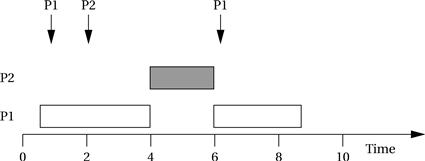
Figure 6.11 shows an example of an RMS schedule for a system in which P1 has a period of 4 and an execution time of 2 and P2 has a period of 12 and an execution time of 1. The execution of P2 is preempted by P1 during P2’s first period and P2’s second. The least-common multiple of the periods of the processes is 12, so the CPU utilization of this set of processes is [(2 × 3) + (1 × 12)]/12 = 0.58333, which is within the feasible utilization of RMS.
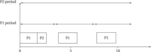
Figure 6.11 An example of rate-monotonic scheduling.
Implementation
The implementation of RMS is very simple. Figure 6.12 shows C code for an RMS scheduler run at the operating system’s timer interrupt. The code merely scans through the list of processes in priority order and selects the highest-priority ready process to run. Because the priorities are static, the processes can be sorted by priority in advance before the system starts executing. As a result, this scheduler has an asymptotic complexity of O(n), where n is the number of processes in the system. (This code assumes that processes are not created dynamically. If dynamic process creation is required, the array can be replaced by a linked list of processes, but the asymptotic complexity remains the same.) The RMS scheduler has both low asymptotic complexity and low actual execution time, which helps minimize the discrepancies between the zero-context-switch assumption of rate-monotonic analysis and the actual execution of an RMS system.
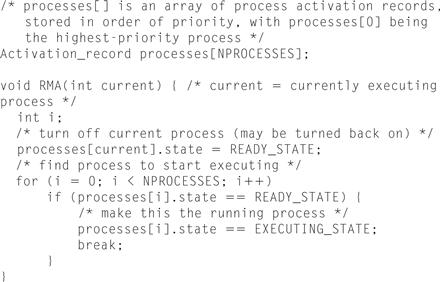
Figure 6.12 C code for rate-monotonic scheduling.
6.5.2 Shared Resources
A process may need to do more than read and write values memory. For example, it may need to communicate with an I/O device. And it may use shared memory locations to communicate with other processes. When dealing with shared resources special care must be taken.
Race condition
Consider the case in which an I/O device has a flag that must be tested and modified by a process. Problems can arise when other processes may also want to access the device. If combinations of events from the two tasks operate on the device in the wrong order, we may create a critical timing race or race condition that causes erroneous operation. For example:
1. Task 1 reads the flag location and sees that it is 0.
2. Task 2 reads the flag location and sees that it is 0.
3. Task 1 sets the flag location to 1 and writes data to the I/O device’s data register.
4. Task 2 also sets the flag to 1 and writes its own data to the device data register, overwriting the data from task 1.
In this case, both devices thought they were able to write to the device, but the task 1’s write was never completed because it was overridden by task 2.
Critical sections
To prevent this type of problem we need to control the order in which some operations occur. For example, we need to be sure that a task finishes an I/O operation before allowing another task to starts its own operation on that I/O device. We do so by enclosing sensitive sections of code in a critical section that executes without interruption.
Semaphores
We create a critical section using semaphores, which are a primitive provided by the operating system. The semaphore is used to guard a resource. (The term semaphore was derived from railroads, in which a shared section of track is guarded by signal flags that use semaphores to signal when it is safe to enter the track.) We start a critical section by calling a semaphore function that does not return until the resource is available. When we are done with the resource we use another semaphore function to release it. The semaphore names are, by tradition, P() to gain access to the protected resource and V() to release it.
/* some nonprotected operations here */
P(); /* wait for semaphore */
/* do protected work here */
V(); /* release semaphore */
This form of semaphore assumes that all system resources are guarded by the same P()/V() pair. Many operating systems also provide named resources that allow different resources to be grouped together. A call to P() or V() provides a resource name argument. Calls that refer to different resources may execute concurrently. Many operating systems also provide counting semaphores so that, for example, up to n tasks may pass the P() at any given time. If more tasks want to enter, they will wait until a task has released the resource.
Test-and-set
To implement P() and V(), the microprocessor bus must support an atomic read/write operation, which is available on a number of microprocessors. These types of instructions first read a location and then set it to a specified value, returning the result of the test. If the location was already set, then the additional set has no effect but the instruction returns a false result. If the location was not set, the instruction returns true and the location is in fact set. The bus supports this as an atomic operation that cannot be interrupted.
Programming Example 6.2 describes the ARM atomic read/write operation in more detail.
Programming Example 6.2 Compare-and-Swap Operations
The SWP (swap) instruction is used in the ARM to implement atomic compare-and-swap:
SWP Rd,Rm,Rn
The SWP instruction takes three operands—the memory location pointed to by Rn is loaded and saved into Rd, and the value of Rm is then written into the location pointed to by Rn. When Rd and Rn are the same register, the instruction swaps the register’s value and the value stored at the address pointed to by Rd/Rn. For example, the code sequence
ADR r0, SEMAPHORE ; get semaphore address
LDR r1, #1
GETFLAG SWP r1,r1,[r0] ; test-and-set the flag
BNZ GETFLAG ; no flag yet, try again
HASFLAG …
first loads the constant 1 into r1 and the address of the semaphore FLAG1 into register r2, then reads the semaphore into r0 and writes the 1 value into the semaphore. The code then tests whether the semaphore fetched from memory is zero; if it was, the semaphore was not busy and we can enter the critical region that begins with the HASFLAG label. If the flag was nonzero, we loop back to try to get the flag once again.
The test-and-set allows us to implement semaphores. The P() operation uses a test-and-set to repeatedly test a location that holds a lock on the memory block. The P() operation does not exit until the lock is available; once it is available, the test-and-set automatically sets the lock. Once past the P() operation, the process can work on the protected memory block. The V() operation resets the lock, allowing other processes access to the region by using the P() function.
Critical sections and timing
Critical sections pose some problems for real-time systems. Because the interrupt system is shut off during the critical section, the timer cannot interrupt and other processes cannot start to execute. The kernel may also have its own critical sections that keep interrupts from being serviced and other processes from executing.
6.5.3 Priority Inversion
Shared resources cause a new and subtle scheduling problem: a low-priority process blocks execution of a higher-priority process by keeping hold of its resource, a phenomenon known as priority inversion. Example 6.3 illustrates the problem.
Example 6.3 Priority Inversion
A system with three processes: P1 has the highest priority, P3 has the lowest priority, and P2 has a priority in between that of P1 and P3. P1 and P3 both use the same shared resource. Processes become ready in this order:
*P3 becomes ready and enters its critical region, reserving the shared resource.
*P2 becomes ready and preempts P3.
*P1 becomes ready. It will preempt P2 and start to run but only until it reaches its critical section for the shared resource. At that point, it will stop executing.
For P1 to continue, P2 must completely finish, allowing P3 to resume and finish its critical section. Only when P3 is finished with its critical section can P1 resume.
Priority inheritance
The most common method for dealing with priority inversion is priority inheritance: promote the priority of any process when it requests a resource from the operating system. The priority of the process temporarily becomes higher than that of any other process that may use the resource. This ensures that the process will continue executing once it has the resource so that it can finish its work with the resource, return it to the operating system, and allow other processes to use it. Once the process is finished with the resource, its priority is demoted to its normal value.
6.5.4 Earliest-Deadline-First Scheduling
Earliest deadline first (EDF) is another well-known scheduling policy that was also studied by Liu and Layland [Liu73]. It is a dynamic priority scheme—it changes process priorities during execution based on initiation times. As a result, it can achieve higher CPU utilizations than RMS.
The EDF policy is also very simple: It assigns priorities in order of deadline. The highest-priority process is the one whose deadline is nearest in time, and the lowest-priority process is the one whose deadline is farthest away. Clearly, priorities must be recalculated at every completion of a process. However, the final step of the OS during the scheduling procedure is the same as for RMS—the highest-priority ready process is chosen for execution.
Example 6.4 illustrates EDF scheduling in practice.
Example 6.4 Earliest-Deadline-First Scheduling
Consider the following processes:
| Process | Execution time | Period |
| P1 | 1 | 3 |
| P2 | 1 | 4 |
| P3 | 2 | 5 |
The least-common multiple of the periods is 60, and the utilization is 1/3 + 1/4 + 1/5 = 0.9833333. This utilization is too high for RMS, but it can be handled with an earliest-deadline-first schedule. Here is the schedule:
| Time | Running process | Deadlines |
| 0 | P1 | |
| 1 | P2 | |
| 2 | P3 | P1 |
| 3 | P3 | P2 |
| 4 | P1 | P3 |
| 5 | P2 | P1 |
| 6 | P1 | |
| 7 | P3 | P2 |
| 8 | P3 | P1 |
| 9 | P1 | P3 |
| 10 | P2 | |
| 11 | P3 | P1, P2 |
| 12 | P3 | |
| 13 | P1 | |
| 14 | P2 | P1, P3 |
| 15 | P1 | P2 |
| 16 | P2 | |
| 17 | P3 | P1 |
| 18 | P3 | |
| 19 | P1 | P2, P3 |
| 20 | P2 | P1 |
| 21 | P1 | |
| 22 | P3 | |
| 23 | P3 | P1, P2 |
| 24 | P1 | P3 |
| 25 | P2 | |
| 26 | P3 | P1 |
| 27 | P3 | P2 |
| 28 | P1 | |
| 29 | P2 | P1, P3 |
| 30 | P1 | |
| 31 | P3 | P2 |
| 32 | P3 | P1 |
| 33 | P1 | |
| 34 | P2 | P3 |
| 35 | P3 | P1, P2 |
| 36 | P1 | |
| 37 | P2 | |
| 38 | P3 | P1 |
| 39 | P1 | P2, P3 |
| 40 | P2 | |
| 41 | P3 | P1 |
| 42 | P1 | |
| 43 | P3 | P2 |
| 44 | P3 | P1, P3 |
| 45 | P1 | |
| 46 | P2 | |
| 47 | P3 | P1, P2 |
| 48 | P3 | |
| 49 | P1 | P3 |
| 50 | P2 | P1 |
| 51 | P1 | P2 |
| 52 | P3 | |
| 53 | P3 | P1 |
| 54 | P2 | P3 |
| 55 | P1 | P2 |
| 56 | P2 | P1 |
| 57 | P3 | |
| 58 | P3 | |
| 59 | idle | P1, P2, P3 |
There is one time slot left at the end of this unrolled schedule, which is consistent with our earlier calculation that the CPU utilization is 59/60.
Liu and Layland showed that EDF can achieve 100% utilization. A feasible schedule exists if the CPU utilization (calculated in the same way as for RMA) is less than or equal to 1. They also showed that when an EDF system is overloaded and misses a deadline, it will run at 100% capacity for a time before the deadline is missed. Distinguishing between a system that is running just at capacity and one that is about to miss a deadline is difficult, making the use of very high deadlines problematic.
The implementation of EDF is more complex than the RMS code. Figure 6.13 outlines one way to implement EDF. The major problem is keeping the processes sorted by time to deadline—because the times to deadlines for the processes change during execution, we cannot presort the processes into an array, as we could for RMS. To avoid re-sorting the entire set of records at every change, we can build a binary tree to keep the sorted records and incrementally update the sort. At the end of each period, we can move the record to its new place in the sorted list by deleting it from the tree and then adding it back to the tree using standard tree manipulation techniques. We must update process priorities by traversing them in sorted order, so the incremental sorting routines must also update the linked list pointers that let us traverse the records in deadline order. (The linked list lets us avoid traversing the tree to go from one node to another, which would require more time.) After putting in the effort to building the sorted list of records, selecting the next executing process is done in a manner similar to that of RMS. However, the dynamic sorting adds complexity to the entire scheduling process. Each update of the sorted list requires O(n log n) steps. The EDF code is also significantly more complex than the RMS code.
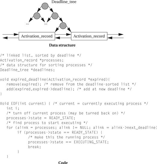
Figure 6.13 C code for earliest-deadline-first scheduling.
6.5.7 RMS versus EDF
Which scheduling policy is better: RMS or EDF? That depends on your criteria. EDF can extract higher utilization out of the CPU, but it may be difficult to diagnose the possibility of an imminent overload. Because the scheduler does take some overhead to make scheduling decisions, a factor that is ignored in the schedulability analysis of both EDF and RMS, running a scheduler at very high utilizations is somewhat problematic. RMS achieves lower CPU utilization but is easier to ensure that all deadlines will be satisfied. In some applications, it may be acceptable for some processes to occasionally miss deadlines. For example, a set-top box for video decoding is not a safety-critical application, and the occasional display artifacts caused by missing deadlines may be acceptable in some markets.
What if your set of processes is unschedulable and you need to guarantee that they complete their deadlines? There are several possible ways to solve this problem:
• Get a faster CPU. That will reduce execution times without changing the periods, giving you lower utilization. This will require you to redesign the hardware, but this is often feasible because you are rarely using the fastest CPU available.
• Redesign the processes to take less execution time. This requires knowledge of the code and may or may not be possible.
• Rewrite the specification to change the deadlines. This is unlikely to be feasible, but may be in a few cases where some of the deadlines were initially made tighter than necessary.
6.5.8 A Closer Look at Our Modeling Assumptions
Our analyses of RMS and EDF have made some strong assumptions. These assumptions have made the analyses much more tractable, but the predictions of analysis may not hold up in practice. Because a misprediction may cause a system to miss a critical deadline, it is important to at least understand the consequences of these assumptions.
Rate-monotonic scheduling assumes that there are no data dependencies between processes. Example 6.5 shows that knowledge of data dependencies can help use the CPU more efficiently.
Example 6.5 Data Dependencies and Scheduling
Data dependencies imply that certain combinations of processes can never occur. Consider the simple example [Mal96] below.

We know that P1 and P2 cannot execute at the same time, because P1 must finish before P2 can begin. Furthermore, we also know that because P3 has a higher priority, it will not preempt both P1 and P2 in a single iteration. If P3 preempts P1, then P3 will complete before P2 begins; if P3 preempts P2, then it will not interfere with P1 in that iteration. Because we know that some combinations of processes cannot be ready at the same time, we know that our worst-case CPU requirements are less than would be required if all processes could be ready simultaneously.
One important simplification we have made is that contexts can be switched in zero time. On the one hand, this is clearly wrong—we must execute instructions to save and restore context, and we must execute additional instructions to implement the scheduling policy. On the other hand, context switching can be implemented efficiently—context switching need not kill performance. The effects of nonzero context switching time must be carefully analyzed in the context of a particular implementation to be sure that the predictions of an ideal scheduling policy are sufficiently accurate. Example 6.6 shows that context switching can, in fact, cause a system to miss a deadline.
Example 6.6 Scheduling and Context Switching Overhead
Appearing below is a set of processes and their characteristics.
| Process | Execution time | Deadline |
| P1 | 3 | 5 |
| P2 | 3 | 10 |
First, let us try to find a schedule assuming that context switching time is zero. Following is a feasible schedule for a sequence of data arrivals that meets all the deadlines:
Now let us assume that the total time to initiate a process, including context switching and scheduling policy evaluation, is one time unit. It is easy to see that there is no feasible schedule for the above data arrival sequence, because we require a total of 2TP 1 + TP 2 = 2 × (1 + 3) + (1 + 3) = 11 time units to execute one period of P2 and two periods of P1.
In most real-time operating systems, a context switch requires only a few hundred instructions, with only slightly more overhead for a simple real-time scheduler like RMS. These small overhead times are not likely to cause serious scheduling problems. Problems are most likely to manifest themselves in the highest-rate processes, which are often the most critical in any case. Completely checking that all deadlines will be met with nonzero context switching time requires checking all possible schedules for processes and including the context switch time at each preemption or process initiation. However, assuming an average number of context switches per process and computing CPU utilization can provide at least an estimate of how close the system is to CPU capacity.
Rhodes and Wolf [Rho97] developed a CAD algorithm for implementing processes that computes exact schedules to accurately predict the effects of context switching. Their algorithm selects between interrupt-driven and polled implementations for processes on a microprocessor. Polled processes introduce less overhead, but they do not respond to events as quickly as interrupt-driven processes. Furthermore, because adding interrupt levels to a microprocessor usually incurs some cost in added logic, we do not want to use interrupt-driven processes when they are not necessary. Their algorithm computes exact schedules for the processes, including the overhead for polling or interrupts as appropriate, and then uses heuristics to select implementations for the processes. The major heuristic starts with all processes implemented as polled mode, and then changes processes that miss deadlines to use interrupts. Some iterative improvement steps try various combinations of interrupt-driven processes to eliminate deadline violations. These heuristics minimize the number of processes implemented with interrupts.
Another important assumption we have made thus far is that process execution time is constant. As seen in Section 5.6, this is definitely not the case—both data-dependent behavior and caching effects can cause large variations in run times. The techniques for bounding the cache-based performance of a single program do not work when multiple programs are in the same cache. The state of the cache depends on the product of the states of all programs executing in the cache, making the state space of the multiple-process system exponentially larger than that for a single program. We discuss this problem in more detail in 6.7.