
The programs we have developed in the previous chapters of this book are not explicitly concerned with the passage of time. We have used delays to make the execution of example programs viewable in a convenient way, however the correct operation of these programs is independent of time. Correctness depends on performing actions in a certain order and not on performing an action by a certain time. This has the advantage that the programs work safely, independently of processor speed and thread scheduling.
In this chapter, we develop programs that are concerned with the passage of time and in which correctness does depend on performing actions by specific times. In general, we deal with the relationship between the time at which program actions are executed and the time that events occur in the real world. We make the simplifying assumption that program execution proceeds sufficiently quickly such that, when related to the time between external events, it can be ignored. For example, consider a program that detects double mouse clicks. The program notes the time that passes between successive mouse clicks and causes a double-click action to be executed when this is less than some specified period. The inter-click time for such a program would be specified in tenths of a second, while the instructions necessary to recognize clicks and measure the inter-click time would require tenths of a millisecond. In modeling and developing such a program, it is reasonable to ignore the execution time of actions. We can assume that the execution of an action takes zero time, although we do not assume that executing an infinite number of actions takes zero time. A much more difficult approach to action execution time is to specify and subsequently guarantee an upper bound to execution time. This falls into a specialized area of concurrent software design termed real-time and it is beyond the scope of this book.
In the following, we first examine how we can incorporate time into models and then how the behavior exhibited by these models can be implemented in Java.
In Chapter 3, we stated that our model of concurrent execution was asynchronous; processes proceed at arbitrary relative speeds. Consequently, the delay between two successive actions of a process can take an arbitrarily long time. How then do we make processes aware of the passage of time and, in particular, how can we synchronize their execution with time? The answer is to adopt a discrete model of time in which the passage of time is signaled by successive ticks of a clock. Processes become aware of the passage of time by sharing a global tick action. Time is measured as a positive integer value. To illustrate the use of this model of time, we return to the double-click program described in the introduction to the chapter. Figure 12.1 depicts the relationship between discrete time and mouse clicks.
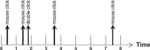
To make the discussion concrete, assume that the unit of time represented in Figure 12.1 is a second. We specify that a double-click should be recognized when the time between two successive mouse clicks is less than, say, three seconds. We can easily see that the click during period 0 and the click during period 1 constitute a double-click since the interval between these clicks must be less than two seconds. The click during period 3 and the click during period 7 do not form a double-click since there is an interval between these clicks of at least three seconds. The use of discrete time means that we cannot determine precisely when an event occurs, we can only say that it occurs within some period delimited by two ticks of the clock. This gives rise to some timing uncertainty. For example, if the last mouse click happened in period 6, would a double-click have occurred or not? The most we could say is that the last two mouse clicks were separated by at least two seconds and not more than four seconds. We can increase the accuracy by having more ticks per second, however some uncertainty remains. For example, with two ticks per second, we could say that two clicks were separated by at least 2.5 seconds and not more than 3.5 seconds. In fact, this uncertainty also exists in implementations since time is measured in computer systems using a clock that ticks with a fixed periodicity, usually in the order of milliseconds. An implementation can only detect that two events are separated by time (n ± 1) * T, where T is the periodicity of the clock and n the number of clock ticks between the two events. In general, despite the limitations we have discussed above, discrete time is sufficient to model many timed systems since it is also the way time is represented in implementations.
In the example above, if we want to ensure that the clicks which form a double-click are never more than three seconds apart, the last click would have to happen in period 5. Consequently, after the first mouse click occurs, the clock must not tick more than two times before the second click of a double-click occurs. To capture the behavior of the double-click program as a model in FSP, we use the tick action to signal the beginning (and end) of each period. A doubleclick action occurs if less than three tick actions occur between successive mouse clicks. The behavior of the double-click program is modeled as follows:
DOUBLECLICK(D=3) =
(tick -> DOUBLECLICK | click -> PERIOD[1]),
PERIOD[t:1..D] =
(when (t==D) tick -> DOUBLECLICK
|when (t<D) tick -> PERIOD[t+1]
|click -> doubleclick -> DOUBLECLICK
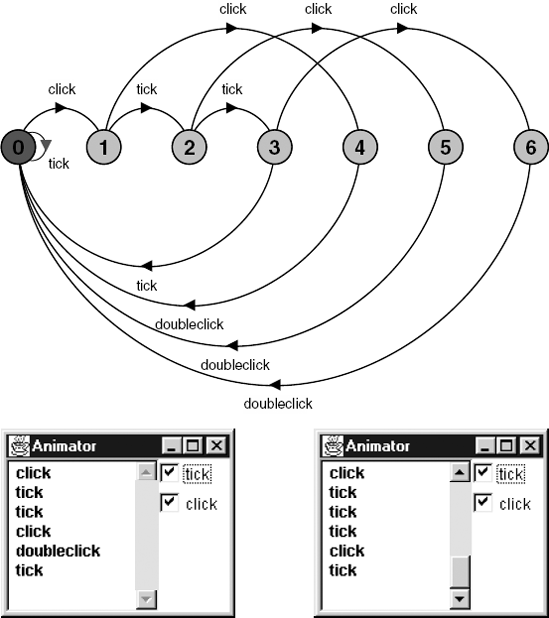
).The DOUBLECLICK process accepts a click action at any time, since, initially, there is a choice between click and tick. When a click occurs, the process starts counting the tick s that follow. If a click occurs before the third succeeding tick, then a doubleclick action is output, otherwise the process resets. Figure 12.2 shows the LTS for DOUBLECLICK and two possible traces of the model; in (a) a doubleclick is output after two clicks and in (b) it is not.
In discussing the double-click program, we assumed that clock ticks occur every second. However, this is simply an interpretation of the model. We choose an interpretation for a tick that is appropriate to the problem at hand. For example, in modeling hardware circuits, ticks would delimit periods measured in nanoseconds. However, within a particular time frame, the more accurately we represent time, the larger the model. For example, if we wanted to increase the accuracy of the double-click model while retaining the same time frame, we could decide to have two ticks per second and, consequently, the parameter D would become 6 rather than 3. This would double the number of states in DOUBLECLICK.
The previous example dealt with how a process is made aware of the passage of time. We now examine the implications of time in models with multiple processes. We look at a simple producer – consumer system in which the PRODUCER process produces an item every Tp seconds and the CONSUMER process takes Tc seconds to consume an item. The models for the PRODUCER and CONSUMER processes are listed below:
CONSUMER(Tc=3) =
       (item -> DELAY[1] | tick -> CONSUMER),
     DELAY[t:1..Tc] =
       (when(t==Tc) tick -> CONSUMER
       |when(t<Tc)  tick -> DELAY[t+1]
       ).

     PRODUCER(Tp=3) =
       (item -> DELAY[1]),
     DELAY[t:1..Tp] =
       (when(t==Tp) tick -> PRODUCER
       |when(t<Tp)  tick -> DELAY[t+1]
       ).
Note that the consumer initially has a choice between getting an item and a tick action. This models waiting for an action to happen while allowing time to pass. We can model the three possible situations that can occur when the PRODUCER and CONSUMER processes are combined. Firstly, the situation where items are produced at the same rate that they are consumed:
||SAME = (PRODUCER(2) || CONSUMER(2)).
Analysis of this system does not detect any safety problems. Similarly, analysis detects no problems in the system in which items are produced at a slower rate that they are consumed:
||SLOWER = (PRODUCER(3) || CONSUMER(2)).
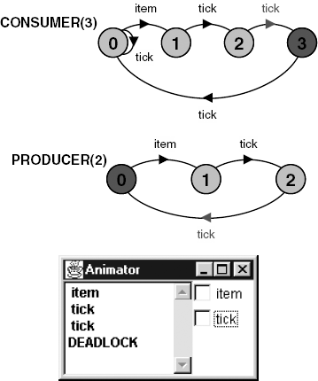
However, analysis of the system in which the producer is faster than the consumer detects the deadlock depicted in Figure 12.3.
||FASTER = (PRODUCER(2) || CONSUMER(3)).
The deadlock occurs because after the first item is produced and accepted by the consumer, the producer tries to produce another item after two clock ticks, while the consumer must accept a third clock tick before it can accept another item. The deadlock is caused by the timing inconsistency between producer and consumer. The producer is required to produce an item every two seconds while the consumer can only consume an item every three seconds. This kind of deadlock, caused by timing inconsistencies, is termed a time-stop. If we combine processes into a system and time-stop does not occur, we can say that the timing assumptions built into these processes are consistent.
Consider a system that connects the PRODUCER and CONSUMER processes of the previous section by a store for items as shown below:
STORE(N=3) = STORE[0],
     STORE[i:0..N] = (put -> STORE[i+1]
                  |when(i>0) get -> STORE[i-1]
                  ).

     ||SYS = ( PRODUCER(1)/{put/item}
             ||CONSUMER(1)/{get/item}
             ||STORE
             ).
We would reasonably expect that if we specify that items are consumed at the same rate that they are produced then the store would not overflow. In fact, if a safety analysis is performed then the following violation is reported:
Trace to property violation in STORE:
            put
            tick
            put
            tick
            put
            tick
            put
This violation occurs because the consumer has a choice between getting an item from the store, by engaging in the get action, and engaging in the tick action. If the consumer always chooses to let time pass, then the store fills up and overflows. To avoid this form of spurious violation in timed models, we must ensure that an action occurs as soon as all participants are ready to perform it. This is known as ensuring maximal progress of actions. We can incorporate maximal progress into our timed models by making the tick action low priority. For the example, a system that ensures maximal progress is described by:
||NEW_SYS = SYS>{tick}.Safety analysis of this system reveals no violations. Maximal progress means that after a tick, all actions that can occur will happen before the next tick. However, even though we assume that actions take a negligible amount of time, it would be unrealistic to allow an infinite number of actions to occur between ticks. We can easily check for this problem in a model using the following progress property, which asserts that a tick action must occur regularly in any infinite execution (see Chapter 7).
progress TIME = {tick}The following process violates the TIME progress property because it permits an infinite number of compute actions to occur between tick actions:
PROG = (start   -> LOOP | tick -> PROG),
     LOOP = (compute -> LOOP | tick -> LOOP).

     ||CHECK = PROG>{tick}.
The progress violation is reported by the analyzer as:
Progress violation: TIME
     Path to terminal set of states:
         start
     Actions in terminal set:
     {compute}
If we include an action that terminates the loop and then engages in a tick action, the progress property is not violated:
PROG = (start   -> LOOP | tick -> PROG),
     LOOP = (compute -> LOOP | tick -> LOOP
            |end -> tick -> PROG
            ).
This may seem strange since the loop still exists in the process. However, the end and compute actions are the same priority and consequently, with the fair choice assumption of Chapter 7, the compute action cannot be chosen an infinite number of times without the end action being chosen. The revised LOOP now models a finite number of iterations. The tick action following end means that the PROG process can only execute this finite LOOP once every clock tick. Consequently, the TIME progress property is not violated.
Incorporating time in models by the simple expedient of a global tick action is surprisingly powerful. In the following, we look at modeling techniques for situations that occur frequently in timed systems.
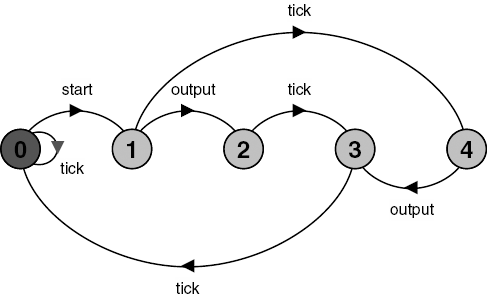
The examples we have seen so far produce an output or accept an input at a precise time, within the limitations of the discrete model of time. The INTERVAL process below produces an output at any time after Min ticks and before Max ticks. The LTS for the process is depicted in Figure 12.4.
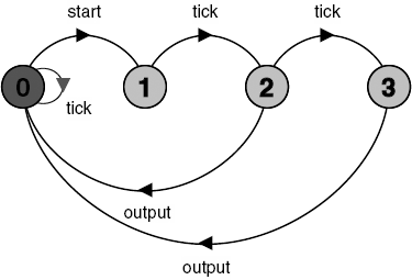
OUTPUT(Min=1,Max=3) =
       (start -> OUTPUT[1] | tick -> OUTPUT),
     OUTPUT[t:1..Max] =
       (when (t>Min && t<=Max) output ->OUTPUT
       |when (t<Max)           tick ->OUTPUT[t+1]
       ).
The technique of using choice with respect to the tick action allows us to model processes in which the completion time is variable, for example, due to loading or congestion.
A variation on the previous technique is a process that periodically produces an output at a predictable rate. However, the output may be produced at any time within the period. In communication systems, this kind of timing uncertainty is termed jitter. The JITTER process defined below is an example of how jitter can be modeled. Figure 12.5 depicts the LTS for the JITTER process.
JITTER(Max=2) =
       (start -> JITTER[1] | tick -> JITTER),
     JITTER[t:1..Max] =
       (output -> FINISH[t]
       |when (t<Max)   tick  -> JITTER[t+1]
       ),
FINISH[t:1..Max] =
(when (t<Max) tick -> FINISH[t+1]
|when (t==Max) tick -> JITTER
).Timeouts are frequently used to detect the loss of messages in communication systems or the failure of processes in distributed systems. Java provides a version of the wait() synchronization primitive that takes a timeout parameter – a wait() invocation returns either when notified or when the timeout period expires. The most elegant way to model a timeout mechanism is to use a separate process to manage the timeout, as shown below for a receive operation with a timeout. The timeout and receive processes are combined into a RECEIVER process.
TIMEOUT(D=1)
       = (setTO          -> TIMEOUT[0]
         |{tick,resetTO} -> TIMEOUT
         ),
     TIMEOUT[t:0..D]
       = (when (t<D) tick     -> TIMEOUT[t+1]
         |when (t==D)timeout  -> TIMEOUT
         |resetTO             -> TIMEOUT
         ).

     RECEIVE = (start   -> setTO -> WAIT),
     WAIT    = (timeout -> RECEIVE
               |receive -> resetTO -> RECEIVE
               ).

     ||RECEIVER(D=2) = (RECEIVE || TIMEOUT(D))
                     >{receive,timeout,start,tick}
                     @{receive,tick,timeout,start}.
In addition to tick, the start, receive and timeout actions are declared as low priority in the RECEIVER composite process. This is because maximal progress requires that an action take place when all the participants in that action are ready. However, the participants in interface actions depend on the system into which RECEIVER is placed, so we should not apply maximal progress to these actions within the RECEIVER process but later at the system level. Consequently, we give interface actions the same priority as the tick action. All internal actions have a higher priority. The minimized LTS for RECEIVER, which hides the internal actions concerned with setting and resetting the timeout, is depicted in Figure 12.6.

Timed concurrent systems can be implemented in Java by a set of threads which use sleep() and timed wait() to synchronize with time. We can characterize this as a thread-based approach since active entities in the model are translated into threads in an implementation. This approach to translating models into programs was used in the preceding chapters for non-timed systems. In this chapter, we exploit the time-driven nature of the models and use an event-based approach in which active entities are translated into objects that respond to timing events. Essentially, the tick action in the model becomes a set of events broadcast by a time manager to all the program entities that need to be aware of the passage of time. The organization of a timed system implementation conforms to the Announcer – Listener architecture described in Chapter 11, with the time manager acting as the announcer and timed objects as the listeners. We have chosen this event-based approach for two reasons. First, the translation from timed model to timed implementation is reasonably direct; and secondly, for timed systems with many activities the resulting implementation is more efficient than the thread-based approach since it avoids context-switching overheads. However, as discussed in the following, the approach also has some limitations when compared with a thread-based approach.
Each process in a timed model that has tick in its alphabet becomes a timed object in an implementation. A timed object is created from a class that implements the Timed interface listed in Program 12.1.
Each timed object is registered with the time manager, which implements a two-phase event broadcast. In phase 1, the pretick() method of each timed object is invoked and, in phase 2, the tick() method is invoked. The behavior of a timed object is provided by the implementation of these two methods. In the pre-tick phase, the object performs all output actions that are enabled in its current state. These may modify the state of other timed objects. In the tick phase, the object updates its state with respect to inputs and the passage of time. Two phases are needed to ensure that communication between timed objects completes within a single clock cycle. We clarify the translation from model processes into timed objects, with pretick() and tick() methods and the use of the TimeStop exception, in the examples that follow.
Example 12.1. Timed interface.
public interfaceTimed { void pretick()throwsTimeStop; void tick(); }
A version of the countdown timer model introduced in Chapter 2 is given below.
COUNTDOWN (N=3)   = COUNTDOWN[N],
     COUNTDOWN[i:0..N] =
       (when(i>0)  tick -> COUNTDOWN[i-1]
       |when(i==0) beep -> STOP
       ).
The COUNTDOWN process outputs a beep action after N ticks and then stops. The implementation is given in Program 12.2. The translation from the model is straightforward. Each invocation of the tick() method decrements the integer variable i. When i reaches zero, the next invocation of pretick() performs the beep action and the timer stops by removing itself from the time manager. The operation of TimeManager is described in the next section.
Example 12.2. TimedCountDown class.
classTimedCountDownimplementsTimed { int i; TimeManager clock; TimedCountDown(int N, TimeManager clock) { i = N;this.clock = clock; clock.addTimed(this);// register with time manager}publicvoid pretick() throws TimeStop {if(i==0) {// do beep actionclock.removeTimed(this);// unregister = STOP} }publicvoid tick(){ --i; } }
The next example implements the producer – consumer model of section 12.1.1. To keep the code succinct, the timed class definitions are nested inside the ProducerConsumer class of Program 12.3. The class creates the required instances of the Producer, Consumer and TimeManager classes.
Example 12.3. ProducerConsumer class.
classProducerConsumer { TimeManager clock =newTimeManager(1000); Producer producer =newProducer(2); Consumer consumer =newConsumer(2); ProducerConsumer() {clock.start();}classConsumerimplementsTimed {...}classProducerimplementsTimed {...} }
For convenience, the PRODUCER process is listed below:
PRODUCER(Tp=3) =
       (item -> DELAY[1]),
DELAY[t:1..Tp] =
(when(t==Tp) tick -> PRODUCER
|when(t<Tp) tick -> DELAY[t+1]
).Initially, the producer outputs an item and then waits for Tp clock ticks before outputting another item. The timed class that implements this behavior is listed in Program 12.4.
Example 12.4. Producer class.
classProducerimplementsTimed { int Tp,t; Producer(int Tp) {this. Tp = Tp; t = 1; clock.addTimed(this); }publicvoid pretick()throwsTimeStop {if(t==1) consumer.item(new Object()); }publicvoid tick() {if(t<Tp) { ++t;return; }if(t==Tp) { t = 1; } } }
An instance of the Producer class is created with t=1 and the consumer.item() method is invoked on the first pre-tick clock phase after creation. Each subsequent tick increments t until a state is reached when another item is output. The behavior corresponds directly with PRODUCER.
Now let us examine how the item() method is handled by the consumer. The timed model for the consumer is shown below. The consumer waits for an item and then delays Tc ticks before offering to accept another item.
CONSUMER(Tc=3) =
       (item -> DELAY[1] | tick -> CONSUMER),
DELAY[t:1..Tc] =(when(t==Tc) tick -> CONSUMER |when(t<Tc) tick -> DELAY[t+1] ).
The implementation of CONSUMER is listed in Program 12.5.
Example 12.5. Consumer class.
classConsumerimplementsTimed { int Tc,t; Object consuming = null; Consumer(int Tc) {this. Tc = Tc; t = 1; clock.addTimed(this); } void item(Object x)throwsTimeStop {if(consuming!=null)thrownew TimeStop(); consuming = x; }publicvoid pretick() {}publicvoid tick() {if(consuming==null)return;if(t<Tc) { ++t;return;}if(t==Tc) {consuming = null; t = 1;} } }
In the Consumer class, the tick() method returns immediately if the consuming field has the value null, implementing the behavior of waiting for an item. The item() method sets this field when invoked by the producer. When consuming is not null, the tick() method increments t until Tc is reached and then resets consuming to null indicating that the item has been consumed and that another item can be accepted. Effectively, consuming represents the DELAY states in the model. If the producer tries to set consuming when it is not null then a TimeStop exception is thrown. This signals a timing inconsistency in exactly the same way that a time-stop deadlock in the model is the result of a timing inconsistency. TimeStop is thrown if the producer tries to output an item when the previous item has not yet been consumed. As we see in the next section, a TimeStop exception stops the time manager and consequently, no further actions are executed. The implementation of producer – consumer has exactly the same property as the model. For correct execution, Tc must be less than or equal to Tp. Note that, in the Consumer class, the method pretick() has no implementation because the class has no outputs.
The operation of the two-phase clock cycle should now be clear. Methods on other objects are invoked during the pre-tick phase and the changes in state caused by these invocations are recognized in the tick phase. This ensures that actions complete in a single clock cycle. However, this scheme only approximates the maximal progress property of timed models. Maximal progress ensures that all actions that can occur happen before the next tick. Our implementation scheme only gives each timed object one opportunity to perform an action, when its pretick() method is executed. A multi-way interaction between timed objects thus requires multiple clock cycles. An example of a multi-way interaction would be a request action followed by a reply followed by an acknowledgment (threeway). Maximal progress in the model ensures that such a multi-way interaction would occur within a single clock cycle if no intervening tick events were specified. We could implement a multi-phase clock scheme to allow multi-way interaction in a single clock cycle, however this complexity might be better dealt with by reverting to a thread-based implementation scheme. In fact, the examples later in the chapter show that the two-phase scheme is sufficiently powerful to implement quite complex systems that exhibit the same behavior as their models. We take care that multi-way interaction within a single clock cycle is not required. This usually means that we introduce an intervening tick in the model, for example between a request and a reply.
In addition to the ease with which models can be translated into implementations, the event-based implementation scheme has the advantage, when compared to the thread-based scheme, that we do not have to synchronize access to shared objects. The activations of the tick() and pretick() methods of a timed object are indivisible with respect to other a ctivations of these methods. This is because the methods are dispatched sequentially by the time manager. Method dispatch incurs much less overhead than context switching between threads. Consequently, the event-based scheme is more efficient in systems with large numbers of time-driven concurrent activities. An example of such a system is presented in the final section of the chapter.
The TimeManager class (Program 12.6) maintains a list of all those timed objects which have registered with it using addTimed(). The pretick() and tick() methods are invoked on all Timed objects in this list by the TimeManager thread every delay milliseconds. The value of delay can be adjusted by an external control, such as a slider through the AdjustmentListener interface that the class implements.
The data structure used to hold the list of timed objects must be designed with some care. A pretick() or tick() method may cause a timed object to remove itself from the list. To ensure that such a removal does not destroy the integrity of the list data structure, we use an immutable list that does not change during an enumeration off it. If a removal occurs during a broadcast, this removal generates a new list which is used for the next broadcast. The class implementing the immutable list is given in Program 12.7.
Example 12.6. TimeManager class.
public classTimeManagerextendsThreadimplementsAdjustmentListener{volatileint delay;volatileImmutableList<Timed> clocked = null;publicTimeManager(int d) {delay = d;}publicvoid addTimed(Timed el) { clocked = ImmutableList.add(clocked,el); }publicvoid removeTimed(Timed el) { clocked = ImmutableList.remove(clocked,el); }publicvoid adjustmentValueChanged(AdjustmentEvent e) { delay = e.getValue(); }publicvoid run () {try{while(true) {try{for(Timed e: clocked) e.pretick();//pretick broadcastfor(Timed e:clocked) e.tick();//tick broadcast}catch(TimeStop s) {
System.out.println("*** TimeStop");
          return;
      }
      Thread.sleep(delay);
    }
  } catch (InterruptedException e){}
 }
}
Example 12.7. ImmutableList class.
public classImmutableList<T>implementsIterable<T> { ImmutableList<T> next; T item;privateImmutableList (ImmutableList<T> next, T item) { this.next = next; this.item=item; }public static<T> ImmutableList<T> add (ImmutableList<T> list, T item) {return newImmutableList<T>(list, item); }public static<T> ImmutableList<T> remove (ImmutableList<T> list, T target) {if(list == null) return null;returnlist.remove(target); }privateImmutableList<T> remove(T target) {if(item == target) {returnnext; }else{ ImmutableList<T> new_next = remove(next,target);if(new_next == next )returnthis;return newImmutableList<T>(new_next,item); } } }
The delay and clocked TimeManager fields (Program 12.6) are declared to be volatile since they can be changed by external threads. The keyword volatile ensures that the run() method reads the actual value of these fields before every broadcast. It prevents a compiler optimizing access by storing the fields in local variables or machine registers. If such an optimization occurred, the values would be read only once, when the run() method started, and it would not see subsequent updates.
The pretick() method allows a timed object to throw a TimeStop exception if it detects a timing inconsistency. This exception terminates the TimeManager thread. Consequently, a timing inconsistency in an implementation has the same behavior as a model with timing inconsistency – no further actions can be executed.
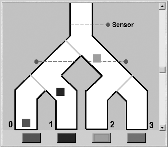
The parcel router problem is concerned with the simple parcel-sorting device depicted in Figure 12.7.
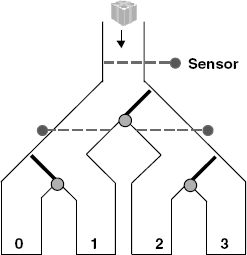
Parcels are dropped into the top of the router and fall by gravity through the chutes. Each parcel has a destination code that can be read by sensors. When a parcel passes a sensor, its code is read and the switch following the sensor is set to route the parcel to the correct destination bin. In this simple router, there are only four possible destinations numbered from zero to three. The switches can only be moved when there is no parcel in the way. The problem was originally formulated as a simple case study to show that specifications are not independent of implementation bias (Swartout and Balzer, 1982). It was called the Package Router problem. We have renamed packages to parcels to avoid possible confusion with Java packages.
In the following, we develop a timed model of the parcel router and then implement a simulation based on the model. We ignore gravity and friction and assume that parcels fall at a constant rate through chutes and switches.
The overall structure of the parcel router model is depicted in Figure 12.8. Parcels are fed into the routing network by a generator process and emerge from the network into one of four destination bins.
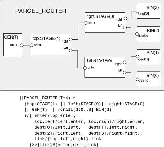
The generator process GEN, defined below, generates a parcel every T units of time. Each parcel contains the number of its destination. The generator picks a destination for a parcel using non-deterministic choice.
rangeDest = 0..3setParcel = {parcel[Dest]} GEN(T=3) = (enter[Parcel] -> DELAY[1] | tick -> GEN), DELAY[t:1..T] = (tick ->if(t<T)thenDELAY[t+1]elseGEN).
The destination bins are property processes that assert that the parcel delivered by the routing network to the bin must have the same destination number as the bin.
property
    BIN(D=0) = (dest[D].parcel[D] -> BIN)
+{dest[D][Parcel]}.We have subdivided the routing network into three stages. Each stage has an identical structure. The parameter to a stage determines its level in the routing network. The structure of the STAGE composite process is depicted in Figure 12.9.
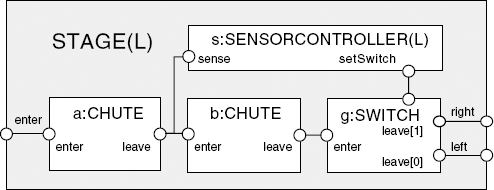
The composition expression which Figure 12.9 represents graphically is:
||STAGE(L=0) =
        ( a:CHUTE || b:CHUTE || g:SWITCH
        || s:SENSORCONTROLLER(L)
        )/{ enter/a.enter,   b.enter/{s.sense,a.leave},
g.enter/b.leave, s.setSwitch/g.setSwitch,
left/g.leave[0], right/g.leave[1],
tick/{a,b,g}.tick
} >{enter,left,right,tick}
@{enter,left,right,tick}.Each physical chute in the physical device is modeled by a set of CHUTE processes. A CHUTE process models the movement of a single parcel through a segment of a physical chute. To model a chute that can have n parcels dropping through it, we need n CHUTE processes. In modeling the system, we use two processes and so we are modeling a physical chute that can accommodate only two parcels. The CHUTE process is given below:
CHUTE(T=2) =
       (enter[p:Parcel] -> DROP[p][0]
       |tick            -> CHUTE
       ),
     DROP[p:Parcel][i:0..T] =
       (when (i<T)  tick     -> DROP[p][i+1]
       |when (i==T) leave[p] -> CHUTE
       ).
A parcel enters the chute and leaves after T units of time. We must be careful when composing CHUTE processes that the resulting composition has consistent timing. For example, the following system has a time-stop.
||CHUTES = (first:CHUTE(1) || second:CHUTE(2))
                /{second.enter/first.leave,
                  tick/{first,second}.tick}.
It happens when a parcel tries to enter the second CHUTE before the previous parcel has left. Time-stop in this context can be interpreted as detecting a parcel jam in the physical device. For consistent timing in a pipeline of CHUTE processes, each process must have a delay which is the same or greater than the delay of its successor.
This process detects a parcel by observing the action caused by a parcel passing from one CHUTE to the next. Based on the destination of the parcel, it computes how the switch should be set. This routing function depends on the level of the stage. Because the network is a binary tree, it is simply (destination > Level)&1 (in this expression context, > is the bit shift operator and & the bit-wise and operator). The function returns either zero, indicating left, or one, indicating right. SENSORCONTROLLER is not a timed process since we assume that detection of the parcel and computation of the route take negligible time. Each execution occurs within a clock cycle.
SENSORCONTROLLER(Level=0)
       = (sense.parcel[d:Dest] -> setSwitch[(d>Level)&1]
-> SENSORCONTROLLER).During the time that a parcel takes to pass through the parcel switch, it ignores commands from the SENSORCONTROLLER. This models the physical situation where a parcel is passing through the switch and consequently, the switch gate is obstructed from moving.
rangeDir = 0..1//Direction 0 = left, 1 = rightSWITCH(T=1) = SWITCH[0], SWITCH[s:Dir] = (setSwitch[x:Dir] -> SWITCH[x]//accept switch command|enter[p:Parcel] -> SWITCH[s][p][0] |tick -> SWITCH[s] ), SWITCH[s:Dir][p:Parcel][i:0..T] = (setSwitch[Dir] -> SWITCH[s][p][i]//ignore|when(i<T) tick -> SWITCH[s][p][i+1] |when(i==T)leave[s][p] -> SWITCH[s] ).
The SWITCH process extends the behavior of the CHUTE process with an additional component of its state to direct output and an extra action to set this state. SWITCH can be implemented by deriving its behavior, using inheritance, from the implementation of CHUTE.
Having completed the definition of all the elements of the PARCEL_ROUTER model, we are now in a position to investigate its properties. We first perform a safety analysis of a minimized PARCEL_ROUTER(3). This system feeds a new parcel every three timing units into the routing network. This produces the following property violation:
Trace to property violation in BIN(0):
enter.parcel.0
tick
tick
tick
enter.parcel.1
tick
tick
tick
enter.parcel.0
tick
tick
tick
enter.parcel.0
tick
dest.0.parcel.0
tick
tick
enter.parcel.0
tick
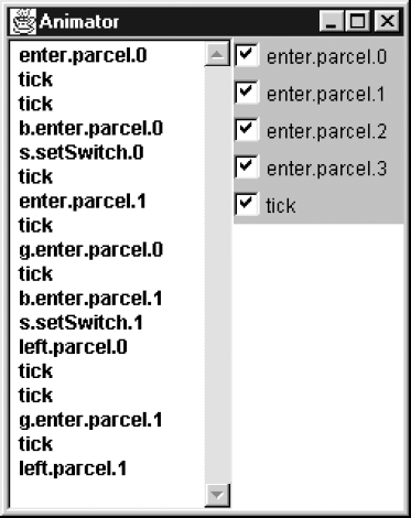
dest.0.parcel.1The trace clearly shows that a parcel intended for destination one has ended up in BIN zero. However, while it may be obvious to the reader why this has occurred, it is not clear from the trace since we have hidden the intermediate events that occur in each stage. We can elicit more information from the model in a number of ways. We can make internal actions visible and rerun the analysis or we can investigate the problem using the animator tool provided by LTSA. The second approach has the advantage that we do not need to modify the model in any way. We simply select STAGE as the target for analysis (with default level parameter as 0) and run the Animator using the following menu to specify the actions we wish to control.
menu TEST = {enter[Parcel],tick}The trace depicted in Figure 12.10 was produced by initially choosing an enter.parcel.0 action followed by three tick actions, then enter.parcel.1 followed by five ticks. This is the trace produced by the safety violation, without the subsequent parcel entries. The Animator trace clearly exposes the reason for the violation. The first parcel is still in the switch when the sensor detects the second parcel and tries to set the switch to direction 1. Since the first parcel is in the switch, the s.setSwitch.1 action is ignored and the switch does not change. Consequently, the second parcel follows the first in going to the left when it should have been switched to the right.
The physical interpretation of the problem is that parcels are too close together to permit correct routing. We can check this intuition by analyzing a system with a slower parcel arrival rate, PARCEL_ROUTER(4). Safety analysis finds no problems with this system and progress analysis demonstrates that the TIME property is satisfied.
In the next section, we describe a simulation of the parcel router based on the model. This implementation faithfully follows the model in allowing parcels that are too close together to be misrouted.
The display for the parcel router simulation is shown in Figure 12.11. A new parcel for a particular destination is generated by pressing the button beneath that destination. Parcels that arrive at the wrong destination flash until they are replaced by a correct arrival. The speed of the simulation can be adjusted using the slider control to the right of the display. This controls the TimeManager described in section 12.2.2.
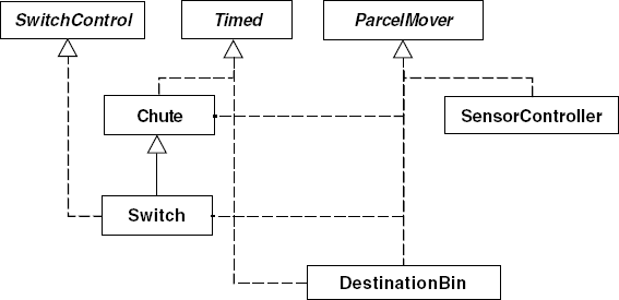
In describing the parcel router implementation, we concentrate on the interfaces and classes shown in Figure 12.12. These classes implement the timed behavior of the simulation. Display is implemented by the ParcelCanvas and Parcel classes. Each Parcel object is registered with the ParcelCanvas, which displays the parcel at its current position once per clock cycle. In addition, the ParcelCanvas displays the background and the current state of each switch. The Parcel and ParcelCanvas code can be found on the website that accompanies this book.
To permit flexible interconnection of Chute, Switch, SensorController and DestinationBin objects, each class implements the ParcelMover and SwitchControl interfaces listed in Program 12.8. The latter interface is required to allow switches to be connected to controllers.
The Chute class listed in Program 12.9 is a direct translation of the CHUTE process defined in the previous section using the method described in section 12.2.1. If the current field is not null then the chute contains a parcel. After T clock cycles this parcel is transferred to the ParcelMover object referenced by the next field. This field is initialized when the configuration of chutes, switches, etc. is constructed by the ParcelRouter applet.
Example 12.8. ParcelMover and SwitchControl interfaces.
interfaceParcelMover { void enter(Parcel p)throwsTimeStop; }interfaceSwitchControl { void setSwitch(int direction); }
The Switch class listed in Program 12.10 is derived from Chute. A Switch object has references to the ParcelMover objects to its left and right. The setSwitch method sets the next field of the super class to one of these if there is no parcel currently occupying the switch. If there is, the command to switch is ignored, as in the model. Setting the next field means that when a parcel leaves, it is sent to the ParcelMover referenced by either left or right.
The SensorController class is listed in Program 12.11. Parcels pass through within a single clock cycle. The class is not aware of time and does not implement the Timed interface. Only model processes that have tick in their alphabets need to be implemented as Timed classes.
The ParcelRouter applet class contains a set of methods that create and "wire together" the parts of the simulation. The method listed below creates an assembly that corresponds to the STAGE composite process of the model.
Example 12.9. Chute class.
classChuteimplementsParcelMover, Timed {protectedint i,T,direction;protectedParcel current = null; ParcelMover next = null; Chute(int len, int dir) { T = len; direction = dir;}// parcel enters chutepublicvoid enter(Parcel p)throwsTimeStop {if(current!=null)throw newTimeStop(); current = p; i = 0; }publicvoid pretick()throwsTimeStop {if(current==null)return;if(i == T) { next.enter(current); //package leaves chutecurrent = null; } }publicvoid tick(){if(current==null)return;//update display position of parcel++i; current.move(direction); } }
Example 12.10. Switch class.
classSwitchextendsChuteimplementsSwitchControl { ParcelMover left = null; ParcelMover right = null;privateParcelCanvas display;privateint gate; Switch(int len, int dir, int g, ParcelCanvas d ) {super(len,dir); display = d; gate = g;}
publicvoid setSwitch(int direction) {if(current==null) {// nothing passing through switchdisplay.setGate(gate,direction);if(direction==0) next = left;elsenext = right; } } }
Example 12.11. SensorController class.
classSensorControllerimplementsParcelMover { ParcelMover next; SwitchControl controlled;protectedint level; SensorController(int level){this.level=level;}// parcel enters and leaves within one clock cyclepublicvoid enter(Parcel p) throws TimeStop { route(p.destination); next.enter(p); }protectedvoid route(int destination) { int dir = (destination>level) & 1; controlled.setSwitch(dir); } }
ParcelMover makeStage
         (ParcelMover left, ParcelMover right,
          int fallDir, // movement direction for parcel display
          int level,   // 0 or 1 as in the model
          int gate     // identity of gate for display purposes
         )
{
// create parts and register each with TimeManager ticker
Chute a = new Chute(16,fallDir);
ticker.addTimed(a);
SensorController s = new SensorController(level);
Chute b = new Chute(15,fallDir);
ticker.addTimed(b);
Switch g = new Switch(12,fallDir,gate,display);
ticker.addTimed(g);
// wire parts together
a.next = s; s.next = b; s.controlled = g;
b.next = g; g.left = left; g.right = right;
return a;
}The method exhibits a pleasing correspondence with the STAGE model. The model process prefix names become object references and the model relabels become reference assignments.
The DestinationBin class, which may be found on the website that accompanies this book, accepts a Parcel object and displays it in a fixed position. When a new parcel arrives, the old parcel is removed from the display. Parcels that arrive at the wrong destination are flashed by hiding and revealing them on alternate clock cycles.
The reader is encouraged to run the PackageRouter applet and observe that its behavior is as predicted by the model. The restriction that only one-way interactions can be supported by the clocking scheme has not caused a problem in this example. Even though the interaction between Chute, SensorController and Switch requires more than one method call in a clock cycle, it is still a uni-directional interaction in which a chute output causes an input to another chute and a switch.
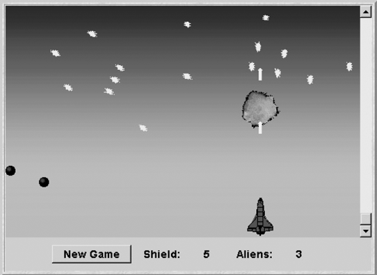
The final example of a timed system is a simple video arcade game. The display is depicted in Figure 12.13. The spaceship can be moved around the screen using the cursor keys. Pressing the space bar on the keyboard launches a missile from the spaceship. Missiles move up the display and appear as white arrows on the display. Aliens, depicted as spheres, drop from the top of the screen and explode when hit by a missile. When an alien collides with the spaceship, an explosion occurs and the shield strength of the spaceship is reduced. The game terminates when the shield strength drops to zero. The objective, as is usual in this style of game, is to shoot as many aliens as possible.
Video games involve many active entities, called sprites, which move around independently and concurrently. A sprite has a screen representation and a behavior. Sprites may interact when they collide. In Space Invaders, the sprites are the spaceship, aliens, missiles and explosions. Sprites are essentially concurrent activities, which we could consider implementing as threads. However, this would result in a game with poor performance due to the synchronization and context-switching overheads involved. A much better scheme is to implement sprites as timed objects. Each sprite has an opportunity to move once per clock cycle. This has the advantage that it is simple to synchronize screen updates with sprite activity. We simply repaint the screen once per clock cycle.
Sprites move about in the two-dimensional space depicted in Figure 12.14. In an implementation, the coordinates refer to screen locations. In the model, we use a smaller space to permit analysis.
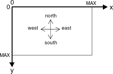
The coordinate system is represented in the model by the following definitions. In the interests of simplicity, the width of the game space is assumed to be the same as its depth. The undef label is used to specify the coordinate of a sprite that has not been created and consequently does not have a defined position on the screen.
constMAX = 4rangeD = 0..MAXsetCoord = {[D][D],undef} //(x,y)
The entities that comprise the Space Invaders game have behavior in common with respect to the way that they move about in the game space. We model this common behavior as the SPRITE process listed below. The behavior of the spaceship, missiles and aliens is defined using this process.
SPRITE =
       (create[x:D][y:D] -> SPRITE[x][y]
       |tick -> SPRITE
       |pos.undef -> SPRITE
       ),
     SPRITE[x:D][y:D] =
       (pos[x][y] -> SPRITE[x][y]
       |tick ->
        (north -> if y>0   then SPRITE[x][y-1] else END
        |south -> if y<MAX then SPRITE[x][y+1] else END
        |west  -> if x>0   then SPRITE[x-1][y] else END
        |east  -> if x<MAX then SPRITE[x+1][y] else END
| {rest,action[x][y]} -> SPRITE[x][y]
)
),
END = (end -> SPRITE).Before a sprite is created, its location is undefined. A query using the action pos will return the undef value for its location. After the create action, pos returns a valid coordinate for the sprite's current location. At each clock tick, a sprite can move in one of four directions, or it can remain in the same position (rest action). The sprite implementation described in the next section allows a sprite to move in one of eight directions; however, four directions are sufficient detail for modeling purposes. In addition to moving, a sprite can instigate an action during a clock cycle. When a sprite moves out of the game space, it indicates that it has terminated by performing the end action. In an implementation, a sprite would then be garbage collected. In the model, the sprite goes back to the state in which it can be created. As described in Chapter 9, we use cyclic behavior to model dynamic creation. The set of actions that the SPRITE process can engage in – excluding tick and the position query pos –is specifiedby:
set Sprite =
{north,south,west,east,rest,action[D][D],create[D][D]}An alien is a sprite that moves down the screen. Consequently, we can specify its behavior by constraining the movement of the SPRITE process. In the model, an alien starts at the top of the screen and moves vertically down; in the implementation, it can also move diagonally down.
ALIEN_CONSTRAINT =
       (create[D][0] -> MOVE),
     MOVE =
       (south -> MOVE | end -> ALIEN_CONSTRAINT)
       +Sprite.

     ||ALIEN = (SPRITE || ALIEN_CONSTRAINT).
The constraint permits an alien to be created at any x-position at the top of the screen and only permits it to move south and then end when it leaves the screen. The ALIEN composite process permits only these actions to occur since the constraint has the Sprite alphabet.
The behavior of the missile sprite is defined in exactly the same way. In this case, the missile is only permitted to move north, up the screen.
MISSILE_CONSTRAINT =
        (create[D][MAX] -> MOVE),
     MOVE =
       (north -> MOVE | end -> MISSILE_CONSTRAINT)
       + Sprite.

||MISSILE = (SPRITE || MISSILE_CONSTRAINT).The spaceship has more complex behavior. It is constrained to moving horizontally at the bottom of the screen, either east or west, or staying in the same position, rest. It is created in the center of the screen and is constrained not to move off the screen. The spaceship can perform an action, which is used to create a missile, as explained later. In fact, the implementation permits the spaceship to move up and down the screen as well. However, horizontal movement is sufficient detail for us to gain an understanding of the operation of the system from the model.
SPACESHIP_CONSTRAINT =
        (create[MAX/2][MAX] -> MOVE[MAX/2]),
     MOVE[x:D] =
        ( when (x>0)  west -> MOVE[x-1]
        | when (x<MAX) east -> MOVE[x+1]
        | rest -> MOVE[x]
        | action[x][MAX] -> MOVE[x]
        ) + Sprite.

     ||SPACESHIP =(SPRITE || SPACESHIP_CONSTRAINT).
Collision detection is modeled by the COLLIDE process which, after a tick, queries the positions of two sprites and signals a collision through the action explode if their positions coincide. Undefined positions are excluded. In the implementation, the detection of a collision results in the creation of an explosion sprite that displays a series of images to create the appropriate graphic appearance. In the model, we omit this detail.
COLLIDE(A='a, B='b) =
       (tick -> [A].pos[p1:Coord] -> [B].pos[p2:Coord]
        -> if (p1==p2 && p1!='undef && p2!='undef) then
              ([A][B].explode -> COLLIDE)
           else
              COLLIDE
).The composite process SPACE_INVADERS models a game that, in addition to the spaceship, permits only a single alien and a single missile to appear on the screen. This simplification is required for a model of manageable size. However, we have defined sprites as having cyclic behavior that models recreation. Consequently, the alien can reappear in different start positions and the spaceship can launch another missile as soon as the previous one has left the screen. The model captures all possible behaviors of the combination of spaceship, alien and missile.
To model launching a missile, we have associated the spaceship's action with the missile's create by relabeling. Two collision detectors are included to detect spaceship–alien and alien–missile collisions.
||SPACE_INVADERS =
        ( alien   :ALIEN
        || spaceship:SPACESHIP
        || missile:MISSILE
        || COLLIDE('alien,'spaceship)
        || COLLIDE('missile,'alien))
        /{spaceship.action/missile.create,
          tick/{alien,spaceship,missile}.tick}
>{tick}.Safety analysis of SPACE_INVADERS does not detect a time-stop and progress analysis demonstrates that the TIME progress property is satisfied. Further, the progress properties:
progressSHOOT_ALIEN={missile.alien.explode}progressALIEN_SHIP ={alien.spaceship.explode}
are satisfied, showing that both alien – missile and alien – spaceship collisions can occur. To gain an understanding of the operation of the model, we can animate it to produce example execution traces. An alternative approach to producing sample traces is to use safety properties as follows. Suppose we wish to find a trace that results in a collision between an alien and a missile. We specify a safety property that the action missile.alien.explode should not occur and analyze the system with respect to this property:
property ALIEN_HIT = STOP + {missile.alien.explode}.
||FIND_ALIEN_HIT = (SPACE_INVADERS || ALIEN_HIT).
The trace produced is:
Trace to property violation in ALIEN_HIT:
          alien.create.1.0
          spaceship.create.2.4
          tick
          alien.south
          spaceship.west
          missile.pos.undef
          alien.pos.1.1
          spaceship.pos.1.4
          tick
          alien.south
          spaceship.action.1.4 – missile launched
          missile.pos.1.4
          alien.pos.1.2
          spaceship.pos.1.4
          tick
          alien.south
          missile.north
          missile.pos.1.3
          alien.pos.1.3
          missile.alien.explode
Exactly the same approach can be used to find a trace leading to a spaceship – alien collision.
The emphasis of the Space Invaders model is not so much on demonstrating that it satisfies specific safety and liveness properties but rather as a means of investigating interactions and architecture. After all, the program is far from a safety-critical application. However, in abstracting from implementation details concerned with the display and concentrating on interaction, the model provides a clear explanation of how the program should operate. In addition, it provides some indication of how the implementation should be structured. For example, it indicates that a CollisionDetector class is needed and confirms that a Sprite class can be used to implement the common behavior of missiles, aliens and the spaceship.
The implementation of the Space Invaders program is large in comparison to the example programs presented previously. Consequently, we restrict ourselves to describing the structure of the program using class diagrams. The translation from timed processes to timed objects should be clear from examples presented in earlier sections of this chapter. The reader can find the Java code for each of the classes we mention on the website that accompanies this book.
The display for the Space Invaders program is handled by the two classes depicted in Figure 12.15. A Sprite is created with an initial position and an image. The SpriteCanvas maintains a list of sprites. Every clock tick, the SpriteCanvas calls the paint() method of each sprite on its list. The sprite then draws its image at its current position.
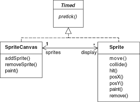
The move() method has a direction parameter that specifies one of eight directions in which the sprite can move. It is called by a subclass each clock cycle to change the position of the sprite. The collide() method tests whether the sprite's bounding rectangle intersects with the sprite passed as a parameter. The hit() method is called by the collision detector when a collision is detected. PosX() and PosY() return the current x and y coordinates of the sprite.
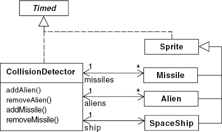
The collision detector maintains a list of the alien sprites and missile sprites and a reference to the spaceship sprite as shown in Figure 12.16. Every clock cycle, the detector determines whether each alien has collided with either a missile or the spaceship. If a collision is detected, the hit() methods of the sprites involved in the collision are invoked.
The method listed below is the implementation provided for the hit() method in the Alien class.
publicvoid hit() {newExplosion(this); SpaceInvaders.score.alienHit(); SpaceInvaders.detector.removeAlien(this); remove();// remove from SpriteCanvas}
The method creates a new explosion sprite at the same location as the alien, records an alien hit on the scoreboard and removes the alien from the collision detector and the display. The CollisionDetector, Alien, Missile and Spaceship classes implement the essential behavior of the game. These classes correspond to the COLLIDE, ALIEN, MISSILE and SPACESHIP model processes.
The SpaceInvaders applet class creates the spaceship, the alien generator, the missile launcher and the score board in addition to the display, time manager and collision detector as shown in Figure 12.17.
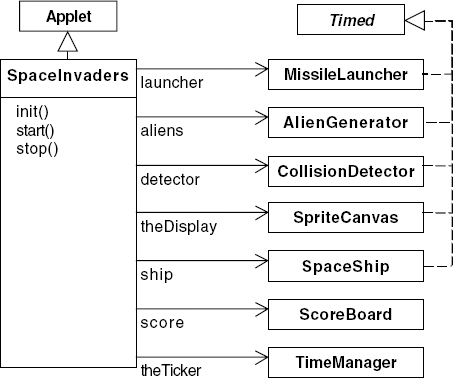
The AlienGenerator waits for a random number of clock cycles and then creates a new alien with a randomly chosen start position and a random downward direction. The MissileLauncher creates a new missile when the space bar is pressed. The x-coordinate of the new missile is the current position of the spaceship. The classes included in Figure 12.17 provide the infrastructure for scoring and the creation and display of sprites.
The collision detector and display run during the pre-tick clock phase; the remaining program actions, such as sprite movement, occur during the tick phase. This permits the display to render a consistent set of positions and for the effect of hits to be computed during tick processing. However, in reality, we could implement this sort of program using only a single-phase clock. This is because the clock ticks rapidly and, since the screen is updated every cycle, any inconsistencies which resulted from an action happening over two clock cycles rather than one would not be visible to a user.
This chapter has presented a discrete approach to modeling and implementing timed systems. The passage of time is signaled by regular successive ticks of a clock. In models, this tick appears as an action that is shared by the processes for which behavior depends on the passage of time. In implementations, the tick is an event broadcast by a time manager.
In discrete time models, we saw that the composition of processes with inconsistent timing resulted in a deadlock. This sort of deadlock is termed a time-stop. The order in which actions can occur in a timed model is restricted by making a maximal progress assumption. This ensures that an action occurs as soon as all participants are ready to perform it. Maximal progress is true for a model when we make the tick action low priority. This ensures that all ready actions occur within a clock cycle. Maximal progress thus reflects the implementation assumption that actions take negligible time to execute.
We described an implementation approach for timed systems that is event-based rather than thread-based. In this approach, each model process that has tick in its alphabet is translated into a timed object. Timed objects are invoked regularly by a time manager that dispatches timing events. We use a two-phase scheme that requires a pre-tick and tick event dispatch. Timed objects produce outputs during the pre-tick phase and compute the next state based on received inputs during the tick phase. This scheme permits one-way communication interactions to occur atomically within a single clock cycle. It was pointed out that multi-way interactions within a single clock cycle are not supported by this scheme. However, this did not cause problems in the example programs. The advantage of using timed objects rather than threads to implement timed processes is concerned with runtime efficiency. Timed objects are activated by method invocation, which has a lower overhead than context-switching threads. Further, since the pre-tick and tick methods run sequentially, there is no synchronization overhead to ensure mutual exclusion. Lastly, for programs largely concerned with display, the approach naturally synchronizes screen updates from multiple activities.
We should also point out some of the disadvantages of the event-based approach or the reader might wonder why we have devoted the main part of the book to a thread-based approach. Threads abstract from the detail of how activities should be scheduled to organize interaction. We saw that the timed approach was limited to uni-directional interactions in a single clock cycle. More complex interaction needs to be explicitly scheduled with either a multi-phase clock or, alternatively, over multiple clock cycles. This rapidly becomes unmanageable for complex interactions. Further, the event-based scheme required a timed object to examine its state every clock cycle to determine whether an event has occurred. A thread-based implementation may incur lower overhead for systems in which activities do not perform some action every clock cycle. The thread scheduler dispatches a thread only when there is some work for it to do.
Finally, we note that the model-based approach to concurrent programming permits a designer the flexibility to use either an event-based or thread-based implementation scheme or indeed a hybrid. We use the same modeling and analysis techniques for both implementation approaches.
A comprehensive treatment of using discrete time in the context of CSP may be found in Roscoe's book (1998). We have adapted the approach presented there to fit with the modeling tools and techniques used in this book. However, our approach is essentially the same and much credit is due to Roscoe for providing the first generally accessible introduction to this style of modeling time.
It was explicitly stated in the introduction that the timed systems we deal with arenotreal-timeinthesenseofguaranteeing deadlines. The interested reader will find that there is a vast literature on the specification, verification and analysis of real-time systems. A good starting point is a book edited by Mathai Joseph which presents a number of techniques with respect to the same case study (1996). One of the techniques presented is Timed CSP, which uses a dense continuous model of time in contrast to the discrete model we present. Continuous time is more expressive but leads to difficulties in automated analysis.
12.1 Define a process that models a timed single-slot buffer. The buffer should both wait to accept input and wait to produce output. The buffer requires a minimum of T time units to transfer an item from its input to its output.
12.2 Using the process defined in exercise 12.1, define a two-slot timed buffer and explore its properties. Determine the timing consistency relationship between the delays for the two buffers. Explore the effect of applying maximal progress by making
ticklow priority.12.3 Implement the timed buffer process of exercise 12.1 as a timed object and explore the runtime behavior of a system composed of these objects with producer and consumer timed objects. (Note: Waiting to produce an output is implemented in timed systems by balking rather than throwing a time-stop. By balking, we mean that the method performing the output returns a boolean indicating whether or not the output was possible. If it fails, it is retried on the next clock cycle.)
12.4 An electric window in a car is controlled by two press-button switches: up and down. When the up button is pressed, then the window starts closing. If the up button is pressed for less than T seconds then the window closes completely. If the up button is pressed for more than T seconds then when the button is released, the window stops closing. The down button works in exactly the same way, except that the window opens rather than closes. A mechanical interlock prevents both buttons being pressed at the same time.
The window is moved by a motor that responds to the commands start_close, stop_close, start_open and stop_open. Two sensor switches, closed and opened, detect, respectively, when the window is fully closed and when it is fully open. The window takes R units of time to move from the completely open position to the completely closed position or vice versa.
Define a timed model for the electric window system in FSP. Specify safety properties that assert that the motor is not active when the window is fully closed or fully opened.
12.5 Translate the model of the electric window system into a Java implementation using timed objects.