
In Chapter 7, we saw that a property is an attribute of a program that is true for every possible execution of that program. We used property processes to specify safety properties and progress properties to express a limited but very common form of liveness property. Here we introduce logical descriptions of properties that capture both safety and liveness.
What do we mean by a logical description? We mean an expression composed out of propositions by logical operators such as and, or, not. A proposition is a statement that is either true or false. It can of course be formed from more primitive propositions by the logical operators and so the overall logical description is itself a proposition. Java already uses this form of expression in the assert construct. For example, using this construct we can assert that after executing some statements it should be true that variable i has the value 0 and variable j has the value 1: (assert i==0 && j==1).
The Java assert construct lets us specify a proposition concerning the state of selected variables that should be true at a particular point in the execution of a program. Of course, if this point is in a loop, it will be visited repeatedly. In our models, we wish to specify propositions that are true for every possible execution of a program without explicit reference to a particular point in the execution of that program. Furthermore, we wish to specify properties independently from models. A logic that permits us to do this is linear temporal logic. A proposition in this logic describes a set of infinite sequences for which the proposition is true. A program execution is essentially a sequence of states and so a program satisfies a linear temporal logic proposition if all its executions belong to the set described by the formula.
How can we refer to states when our LTS models are essentially based on actions or events? This chapter introducesfluentsasameansofdescribingabstract states of our models. We show how logical properties for both safety and liveness can be specified in terms of fluents and analyzed using LTSA.
The primitive propositions used to construct assertions in Java are concerned with the values of variables, for example, i==0. They are propositions concerning the state of a program as represented by the values of the program's variables. However, our models are focused on interaction and as such they describe sequences of actions and do not explicitly describe state. What should be the primitive propositions that we use in the logical description of properties? One possibility would be to make the occurrence of an action a proposition such that for an action a, the synonymous proposition a would be true when the action occurred and false at every other time. The problem here is that, as we saw in Chapter 3, we model concurrent execution as an interleaved sequence of actions which we call a trace. Consequently it would always be the case that only one action proposition could be true at any one instant. This makes it difficult to describe quite simple properties. As a result, we have taken an approach which allows us to map an action trace into a sequence of abstract states described by fluents.
Note
fluent FL = <{s1,...sn},{e1..en}> initially B defines a fluent FL that is initially true if the expression B is true and initially false if the expression B is false. FL becomes true when any of the initiating actions {s1,...sn} occur and false when any of the terminating actions {e1..en} occur. If the term initially B is omitted then FL is initially false. The same action may not be used as both an initiating and terminating action.
In other words, a fluent holds at a time instant if and only if it holds initially or some initiating action has occurred, and, in both cases, no terminating action has yet occurred. The following fragment defines a fluent LIGHT which becomes true when the action on occurs and false when the action off or power_cut occurs.
constFalse = 0constTrue = 1fluentLIGHT = <{on}, {off, power_cut}>initiallyFalse
We can think of the above fluent as capturing the state of a light such that when the light is on, the fluent LIGHT is true and when the light is off, the fluent LIGHT is false. We can define indexed families of fluents in the same way that we define indexed families of processes:
fluent LIGHT[i:1..2] = <{on[i]}, {off[i], power_cut}>This is equivalent to defining two fluents:
fluentLIGHT_1 = <{on[1]}, {off[1], power_cut}>fluentLIGHT_2 = <{on[2]}, {off[2], power_cut}<
Fluents are defined by a set of initiating actions and a set of terminating actions. Consequently, given the alphabet α of a system, we can define a fluent for each action a in that alphabet such that the initiating set of actions for the fluent a is {a} and the terminating set of actions is α∪{τ}−{a}. In other words, the fluent for an action becomes true immediately that action occurs and false immediately the next action occurs. The next action may be the silent action τ. We can also use a set of actions in a fluent expression. The logical value of this is the disjunction (or) of each of the actions in the set. We can freely mix action fluents and explicitly defined fluents in fluent expressions. An example is given in the next section.
We can combine fluents with the normal logical operators. If we wished to characterize the state in which two lights are on, this would be the expression LIGHT[1] && LIGHT[2]. The state in which either light is on would be LIGHT[1] || LIGHT[2]. This latter would also be true if both lights were on. Fluent expressions can be formed using the following logical operators:
&& | conjunction (and) |
|| | disjunction (or) |
| negation (not) |
| implication |
| equivalence |
For example, given the fluents:
fluentPOWER = <power_on, power_off>fluentLIGHT = <on, off>
the expression LIGHT->POWER states our expectation that, for the light to be on, the power must also be on. We do not expect that if the power is on the light need necessarily be on as well.
If we wish to express the proposition that all lights are on, we can use the expression:
forall[i:1..2] LIGHT[i]This is exactly the same as LIGHT[1] && LIGHT[2]. In a similar way, if we wish to express the proposition that at least one light is on, we can state:
exists[i:1..2] LIGHT[i]This is exactly the same as LIGHT[1] || LIGHT[2].
An expression that combines an action fluent and an explicitly defined fluent is (getkey && LIGHT[1]) which is true when the getkey action occurs when the LIGHT fluent is true – i.e., the light has previously been turned on.
Fluents let us express properties about the abstract state of a system at a particular point in time. This state depends on the trace of actions that have occurred up to that point in time. To express propositions with respect to an execution of a model, we need to introduce some temporal operators.
To illustrate the expression of safety properties using fluents, we return to the mutual exclusion example of section 7.1.2.
const N = 2

LOOP = (mutex.down -> enter -> exit -> mutex.up -> LOOP).

||SEMADEMO = (p[1..N]:LOOP
          || {p[1..N]}::mutex:SEMAPHORE(1)).
The abstract states of interest here are when each LOOP process enters its critical section. We express these states with fluents:
fluent CRITICAL[i:1..N] = <p[i].enter, p[i].exit>We can express the situation in which two processes are in their critical sections at thesametimeas CRITICAL[1] && CRITICAL[2]. This situation must be avoided at all costs since it violates mutual exclusion. How do we assert that this situation does not occur at any point in the execution of the SEMADEMO system?
Note
The linear temporal logic formula []F – always F – is true if and only if the formula F is true at the current instant and at all instants in the future.
Given this operator, we can now express the property that at all times in any execution of the system, CRITICAL[1] && CRITICAL[2] must not occur. This is:
assert MUTEX = []!(CRITICAL[1] && CRITICAL[2])This property is checked by compiling it into a safety property process. As described in Chapter 7, the check is then performed by composing this property with the system and performing an exhaustive search for the ERROR state. The property process compiled from MUTEX above is depicted in Figure 14.1.
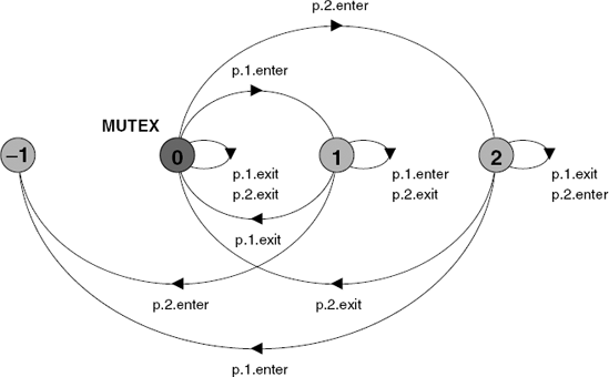
The MUTEX property is not violated with the semaphore initialized to one; however if we initialize the semaphore to two (i.e. SEMAPHORE(2)) then a check of the MUTEX property against the SEMADEMO system produces the following trace:
Trace to property violation in MUTEX:
           p.1.mutex.down
           p.1.enter           CRITICAL.1
           p.2.mutex.down      CRITICAL.1
           p.2.enter           CRITICAL.1 && CRITICAL.2
The LTSA annotates the trace with the names of the fluents that are true when the action on the left occurs. So, when the action p.2.enter occurs, both of the CRITICAL fluents are true, violating mutual exclusion. The general expression of the mutual exclusion property for N processes is:
assertMUTEX_N = []!(exists[i:1..N-1] (CRITICAL[i] && CRITICAL[i+1..N]))
This asserts that it is always the case that no pair of processes exist with CRITICAL true. CRITICAL[i+1..N] is a short form for the disjunction exists [j:i+1..N] CRITICAL[j].
The single-lane bridge problem was described in section 7.2. The required safety property was that it should never be the case that a red car (moving from left to right) should be on the bridge at the same time as a blue car (moving from right to left). The following fluents capture the states of red cars and blue cars being on the bridge.
constN = 3// number of each type of carrangeID= 1..N// car identitiesfluentRED[i:ID] = <red[i].enter, red[i].exit>fluentBLUE[i:ID] = <blue[i].enter, blue[i].exit>
The situation in which one or more red cars are on the bridge is described by the fluent expression exists [i:ID] RED[i] and similarly for blue cars exists [j:ID] BLUE[j]. The required ONEWAY property asserts that these two propositions should never hold at the same time.
assertONEWAY = []!(exists[i:ID] RED[i] &&exists[j:ID] BLUE[j])
When checked in the context described in section 7.2.1 with no BRIDGE process to constrain car behavior, the following safety violation is produced:
Trace to property violation in ONEWAY:
           red.1.enter         RED.1
           blue.1.enter        RED.1 && BLUE.1
Since propositions of the form exists [i:R] FL[i] can be expressed succinctly as FL[R], we can rewrite ONEWAY above as:
assert ONEWAY = []!(RED[ID] && BLUE[ID])This is a considerably more concise description of the required property than that achieved using property processes in section 7.2.1. In addition, it expresses the required property more directly. This is usually the case where a safety property can be expressed as a relationship between abstract states of the system described as fluents. Unsurprisingly where the required property is concerned with the permitted order of actions, direct specification using property processes is usually best.
Finally, safety properties of the form [] P as we have described here are by far the commonest form of safety properties expressed in temporal logic; however, there are many other forms of safety properties which use additional temporal operators. These operators are described later.
A safety property asserts that nothing bad ever happens whereas a liveness property asserts that something good eventually happens. Linear temporal logic provides the eventually operator which allows us to directly express the progress properties we introduced in Chapter 7.
Note
The linear temporal logic formula <> F – eventually F – is true if and only if the formula F is true at the current instant or at some instant in the future.
We can now assert for the single-lane bridge example that eventually the first red car must enter the bridge:
assert FIRSTRED = <>red[1].enter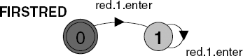
This is compiled into the transition system shown in Figure 14.2. This is a special form of transition system known as a Büchi automaton after its originator. A Büchi automaton recognizes an infinite trace if that trace passes through an acceptance state infinitely often. The example of Figure 14.2 has a single acceptance state marked by two concentric rings. It should be clear that any trace containing the action red[1].enter is not accepted by this automaton since the action will move the automaton irretrievably out of the initial acceptance state.
In fact, the Büchi automaton of Figure 14.2 accepts the set of infinite traces represented by the negation of the FIRSTRED property – that is, !<>red[1].enter. To check whether an assertion holds, the LTSA constructs a Büchi automaton for the negation of the assertion and then checks whether there are any infinite traces that are accepted when the automaton is combined with the model. This check can be performed efficiently since it is a search for acceptance states in strongly connected components. If none are found then there is no trace that satisfies the negation of the property and consequently the property holds. We discussed strongly connected components and their relationship to infinite executions in Chapter 7. In checking liveness properties, we make exactly the same fair choice assumption as was made in Chapter 7. The property is satisfied for the basic bridge model but not for the congested model defined by:
||CongestedBridge
           = SingleLaneBridge > {red[ID].exit,blue[ID].exit}.
The following property violation is reported for a system with two red cars and two blue cars:
Violation of LTL property: @FIRSTRED
     Trace to terminal set of states:
           blue.1.enter
     Cycle in terminal set:
           blue.2.enter
           blue.1.exit
           blue.1.enter
           blue.2.exit
     LTL Property Check in: 10ms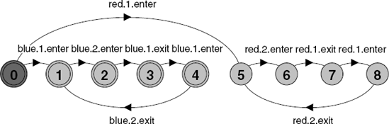
The model, combined with the FIRSTRED property, is shown in Figure 14.3. The connected component (states 1,2,3,4) containing acceptance states can clearly be seen.
The property FIRSTRED is satisfied if the first red car enters the bridge a single time. However, the required liveness property in Chapter 7 is that red cars (and blue cars) get to enter the bridge infinitely often. In other words, it is always the case that a car eventually enters. This is exactly the condition expressed by progress properties. We can now restate those for the single lane bridge in linear temporal logic as:
assertREDCROSS = []<>red[ID].enterassertBLUECROSS = []<>blue[ID].enterassertCROSS = (REDCROSS && BLUECROSS)
The CROSS property is defined as the conjunction of REDCROSS and BLUECROSS and permits these properties to be checked at the same time. The Büchi automaton for the negation of REDCROSS is depicted in Figure 14.4.
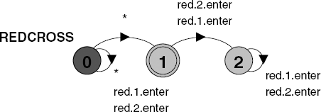
In a parallel composition, * synchronizes the transition it labels with all other transitions in the model, i.e. excluding actions red[1].enter and red[2].enter, but including those labeled by the silent action. It can be seen that the always part of the assertion is captured here by the non-deterministic choice on * which means that at any point in a trace, the automaton can move to state 1.
It could be argued that REDCROSS and BLUECROSS are too weak a specification of the required liveness since they are satisfied if either car 1 or car 2 crosses infinitely often. For example, the properties can be satisfied if car 2 never crosses. This is because, as mentioned previously, a set of actions is treated as a disjunction and so the property REDCROSS is:
assert REDCROSS = []<>(red[1].enter || red[2].enter)A stronger assertion would be:
assertSTRONGRED =forall[i:ID] []<>red[i].enter
Suppose we wished to assert the liveness property that if a car enters the bridge then it should eventually exit. In other words, it does not stop in the middle or fall over the side! We can specify this property for a car as follows:
assert REDEXIT = [](red[1].enter -> <>red[1].exit)The corresponding Büchi automaton (for the negation) is shown in Figure 14.5.
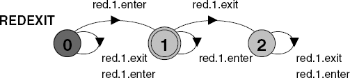
The property holds for both SingleLaneBridge and CongestedBridge. Although cars may not ever enter the congested bridge, if they do enter, they also exit. Consequently, the property is not violated. This is an extremely common form of liveness property which is sometimes termed a "response" property since it is of the form [](request -> <>reply). Note that this form of liveness property cannot be specified using the progress properties of Chapter 7.
In the previous section, we saw the use of the always [] operator to express safety properties and the use of the eventually operator <> to express liveness properties. These represent by far the most common use of linear temporal logic in expressing properties. In the following, we complete the description of our fluent linear temporal logic (FLTL) by describing the remaining operators – until U, weak until W and next time X.
Note
The linear temporal logic formula p U q is true if and only if q is true at the current instant or if q is true at some instant in the future and p is true until that instant.
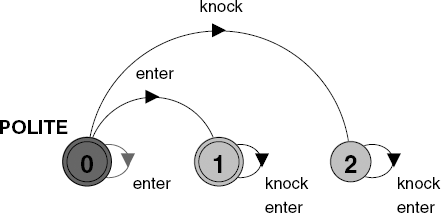
For example, suppose we wish to assert the politeness property of Chapter 7 that we should not enter a room before knocking. We can assert:
assertPOLITE = (!enterUknock)
This asserts both the safety property that we cannot have an enter action before a knock action, and also that a knock action should eventually happen. This can be seen clearly from the Büchi automaton for this property depicted in Figure 14.6. The automaton irretrievably enters the acceptance state 1 if an enter action occurs before a knock action occurs. However, if a knock action never occurs, the property is violated because the automaton remains in state 0 which is also an acceptance state.
Given the until operator, we can state the mutual exclusion property of section 14.2.1 using only action fluents:
assertMUTEX_U = []((p[1].enter -> (!p[2].enterUp[1].exit)) &&(p[2].enter -> (!p[1].enterUp[2].exit)))
This expresses the required mutual exclusion safety property and, in addition, the liveness property that if a process enters the critical section it should eventually exit. However, the property is considerably more complex than that of section 14.2.1 and is difficult to extend to more than two processes.
Note
The linear temporal logic formula p W q is true if and only if either p is true indefinitely or if p U q.
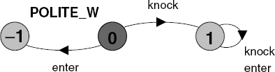
The difference with the previous definition of until is that this definition does not insist that q eventually happens. The formula also holds if p is true indefinitely. This means that if we use weak until for the POLITE property:
assertPOLITE_W = (!enterWknock)
the property becomes a safety property since it no longer requires that knock eventually happens. The safety property is depicted in Figure 14.7.
In the same way, if we replace until with weak until in the definition of the mutex property, it becomes a safety property which generates exactly the same automaton as that depicted in Figure 14.1.
assertMUTEX_W = []((p[1].enter -> (!p[2].enterWp[1].exit)) &&(p[2].enter -> (!p[1].enterWp[2].exit)))
In general, there is no need to distinguish between safety and liveness properties when using FLTL to specify properties. Since the safety check is more efficient than the connected component search used in checking general FLTL properties, the LTSA generates a safety property process if it detects that a property is only a safety property. In fact, determining whether a Büchi automaton can be transformed to a safety property process is non-trivial and the LTSA does not guarantee to perform this transformation for all automata that could be reduced.
It should be noted that we could have specified the liveness property that was included in MUTEX_U in the original MUTEX_N property as follows:
assertEXIT_N =forallforall[i:1..N][](p[i].enter -> <>p[i].exit)assertMUTEX_LIVE = (MUTEX_N && EXIT_N)
MUTEX_LIVE expresses the same property for N processes that MUTEX_U does for two. In fact we can parameterize assertions as follows:
assertMUTEXP(M=2) = []!(exists[i:1..M-1] (CRITICAL[i] && CRITICAL[i+1..M]))assertEXITP(M=2) =forall[i:1..M] [](p[i].enter-> <>p[i].exit)assertMUTEX_LIVEP(P=2) = (MUTEXP(P) && EXITP(P))
We can define the temporal operators always [], eventually <> and weak until W in terms of the until U operator as follows:
<>≡pTrue Up[]≡p! <> !p≡pWq[]p|| (pUq)
In fact, FLTL does not have the explicit constants True and False; instead it permits boolean expressions of constants and parameters. These expressions are termed "rigid", since, unlike fluent propositions, they do not change truth value with the passage of time as measured by the occurrence of events. Thus we can define:
assertTrue =rigid(1)assertFalse =rigid(0)
Rigid expressions can be used in conjunction with parameters and ranges and are essentially used to introduce boolean expressions into FLTL formulae, e.g.
assertEven(V=3) =rigid(V/2 == 0)
By "next instant" in the above definition, we mean when the next action occurs – this includes silent actions. For example, the assertion:
assertSEQ = (a &&Xb &&X Xc)
requires that in the initial instant of system execution the action a occurs followed by the action b, followed by the action c. To check for this sequence, the property process shown in Figure 14.8 is generated:
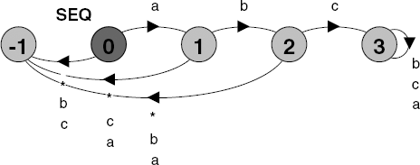
In fact, this form of property is not very useful. If we were to refine or extend our system (using, say, parallel composition and interleaving) such that actions could occur inbetween a, b or c then the property would no longer hold. This is because next time refers to precisely the time at which the next action occurs, whether silent or not. Consequently, it makes finer distinctions than the observational equivalence that is preserved when we minimize processes. As such, it is rarely used in property specification. In addition, it can prohibit the use of partial order reduction, a technique that can dramatically reduce the time taken to check an FLTL property.
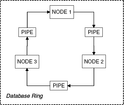
To illustrate the use of logical properties, let us consider a replicated and distributed database where the database nodes are organized in a ring as depicted in Figure 14.9. Communication is uni-directional, occurring clockwise around the ring such that node 1 can send updates to node 2 and receive them from node 3, via communication pipes. Each node of the database can autonomously update its local copy of the data. Updates are circulated round the ring to update other copies. On completion of a cycle, the originator of an update removes it from the ring. When no updates are in progress the copies should be consistent – i.e., all nodes should hold exactly the same data.
Two nodes may perform local updates at the same time and propagate their updates around the ring. This would lead to the situation where nodes receive updates in different orders, leading to inconsistent copies even after all the updates have propagated round the ring. Although we can tolerate copy inconsistency while updates are circulating, we cannot accept inconsistency that persists.
To avoid inconsistency, an update is given a priority depending on its originating node, node i having priority over node j if i<j. Thus an update from node 1 has a higher priority than an update from node 3. In the case of a conflict due to two simultaneous updates, the update from the lower priority node is discarded. A conflict occurs when a node receives an update while still having an outstanding update, which it originated, circulating around the ring.
We can simplify the problem by considering that each database stores only a single data item and by restricting the range of data values that can be stored.
constN = 3// number of nodesrangeNodes = 1..NsetValue = {red, green, blue}
We model the communication between database nodes using the PIPE from section 11.1.1 that models a one-slot buffer:
set S = {[Nodes][Value]}
PIPE  = (put[x:S] -> get[x] -> PIPE).
The updates that circulate round the ring are pairs consisting of the identity of the originating node and the value of the update. For example, [1]['red] is an update from node 1 with the value red. The model for each node is as follows:
NODE(I=0)
       = NODE['null][False],    // initially null value and not updating
     NODE[v:{null,Value}][update:Bool]
       = (when (!update) local[u:Value]      // local update
        -> if (u!=v) then
               (change[u] -> put[I][u] -> NODE[u][True])
            else
               NODE[v][False]
        |get[j:Nodes][u:Value]              // update [j][u]
        -> if (!update) then
               CHANGE(j,u);NODE[u][False]    // update and pass on
            else if  (I==j ) then
               (passive -> NODE[v][False])   // complete update
            else if (i>j) then
               CHANGE(j,u);NODE[u][False]    // priority update
            else
               NODE[v][update]               // discard
        ).

     CHANGE(J=0,U='null)
       = (change[U] -> put[J][U] -> passive ->END).
Whenever a node changes the value of its stored data value, it signals this with the action change[u] and whenever an update is complete the node signals passive. The constants True and False are defined in the usual way:
constFalse = 0constTrue = 1rangeBool = False..True
The composite process for the database ring model is:
||DATABASE_RING
        = (node[i:Nodes]:NODE(i) || pipe[Nodes]:PIPE)
          /{forall[i:Nodes] {
              node[i].put/pipe[i%N+1].put,
              node[i].get/pipe[i].get}
}.Overall, the safety property required of the database model is as follows: when there are no updates in progress, the valuesheldateachnodeshouldbeconsistent. A node that is not engaged in an update signals passive. There can be no updates in progress if all nodes are passive, and the system is said to be quiescent. We can capture the state in which a node is passive by means of the following fluent:
fluent PASSIVE[i:Nodes]
             = <node[i].passive, node[i].change[Value]>
The fluent holds for a node from the time that it signals passive until the time that it signals a change of value. The following assertion captures the quiescent property:
assertQUIESCENT =forall[i:Nodes] PASSIVE[i]
To describe the consistency property, we need to be able to make propositions about the value held by a node as follows:
fluent VALUE[i:Nodes][c:Value]
          = <node[i].change[c],node[i].change[{Value{[c]}}]>
The fluent VALUE is true for a node i and value c if the node has previously changed to the value c and has not yet changed to some other value in the set consisting of Value with c removed. Using this fluent, we can define consistency as the proposition that there exists a value such that each node has that value:
assertCONSISTENT =exists[c:Value]forall[i:Nodes] VALUE[i][c]
The required safety property for the database ring system can now be succinctly expressed by the following assertion, which requires that it is always the case that when the system is quiescent, then it must be consistent.
assert SAFE = [](QUIESCENT -> CONSISTENT)The model we have described does indeed satisfy this property. The reader should replace line 14 of the NODE process with:
else if(/* i>j */ True)then
to obtain an instructive counterexample illustrating the problem of concurrent updates. This modification disables the priority-based conflict resolution in the model.
We have specified the required safety property for the model which ensures that it does not get into a bad state; however, we must also check that the model eventually and repeatedly gets into a good state. The good state for our model is quiescence and the required liveness property is therefore
assert LIVE = []<>QUIESCENTwhich is satisfied by our model.
When a property is satisfied by a model, no further information is returned by the checking tool. The use of FLTL properties gives us the opportunity to generate examples of model executions (traces) which satisfy the property. Such executions are said to be witness executions since they act as a witness to the truth of the property. To generate a witness execution, we simply assert the negation of the property. If the property is satisfied then its negation cannot be satisfied and the LTSA will produce a counterexample trace.
assert WITNESS_LIVE = !LIVEThe above assertion provides the following witness trace for the LIVE property:
Violation of LTL property: @WITNESS_LIVE
     Trace to terminal set of states:
           node.1.local.green
           node.1.change.green
           node.1.put.1.green
           node.2.get.1.green
           node.2.change.green
           node.2.put.1.green
           node.2.passive       PASSIVE.2
           node.2.local.red     PASSIVE.2
           node.3.get.1.green   PASSIVE.2
           node.3.change.green  PASSIVE.2
           node.3.put.1.green   PASSIVE.2
           node.1.get.1.green   PASSIVE.2
node.1.passive PASSIVE.1 && PASSIVE.2
node.3.passive PASSIVE.1 && PASSIVE.2 && PASSIVE.3
Cycle in terminal set:
... ... . .
LTL Property Check in: 281msSome care needs to be taken with witnesses for properties that contain implication. For example, the negation of the safety property SAFE is the property <>(QUIESCENT && !CONSISTENT). We are expecting a counterexample in which quiescence and consistency hold while the tool produces a counterexample in which neither quiescence nor consistency holds, which also violates the property but is not very useful in explaining the operation of the system.
Linear temporal logic is defined for infinite sequences. How do we check FLTL properties for finite executions? In fact, we can easily achieve this by a simple trick in which we add an infinite cycle of an action to the final state. For example, suppose we add the constraint to the database ring that it processes only a single local update:
ONE_UPDATE = (node[Nodes].local[Value] -> END).
     ||DATABASE_RING_ONE = (DATABASE_RING || ONE_UPDATE).
To permit the FLTL properties to be checked against this modified system, we change the constraint to:
ONE_UPDATE = (node[Nodes].local[Value] -> ENDED),
     ENDED      = (ended -> ENDED).
The properties LIVE and SAFE hold for the systems and the following witness execution can be produced for SAFE:
Violation of LTL property: @WITNESS_SAFE
     Trace to terminal set of states:
           node.1.local.blue
           node.1.change.blue  VALUE.1.blue
           node.1.put.1.blue   VALUE.1.blue
           node.2.get.1.blue   VALUE.1.blue
           node.2.change.blue  VALUE.1.blue && VALUE.2.blue
           node.2.put.1.blue   VALUE.1.blue && VALUE.2.blue
           node.2.passive      PASSIVE.2
                            && VALUE.1.blue && VALUE.2.blue
           node.3.get.1.blue   PASSIVE.2
                            && VALUE.1.blue && VALUE.2.blue
node.3.change.blue PASSIVE.2
&& VALUE.1.blue && VALUE.2.blue && VALUE.3.blue
node.3.put.1.blue PASSIVE.2
&& VALUE.1.blue && VALUE.2.blue && VALUE.3.blue
node.1.get.1.blue PASSIVE.2
&& VALUE.1.blue && VALUE.2.blue && VALUE.3.blue
node.1.passive PASSIVE.1 && PASSIVE.2
&& VALUE.1.blue && VALUE.2.blue && VALUE.3.blue
node.3.passive PASSIVE.1 && PASSIVE.2 && PASSIVE.3
&& VALUE.1.blue && VALUE.2.blue && VALUE.3.blue
Cycle in terminal set:
ended PASSIVE.1 && PASSIVE.2 && PASSIVE.3
&& VALUE.1.blue && VALUE.2.blue && VALUE.3.blue
LTL Property Check in: 31msThe primitive propositions of the linear temporal logic we described in this chapter are termed "fluents". A fluent is defined by a set of initiating actions and a set of terminating actions. At a particular instant, a fluent is true if and only if it was initially true or an initiating action has previously occurred and, in both cases, no terminating action has yet occurred. Using fluents, we can map the trace produced by a model into a sequence of sets. Each set in the sequence contains the fluents that are true at the point the corresponding action in the trace occurs. Fluent linear temporal logic (FLTL) is defined with respect to these sequences. For each action, we define a synonymous fluent which holds when the action occurs and becomes false immediately the following action occurs. We termed these actions "fluents" and they can be freely mixed with explicitly defined fluents in expressions. The following table summarizes the temporal operators used in FLTL ("iff" abbreviates "if and only if"):
next time | iff |
always | iff |
eventually | iff |
until | iff |
weak until | iff |
The chapter outlined some typical ways of expressing safety and liveness properties. Using the database ring example, we also explained how to produce witness executions and how to deal with finite executions. In checking liveness properties, we make the same assumptions with respect to fair choice as those made in Chapter 7 and use the same action priority approach to generate adverse scheduling conditions.
In Chapter 7, we mentioned that the general LTL model-checking procedure – that of translating the negation of the required LTL formula into a Büchi automaton, composing this automaton with the target model and then searching for connected components containing acceptance states – is due to Gribomont and Wolper (1989). We also mentioned that this technique has found widespread usage in the SPIN model checker (Holtzmann, 1991, 1997). Indeed, as far as possible, we have followed the syntax of LTL formulae used in SPIN. The use of fluents in the context of LTL model checking is due to Giannakopoulou and Magee (2003) and the component used in the LTSA to translate LTL formulae into Büchi automata is due to Giannakopoulou and Lerda (2002). A version of FLTL for specifying the properties of the timed models of Chapter 12 can be found in Letier, Kramer, Magee, et al. (2005). The term "fluent" originally comes from the time-varying quantity in Newton's calculus but has more recently been adopted by the Artificial Intelligence community with a meaning consistent with the one used here (Sandewall, 1995).
Most properties specified in LTL conform to a restricted set of forms or patterns. A set of patterns used in specifying properties has been codified by Dwyer, Avrunin and Corbett (1999). These patterns are coded in a number of formalisms that include linear temporal logic and computation tree logic (CTL). While LTL is defined with respect to infinite execution sequences or linear time, CTL is a temporal logic defined with respect to a branching tree of execution paths or branching time. CTL was used in the model-checking work originated by Clarke, Emerson and Sistla (1986). There has been much academic debate on the relative advantages of LTL and CTL, starting with the classic paper by Lamport (1980) entitled ''Sometime" Is Sometimes "Not Never": On the Temporal Logic of Programs to the more recent Branching vs. Linear Time: Final Showdown by Vardi (2001). Pnueli (1977) was responsible for the original idea of using temporal logic as the logical basis for proving correctness properties of concurrent programs.
Finally, it should be noted that the database ring is due to Bill Roscoe (1998). The example, which was used to illustrate an approach to modeling change in the form of safe node deletion and creation, appears in a paper by Kramer and Magee (1998).
14.1 Using FLTL, specify and check the exclusion safety properties for neighbors in the Dining Philosophers problem of Chapter 6. In addition, specify and check the liveness properties, including the response property that ensures that if a philosopher is hungry, he will eventually eat. Use witnesses to provide examples of property satisfaction.
14.2 Using FLTL, specify safety and liveness properties for the Readers–Writers problem of section 7.5. Check that these give the same results as the corresponding properties specified in Chapter 7 and for the same properties used in the verification models of Chapter 13.
14.3 Using FLTL, specify and check the exclusion safety properties for the warring neighbors of exercise 7.6, and for Peterson's Algorithm for two processes of exercise 7.7. In addition, specify and check the liveness properties, including the response property that ensures that if a neighbor wants to enter the field, he will eventually gain exclusive access. Use witnesses to provide examples of property satisfaction.
14.4 Using FLTL, specify safety and liveness properties for the cruise control system of Chapter 8. Check these properties against the model of Chapter 8. (Hint: define fluents for each of the abstract states – active, cruising, enabled, etc. – as necessary.)
14.5 Using FLTL, specify a safety property to replace the property
SAFEspecified in section 11.3.1 for the Announcer–Listener system. (Hint: define a fluent which holds when a process registers for a pattern and note that a separateSAFEprocess is created in Chapter 11 for each listener process.)