
The execution of a concurrent program consists of multiple processes active at the same time. As discussed in the last chapter, each process is the execution of a sequential program. A process progresses by submitting a sequence of instructions to a processor for execution. If the computer has multiple processors then instructions from a number of processes, equal to the number of physical processors, can be executed at the same time. This is sometimes referred to as parallel or real concurrent execution. However, it is usual to have more active processes than processors. In this case, the available processors are switched between processes. Figure 3.1 depicts this switching for the case of a single processor supporting three processes, A, B and C. The solid lines represent instructions from a process being executed on the processor. With a single processor, each process makes progress but, as depicted in Figure 3.1, instructions from only one process at a time can be executed.
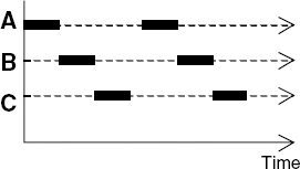
The switching between processes occurs voluntarily or in response to interrupts. Interrupts signal external events such as the completion of an I/O operation or a clock tick to the processor. As can be seen from Figure 3.1, processor switching does not affect the order of instructions executed by each process. The processor executes a sequence of instructions which is an interleaving of the instruction sequences from each individual process. This form of concurrent execution using interleaving is sometimes referred to as pseudo-concurrent execution since instructions from different processes are not executed at the same time but are interleaved. We use the terms parallel and concurrent interchangeably and usually do not distinguish between real and pseudo-concurrent execution since, in general, the same programming principles and techniques are applicable to both physically (real) concurrent and interleaved execution. In fact, we always model concurrent execution as interleaved whether or not implementations run on multiple processors.
This chapter describes how programs consisting of multiple processes are modeled and illustrates the correspondence between models and implementations of concurrent programs by a multi-threaded Java example.
In the previous chapter, we modeled a process abstractly as a state machine that proceeds by executing atomic actions, which transform its state. The execution of a process generates a sequence (trace) of atomic actions. We now examine how to model systems consisting of multiple processes.
The first issue to consider is how to model the speed at which one process executes relative to another. The relative speed at which a process proceeds depends on factors such as the number of processors and the scheduling strategy – how the operating system chooses the next process to execute. In fact, since we want to design concurrent programs which work correctly independently of the number of processors and the scheduling strategy, we choose not to model relative speed but state simply that processes execute at arbitrary relative speeds. This means that a process can take an arbitrarily long time to proceed from one action to the next. We abstract away from execution time. This has the disadvantage that we can say nothing about the real-time properties of programs but has the advantage that we can verify other properties independently of the particular configuration of the computer and its operating system. This independence is clearly important for the portability of concurrent programs.
The next issue is how to model concurrency or parallelism. Is it necessary to model the situation in which actions from different processes can be executed simultaneously by different processors in addition to the situation in which concurrency is simulated by interleaved execution? We choose always to model concurrency using interleaving. An action a is concurrent with another action b if a model permits the actions to occur in either the order a → b or the order b → a. Since we do not represent time in the model, the fact that the event a actually occurs at the same time as event b does not affect the properties we can assert about concurrent executions.
Finally, having decided on an interleaved model of concurrent execution, what can we say about the relative order of actions from different processes in the interleaved action trace representing the concurrent program execution? We know that the actions from the same process are executed in order. However, since processes proceed at arbitrary relative speeds, actions from different processes are arbitrarily interleaved. Arbitrary interleaving turns out to be a good model of concurrent execution since it abstracts the way processors switch between processes as a result of external interrupts. The timing of interrupts relative to process execution cannot in general be predetermined since actions in the real world cannot be predicted exactly – we cannot foretell the future.
The concurrent execution model in which processes perform actions in an arbitrary order at arbitrary relative speeds is referred to as an asynchronous model of execution. It contrasts with the synchronous model in which processes perform actions in simultaneous execution steps, sometimes referred to as lock-step.
Note
If P and Q are processes then (P||Q) represents the concurrent execution of P and Q. The operator || is the parallel composition operator.
Parallel composition yields a process, which is represented as a state machine in the same way as any other process. The state machine representing the composition generates all possible interleavings of the traces of its constituent processes. For example, the process:
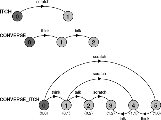
ITCH = (scratch->STOP).
has a single trace consisting of the action scratch. The process:
CONVERSE = (think->talk->STOP).
has the single trace think→talk. The composite process:
||CONVERSE_ITCH = (ITCH || CONVERSE).
has the following traces:
think→talk→scratch
     think→scratch→talk
     scratch→think→talk
The state machines corresponding to ITCH, CONVERSE and CONVERSE_ITCH are depicted in Figure 3.2. The state machine representing the composition is formed by the Cartesian product of its constituents. For example, if ITCH is in state(i) and CONVERSE is in state (j), then this combined state is represented by CONVERSE_ITCH in state (<i, j>). So if CONVERSE has performed the think action and is in state (1) and ITCH performs its scratch action and is in state (1) then the state representing this in the composition is state (< 1,1>). This is depicted as state (4) of the composition. We do not manually compute the composite state machines in the rest of the book, since this would be tedious and error-prone. Compositions are computed by the LTSA tool and the interested reader may use it to verify that the compositions depicted in the text are in fact correct.
From Figure 3.2, it can be seen that the action scratch is concurrent with both think and talk as the model permits these actions to occur in any order while retaining the constraint that think must happen before talk.Inotherwords, one must think before talking but one can scratch at any point!
Composite process definitions are always preceded by || to distinguish them from primitive process definitions. As described in the previous chapter, primitive processes are defined using action prefix and choice while composite processes are defined using only parallel composition. Maintaining this strict distinction between primitive and composite processes is required to ensure that the models described by FSP are finite.
As a further example, the following processes model a clock radio which incorporates two independent activities: a clock which ticks and a radio which can be switched on and off. The state machine for the composition is depicted in Figure 3.3.
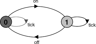
CLOCK = (tick->CLOCK).
     RADIO = (on->off->RADIO).

     ||CLOCK_RADIO = (CLOCK || RADIO).
Examples of traces generated by the state machine of Figure 3.3 are given below. The LTSA Animator can be used to generate such traces.
on→tick→tick→off→tick→tick→tick→on→off→...
     tick→on→off→on→off→on→off→tick→on→tick→...
The parallel composition operator obeys some simple algebraic laws:
Commutative:(P||Q) = (Q||P)Associative:(P||(Q||R)) = ((P||Q)||R) = (P||Q||R).
Taken together these mean that the brackets can be dispensed with and the order that processes appear in the composition is irrelevant.
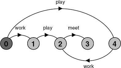
The examples in the previous section are all compositions of processes with disjoint alphabets. That is, the processes in a composition do not have any actions in common. If processes in a composition do have actions in common, these actions are said to be shared. Shared actions are the way that process interaction is modeled. While unshared actions may be arbitrarily interleaved, a shared action must be executed at the same time by all the processes that participate in that shared action. The following example is a composition of processes that share the action meet.
BILL = (play -> meet -> STOP).
     BEN  = (work -> meet -> STOP).

     ||BILL_BEN = (BILL || BEN).
The possible execution traces of the composition are:
play→work→meet
     work→play→meet
The unshared actions, play and work, are concurrent and thus may be executed in any order. However, both of these actions are constrained to happen before the shared action meet. The shared action synchronizes the execution of the processes BILL and BEN. The state machine for the composite process is depicted in Figure 3.4.
The next example consists of a process that manufactures an item and then signals that the item is ready for use by a shared ready action. A user can only use the item after the ready action occurs.
MAKER = (make->ready->MAKER).
     USER  = (ready->use->USER).

     ||MAKER_USER = (MAKER || USER).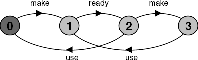
From Figure 3.5, it can be seen that the following are possible execution traces:
make→ready→use→make→ready→...
     make→ready→make→use→ready→...
After the initial item is manufactured and becomes ready, manufacture and use can proceed in parallel since the actions make and use can occur in any order. However, it is always the case that an item is made beforeit is used since the first action is make in all traces. The second trace shows that two items can be made before the first is used. Suppose that this is undesirable behavior and we do not wish the MAKER process to get ahead in this way. The solution is to modify the model so that the user indicates that the item is used. This used action is shared with the MAKER who now cannot proceed to manufacture another item until the first is used. This second version is shown below and in Figure 3.6.
MAKERv2 = (make->ready->used->MAKERv2).
     USERv2  = (ready->use->used->USERv2).

     ||MAKER_USERv2 = (MAKERv2 || USERv2).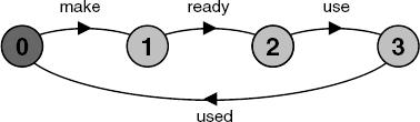
The interaction between MAKER and USER in this second version is an example of a handshake, an action which is acknowledged by another. As we see in the chapters to follow, handshake protocols are widely used to structure interactions between processes. Note that our model of interaction does not distinguish which process instigates a shared action even though it is natural to think of the MAKER process instigating the ready action and the USER process instigating the used action. However, as noted previously, an output action instigated by a process does not usually form part of a choice while an input action may.
The examples of synchronization so far are between two processes; however, many processes can engage in a shared action. The next example illustrates the use of multi-party synchronization in a small manufacturing system which produces two different parts and assembles the parts into a product. Assembly cannot take place until both parts are ready. Again, makers are not permitted to get ahead of users. The state machine is depicted in Figure 3.7.
MAKE_A   = (makeA->ready->used->MAKE_A).
     MAKE_B   = (makeB->ready->used->MAKE_B).
     ASSEMBLE = (ready->assemble->used->ASSEMBLE).

     ||FACTORY = (MAKE_A || MAKE_B || ASSEMBLE).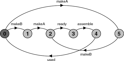
Since a parallel composition of processes is itself a process, called a composite process, it can be used in the definition of further compositions. We can restructure the previous example by creating a composite process from MAKE_A and MAKE_B as follows:
MAKE_A = (makeA->ready->used->MAKE_A).
     MAKE_B = (makeB->ready->used->MAKE_B).

     ||MAKERS = (MAKE_A || MAKE_B).
The rest of the factory description now becomes:
ASSEMBLE = (ready->assemble->used->ASSEMBLE).

     ||FACTORY = (MAKERS || ASSEMBLE).
The state machine remains that depicted in Figure 3.7. Substituting the definition for MAKERS in FACTORY and applying the commutative and associative laws for parallel composition stated in the last section results in the original definition for FACTORY in terms of primitive processes. The LTSA tool can also be used to confirm that the same state machine results from the two descriptions.
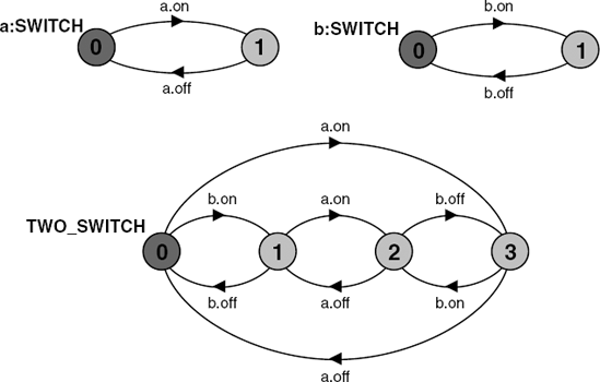
Given the definition of a process, we often want to use more than one copy of that process in a program or system model. For example, given the definition for a switch:
SWITCH = (on->off->SWITCH).
we may wish to describe a system that is the composition of two distinct switches. However, if we describe this system as (SWITCH||SWITCH), the composition is indistinguishable from a single switch since the two switch processes synchronize on their shared actions on and off. We must ensure that the actions of each SWITCH process are not shared, i.e. they must have disjoint labels. To do this we use the process labeling construct.
Note
a:P prefixes each action label in the alphabet of P with the label "a".
A system with two switches can now be defined as:
||TWO_SWITCH = (a:SWITCH || b:SWITCH).
The state machine representation for the processes a:SWITCH and b:SWITCH is given in Figure 3.8. It is clear that the alphabets of the two processes are disjoint, i.e. {a.on, a.off} and {b.on, b.off}.
Using a parameterized composite process, SWITCHES, we can describe an array of switches in FSP as follows:
||SWITCHES(N=3) =(forall[i:1..N] s[i]:SWITCH).An equivalent but shorter definition is:
||SWITCHES(N=3) =(s[i:1..N]:SWITCH).
Processes may also be labeled by a set of prefix labels. The general form of this prefixing is as follows:
Note
{a1,..,ax}::P replaces every action label n in the alphabet of P with the labels a1.n,...,ax.n. Further, every transition (n->Q) in the definition of P is replaced with the transitions ({a1.n,...,ax.n}->Q).
We explain the use of this facility in the following example. The control of a resource is modeled by the following process:
RESOURCE = (acquire->release->RESOURCE).
and users of the resource are modeled by the process:
USER = (acquire->use->release->USER).
We wish to model a system consisting of two users that share the resource such that only one user at a time may be using it (called "mutual exclusion"). The two users may be modeled using process labeling as a:USER and b:USER. This means that there are two distinct actions (a.acquire and b.acquire) toobtaintheresource and similarly two actions to free it (a.release and b.release). Consequently, RESOURCE must be labeled with the set {a,b} to yield these transitions. The composition is described below.
||RESOURCE_SHARE =
           (a:USER || b:USER || {a,b}::RESOURCE).
The state machine representations of the processes in the RESOURCE_SHARE model are depicted in Figure 3.9. The effect of process labeling on RESOURCE can be clearly seen. The composite process graph shows that the desired result of allowing only one user to use the resource at a time has been achieved.
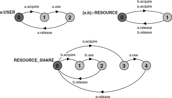
A perceptive reader might notice that our model of the RESOURCE alone would permit one user to acquire the resource and the other to release it! For example, it would permit the following trace:
a.acquire →b.release →...
However, each of the USER processes cannot release the resource until it has succeeded in performing an acquire action. Hence, when the RESOURCE is composed with the USER processes, this composition ensures that only the same user that acquired the resource can release it. This is shown in the composite process RESOURCE_SHARE in Figure 3.9. This can also be confirmed using the LTSA Animator to run through the possible traces.
Note
Relabeling functions are applied to processes to change the names of action labels. The general form of the relabeling function is:
/{newlabel_1/oldlabel_1,... newlabel_n/oldlabel_n}.Relabeling is usually done to ensure that composite processes synchronize on the desired actions. A relabeling function can be applied to both primitive and composite processes. However, it is generally used more often in composition.
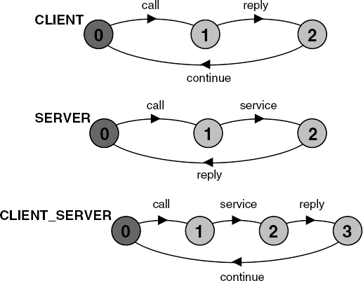
A server process that provides some service and a client process that invokes the service are described below:
CLIENT = (call->wait->continue->CLIENT).
     SERVER = (request->service->reply->SERVER).
As described, the CLIENT and SERVER have disjoint alphabets and do not interact in any way. However, using relabeling, we can associate the call action of the CLIENT with the request action of the SERVER and similarly the reply and wait actions. The composition is defined below.
||CLIENT_SERVER = (CLIENT || SERVER)
                       /{call/request, reply/wait}.
The effect of applying the relabeling function can be seen in the state machine representations of Figure 3.10. The label call replaces request in the description of SERVER and reply replaces wait in the description of CLIENT.
An alternative formulation of the client–server system is described below using qualified or prefixed labels.
SERVERv2 = (accept.request
                ->service->accept.reply->SERVERv2).
     CLIENTv2 = (call.request
                ->call.reply->continue->CLIENTv2).

     ||CLIENT_SERVERv2 = (CLIENTv2 || SERVERv2)
                         /{call/accept}.
The relabeling function /{call/accept} replaces any label prefixed by accept with the same label prefixed by call. Thus accept.request becomes call.request and accept.reply becomes call.reply in the composite process CLIENT_SERVERv2. This relabeling by prefix is useful when a process has more than one interface. Each interface consists of a set of actions and can be related by having a common prefix. If required for composition, interfaces can be relabeled using this prefix as in the client–server example.
Note
When applied to a process P, the hiding operator {a1..ax} removes the action names a1..ax from the alphabet of P and makes these concealed actions "silent". These silent actions are labeled tau. Silent actions in different processes are not shared.
The hidden actions become unobservable in that they cannot be shared with another process and so cannot affect the execution of another process. Hiding is essential in reducing the complexity of large systems for analysis purposes since, as we see later, it is possible to minimize the size of state machines to remove tauactions. Hiding can be applied to both primitive and composite processes but is generally used in defining composite processes. Sometimes it is more convenient to state the set of action labels which are visible and hide all other labels.
Note
When applied to a process P, the interface operator @{a1..ax} hides all actions in the alphabet of P not labeled in the set a1..ax.
The following definitions lead to the state machine depicted in Figure 3.11:
USER = (acquire->use->release->USER)
            {use}.

     USER = (acquire->use->release->USER)
            @{acquire,release}.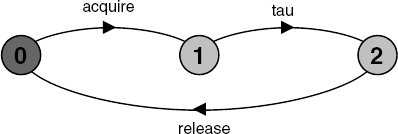
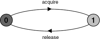
Minimization of USER removes the hidden tau action to produce a state machine with equivalent observable behavior, but fewer states and transitions (Figure 3.12). LTSA can be used to confirm this.
We have used state machine diagrams to depict the dynamic behavior of processes. State machine diagrams represent the dynamic process operators, action prefix and choice. However, these diagrams do not capture the static structure of a model. While the result of applying parallel composition can be described as a state machine (since it is a process), the parallel composition expression itself is not represented. Parallel composition, relabeling and hiding are static operators that describe the structure of a model in terms of primitive processes and their interactions. Composition expressions can be represented graphically as shown in Figure 3.13.
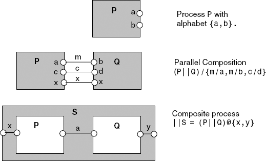
A process is represented as a box with visible actions shown as circles on the perimeter. A shared action is depicted as a line connecting two action circles, with relabeling if necessary. A line joining two actions with the same name indicates only a shared action since relabeling is not required. A composite process is the box enclosing a set of process boxes. The alphabet of the composite is again indicated by action circles on the perimeter. Lines joining these circles to internal action circles show how the composite's actions are defined by primitive processes. These lines may also indicate relabeling functions if the composite name for an action differs from the internal name. Those actions that appear internally, but are not joined to a composite action circle, are hidden. This is the case for action a inside S in Figure 3.13. The processes inside a composite may, of course, themselves be composite and have structure diagram descriptions.
We sometimes use a line in a structure diagram to represent a set of shared actions that have a common prefix label. The line is labeled with the prefix rather than explicitly by the actions. The example in Figure 3.14 uses the single-slot buffer of section 2.1.3 to construct a buffer that can store two values. A definition of the single-slot buffer is given below.
range T = 0..3
BUFF = (in[i:T]->out[i]->BUFF).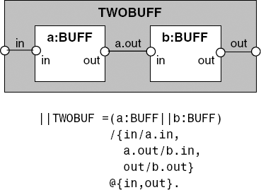
Each of the labels in the diagram of Figure 3.14 – in, out and a.out – represents the set of labels in[i:T], out[i:T] and a.out[i:T], respectively.
Sometimes we omit the label on a connection line where it does not matter how relabeling is done since the label does not appear in the alphabet (interface) of the composite. For example, in Figure 3.14, it would not matter if we omitted the label a.out and used b.in/a.out instead of a.out/b.in as shown. We also omit labels where all the labels are the same, i.e. no relabeling function is required.
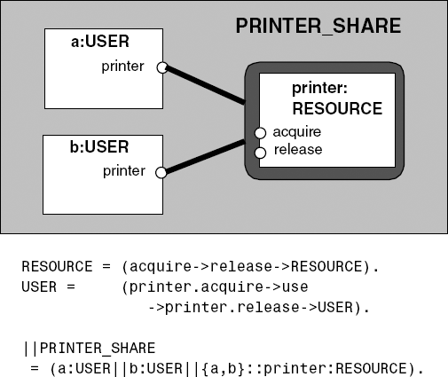
Lastly, we use a diagrammatic convention to depict the common situation of resource sharing as described in section 3.1.3. The resource-sharing model is repeated in Figure 3.15 together with its structure diagram representation. The resource is not anonymous as before; it is named printer. Sharing is indicated by enclosing a process in a rounded rectangle. Processes, which share the enclosed process, are connected to it by thick lines. The lines in Figure 3.15 could be labeled a.printer and b.printer; however these labels are omitted as a relabeling function is not required.
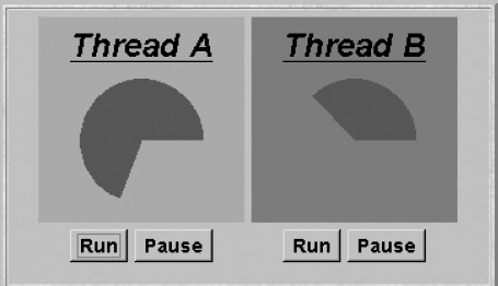
Concurrency occurs in Java programs when more than one thread is alive. Remember from Chapter 2 that a thread is alive if it has started but has not yet terminated. In this section, we present an example of a simple Java multi-threaded program that has two concurrently active threads in addition to the main thread of execution present in every Java program. The threads in the example program do not interact directly. The topic of how threads interact is left to succeeding chapters.
The example program drives the display depicted in Figure 3.16. Each of the threads, A and B, can be run and paused by pressing the appropriate button. When a thread is run, the display associated with it rotates. Rotation stops when the thread is paused. When a thread is paused, its background color is set to red and when it is running, the background color is set to green. The threads do not interact with each other; however they do interact with the Java main thread of execution when the buttons are pressed.
The behavior of each of the two threads in the applet is modeled by the following ROTATOR process:
ROTATOR = PAUSED,
     PAUSED  = (run->RUN | pause->PAUSED),
     RUN     = (pause->PAUSED |{run,rotate}->RUN).
The process cannot perform the rotate action until it moves into the RUN state. This can only occur after the run action, which models pushing the Run button. When the pause action occurs – modeling the Pause button – the process moves back to the PAUSED state in which the rotate action cannot take place. The model implies that the implementation of ROTATOR runs forever – there is no way of stopping it. It is not good practice to program threads which run forever; they should terminate in an orderly manner when, for example, the Applet.stop() method is called by a browser. As we discussed in the previous chapter, the designers of Java do not recommend using Thread.stop() to terminate the execution of a thread. Instead, they suggest the use of Thread.interrupt() which raises the InterruptedException that allows a thread to clean up before terminating. We can include termination in the ROTATOR process as shown below. The corresponding LTS is depicted in Figure 3.17.
ROTATOR = PAUSED,
     PAUSED  = (run->RUN |pause->PAUSED
               |interrupt->STOP),
     RUN     = (pause->PAUSED |{run,rotate}->RUN
               |interrupt->STOP).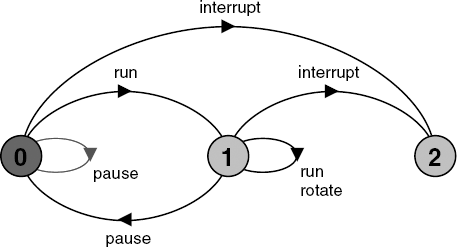
This revised model includes the effect of an interrupt action. Whether the ROTATOR process is in the paused or running state, the interrupt takes it into a final state in which no further actions are possible, i.e. it is terminated. The model for the ThreadDemo program consisting of two copies or instances of the ROTATOR thread is shown in Figure 3.18.
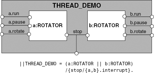
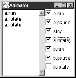
We have relabeled the a.interrupt and b.interrupt actions to be the same action stop, indicating that we always interrupt both threads at the same time, when the browser calls Applet.stop(). Having constructed the model, we can animate it using the LTSA tool to check that its behavior corresponds to the behavior we expect of the ThreadDemo applet. Figure 3.19 shows a screen shot of the LTSA Animator window. As described in Chapter 2, those actions that can be chosen for execution are ticked. In the figure, the action a.run has put process a in the state where a.rotate actions can occur while process b cannot perform its b.rotate action since b.run has not occurred.
In fact, in the implementation, the environment is provided by the main thread of execution of the Java program. We can of course also model this main thread as a process that shares the actions. The display can rotate at any time and the buttons can be pushed at any time. Consequently, this main thread can be modeled as:
MAIN = ({a.rotate,a.run,a.pause,stop,
              b.rotate,b.run,b.pause}->MAIN).
Composing MAIN with THREAD_DEMO does not modify the behavior of THREAD_DEMO since it does not provide any additional ordering constraints on the actions.
The implementation for the process is provided by the Rotator class, which implements the Runnable interface as shown in Program 3.1. The run() method simply finishes if an InterruptedException raised by Thread.interrupt() occurs. As described in the previous chapter, when the run() method exits, the thread which is executing it terminates.
Example 3.1. Rotator class.
classRotatorimplementsRunnable {publicvoid run() {try{while(true) ThreadPanel.rotate(); }catch(InterruptedException e) {} } }
The details of suspending and resuming threads when buttons are pressed are encapsulated in the ThreadPanel class. The run() method simply calls Thread-Panel.rotate() to move the display. If the Pause button has been pressed, this method suspends a calling thread until Run is pressed. We use the ThreadPanel class extensively in programs throughout the book. The methods offered by this class relevant to the current example are listed in Program 3.2.
The ThreadPanel class manages the display and control buttons for the thread that is created by a call to the start() method. The thread is created from the class DisplayThread which is derived from Thread. The implemention of start() is given below:
Example 3.2. ThreadPanel class.
public classThreadPanelextendsPanel {// construct display with title and segment color cpublicThreadPanel(String title, Color c) {...}// rotate display of currently running thread 6 degrees// return value not used in this examplepublic staticboolean rotate()throwsInterruptedException {...}// create a new thread with target r and start it runningpublicvoid start(Runnable r) {...}// stop the thread using Thread.interrupt()publicvoid stop() {...} }
publicvoid start(Runnable r) { thread =newDisplayThread(canvas,r,...); thread.start(); }
where canvas is the display used to draw the rotating segment. The thread is terminated by the stop() method using Thread.interrupt() as shown below:
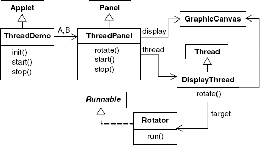
public void stop() {thread.interrupt();}ThreadPanel delegates calls to rotate() to DisplayThread. The relationship between these classes, the applet and the Rotator class is depicted in the class diagram of Figure 3.20. Note that rotate() is a static method which determines the particular thread instance to which it applies by calling the method Thread.currentThread(). This returns a reference to the currently running thread, which, of course, is the only thread which can have called the method.
The Applet class ThreadDemo creates the two ThreadPanel displays when it is initialized and the two threads when it is started. The class is listed in Program 3.3.
In section 2.2.3, we saw that Java provides a standard set of operations on threads including suspend() and resume() which the reader might surmise have been used to suspend and resume the execution of the threads in response to pushing the buttons. In fact, we cannot use the operations directly in the implementation of the ThreadDemo program for the following reason. The rotate() method acquires and releases resources from the graphical interface provided by the browser in which the applet runs. If we used suspend(), a thread could be suspended at some arbitrary time when Pause was pressed. In particular, it could be suspended while it was holding on to display resources. This can cause some browsers to hang or deadlock[1]. Consequently, the threads in the program are suspended using the methods Object.wait() and Object.notify(). We defer an explanation of how these work until Chapter 5 and consider the problem of deadlock in Chapter 6.
Example 3.3. ThreadDemo applet class.
public classThreadDemoextendsApplet { ThreadPanel A; ThreadPanel B;publicvoid init() { A = new ThreadPanel("Thread A",Color.blue); B = new ThreadPanel("Thread B",Color.blue); add(A); add(B); }publicvoid start() { A.start(newRotator()); B.start(newRotator()); }publicvoid stop() { A.stop(); B.stop(); } }
This chapter has introduced the concept of interleaving both as a way of executing multiple processes on a single processor and as a way of modeling concurrent execution. The chapter has dealt mainly with modeling concurrency:
The model of concurrency is interleaved and asynchronous. By asynchronous we mean that processes proceed at arbitrary relative speeds and consequently their actions can be arbitrarily interleaved.
The parallel composition of two or more processes modeled as finite state processes results in a finite state process that can generate all possible interleavings of the execution traces of the constituent processes.
Process interaction is modeled by shared actions, where a shared action is executed at the same time by all the processes that share the action. A shared action can only occur when all the processes that have the action in their alphabets are ready to participate in it – they must all have the action as an eligible choice.
Process labeling, relabeling and hiding are all ways of describing and controlling the actions shared between processes. Minimization can be used to help reduce the complexity of systems with hidden actions.
Parallel composition and the labeling operator describe the static structure of a model. This structure can be represented diagrammatically by structure diagrams.
Concurrent execution in Java is programmed simply by creating and starting multiple threads.
The parallel composition operator used here is from CSP (Hoare, 1985). It is also used in the ISO specification language LOTOS (ISO/IEC, 1988). We have chosen to use explicit process labeling as the sole means of creating multiple copies of a process definition. LOTOS and CSP introduce the interleaving operator "|||" which interleaves all actions even if they have the same name. We have found that explicit process labeling clarifies trace information from the LTSA tool. Further, having a single composition operator rather than the three provided by LOTOS is a worthwhile notational simplification. The simple rule that actions with the same name synchronize and those that are different interleave is intuitive for users to grasp.
Most process calculi have an underlying interleaved model of concurrent execution. The reader should look at the extensive literature on Petri Nets (Peterson, J.L., 1981) for a model that permits simultaneous execution of concurrent actions.
Forms of action relabeling and hiding are provided in both CSP (Hoare, 1985) and CCS (Milner, 1989). The FSP approach is based on that of CCS, from which the concepts of the silent tau action and observational equivalence also come. Techniques for equivalence testing and minimization can be found in the paper by Kanellakis and Smolka (1990).
The structure diagrams presented in this chapter are a simplified form of the graphical representation of Darwin (Magee, Dulay and Kramer, 1994; Magee, Dulay, Eisenbach et al., 1995), a language for describing Software Architectures. The Darwin toolset includes a translator from Darwin to FSP composition expressions (Magee, Kramer and Giannakopoulou, 1997).
Exercises 3.1 to 3.6 are more instructive and interesting if the FSP models are developed using the analyzer tool LTSA.
3.1 Show that
S1andS2describe the same behavior:P = (a->b->P). Q = (c->b->Q). ||S1 = (P||Q). S2 =(a->c->b->S2| c->a->b->S2).3.2
ELEMENT=(up->down->ELEMENT)accepts anupaction and then adownaction. Using parallel composition and theELEMENTprocess describe a model that can accept up to fourupactions before adownaction. Draw a structure diagram for your solution.3.3 Extend the model of the client–server system described in section 3.1.4 such that more than one client can use the server.
3.4 Modify the model of the client–server system in exercise 3.3 such that the call may terminate with a timeout action rather than a response from the server. What happens to the server in this situation?
3.5 A roller-coaster control system only permits its car to depart when it is full. Passengers arriving at the departure platform are registered with the roller-coaster controller by a turnstile. The controller signals the car to depart when there are enough passengers on the platform to fill the car to its maximum capacity of M passengers. The car goes around the roller-coaster track and then waits for another M passengers. A maximum of M passengers may occupy the platform. Ignore the synchronization detail of passengers embarking from the platform and car departure. The roller coaster consists of three processes:
TURNSTILE, CONTROLandCAR. TURNSTILEandCONTROLinteract by the shared actionpassengerindicating an arrival andCONTROLandCARinteract by the shared actiondepartsignaling car departure. Draw the structure diagram for the system and provide FSP descriptions for each process and the overall composition.3.6 A museum allows visitors to enter through the east entrance and leave through its west exit. Arrivals and departures are signaled to the museum controller by the turnstiles at the entrance and exit. At opening time, the museum director signals the controller that the museum is open and then the controller permits both arrivals and departures. At closing time, the director signals that the museum is closed, at which point only departures are permitted by the controller. Given that it consists of the four processes
EAST, WEST, CONTROLandDIRECTOR, draw the structure diagram for the museum. Now provide an FSP description for each of the processes and the overall composition.3.7 Modify the example Java program of section 3.2.2 such that it consists of three rotating displays.