![]()
Handling Live Data with D3
In this chapter you will see how to develop real-time charts using the D3 library. Indeed, you will create a line chart that displays the real-time values generated from a function that simulates an external source of data. The data will be generated continuously, and therefore the line chart will vary accordingly, always showing the latest situation.
In the second part of this chapteryou will develop a chart that is slightly more complex. This time, you will be using an example in which the data source is a real database. First, you will implement a line chart that will read the data contained in an external file. Later, you will learn how to use the example to read the same data, but this time from the table of a database.
Real-Time Charts
You have a data source that simulates a function that returns random variations on the performance of a variable. These values are stored in an array that has the functions of a buffer, in which you want to contain only the ten most recent values. For each input value that is generated or acquired, the oldest one is replaced with the new one. The data contained in this array are displayed as a line chart that updates every 3 seconds. Everything is activated by clicking a button.
Let us start setting the bases to represent a line chart (to review developing line charts with the D3 library, see Chapter 3). First, you write the HTML structure on which you will build your chart, as shown in Listing 9-1.
Listing 9-1. Ch9_01.html
<!DOCTYPE html>
<html>
<head>
<meta charset="utf-8">
<script src="http://d3js.org/d3.v3.js"></script>
<style>
    //add the CSS styles here
</style>
<body>
<script type="text/javascript">
    // add the JavaScript code here
</script>
</body>
</html>
Now, you start to define the variables that will help you during the writing of the code, beginning with the management of the input data. As previously stated, the data that you are going to represent on the chart come from a function that generates random variations, either positive or negative, from a starting value. You decide to start from 10.
So, starting from this value, you receive from the random function a sequence of values to be collected within an array, which you will call data (see Listing 9-2). For now, you assign to it only inside the starting value (10). Given this array, to receive the values in real time, you will need to set a maximum limit, which, in this example, is eleven elements (0–10). Once filled, you will manage the array as a queue, in which the oldest item will be removed to make room for the new one.
Listing 9-2. Ch9_01.html
<script type="text/javascript">
var data = [10];
  w = 400;
  h = 300;
  margin_x = 32;
  margin_y = 20;
  ymax = 20;
  ymin = 0;
  y = d3.scale.linear().domain([ymin, ymax]).range([0 + margin_y, h - margin_y]);
  x = d3.scale.linear().domain([0, 10]).range([0 + margin_x, w - margin_x]);
</script>
The values contained within the data array will be represented along the y axis, so it is necessary to establish the range of values that the tick labels will have to cover. Starting from the value of 10, you can decide, for example, that this range covers the values from 0 to 20 (later, you will ensure that the ticks correspond to a range of multiples of 5, i.e., 0, 5, 10, 15, and 20). Because the values to display are randomly generated, they will gradually assume values even higher than 20, and, if so, you will see the disappearance of the line over the top edge of the chart. What to do?
Because the main goal is to create a chart that redraws itself after acquiring new data, you will ensure that even the tick labels are adjusted according to the range covered by the values contained within the data array. To accomplish this, you need to define the y range with the ymax and ymin variables, with the x range covering the static range [0–10].
The w and h variables (width and height) define the size of the drawing area on which you will draw the line chart, whereas margin_x and margin_y allow you to adjust the margins.
Now, let us create the scalar vector graphics (SVG) elements that will represent the various parts of your chart. You start by creating the <svg> root and then define the x and y axes, as shown in Listing 9-3.
Listing 9-3. Ch9_01.html
<script type="text/javascript">
...
y = d3.scale.linear().domain([ymin, ymax]).range([0 + margin_y, h - margin_y]);
x = d3.scale.linear().domain([0, 10]).range([0 + margin_x, w - margin_x]);

var svg = d3.select("body")
    .append("svg:svg")
    .attr("width", w)
    .attr("height", h);

var g = svg.append("svg:g")
    .attr("transform", "translate(0, " + h + ")");

// draw the x axis
g.append("svg:line")
    .attr("x1", x(0))
    .attr("y1", -y(0))
    .attr("x2", x(w))
    .attr("y2", -y(0));

// draw the y axis
g.append("svg:line")
    .attr("x1", x(0))
    .attr("y1", -y(0))
    .attr("x2", x(0))
    .attr("y2", -y(25));
</script>
Next, you add the ticks and the corresponding labels on both axes and then the grid. Finally, you draw the line on the chart with the line() function (see Listing 9-4).
Listing 9-4. Ch9_01.html
<script type="text/javascript">
...
g.append("svg:line")
    .attr("x1", x(0))
    .attr("y1", -y(0))
    .attr("x2", x(0))
    .attr("y2", -y(25));

// draw the xLabels
g.selectAll(".xLabel")
    .data(x.ticks(5))
    .enter().append("svg:text")
    .attr("class", "xLabel")
    .text(String)
    .attr("x", function(d) { return x(d) })
    .attr("y", 0)
    .attr("text-anchor", "middle");

// draw the yLabels
g.selectAll(".yLabel")
    .data(y.ticks(5))
    .enter().append("svg:text")
    .attr("class", "yLabel")
    .text(String)
    .attr("x", 25)
    .attr("y", function(d) { return -y(d) })
    .attr("text-anchor", "end");

// draw the x ticks
g.selectAll(".xTicks")
    .data(x.ticks(5))
    .enter().append("svg:line")
    .attr("class", "xTicks")
    .attr("x1", function(d) { return x(d); })
    .attr("y1", -y(0))
    .attr("x2", function(d) { return x(d); })
    .attr("y2", -y(0) - 5);

// draw the y ticks
g.selectAll(".yTicks")
    .data(y.ticks(5))
    .enter().append("svg:line")
    .attr("class", "yTicks")
    .attr("y1", function(d) { return -1 * y(d); })
    .attr("x1", x(0) +5)
    .attr("y2", function(d) { return -1 * y(d); })
    .attr("x2", x(0))

// draw the x grid
g.selectAll(".xGrids")
    .data(x.ticks(5))
    .enter().append("svg:line")
    .attr("class", "xGrids")
    .attr("x1", function(d) { return x(d); })
    .attr("y1", -y(0))
    .attr("x2", function(d) { return x(d); })
    .attr("y2", -y(25));

  // draw the y grid
g.selectAll(".yGrids")
    .data(y.ticks(5))
    .enter().append("svg:line")
    .attr("class", "yGrids")
    .attr("y1", function(d) { return -1 * y(d); })
    .attr("x1", x(w))
    .attr("y2", function(d) { return -y(d); })
    .attr("x2", x(0));

var line = d3.svg.line()
    .x(function(d,i) { return x(i); })
    .y(function(d) { return -y(d); })

</script>
To give a pleasing aspect to your chart, it is also necessary to define the Cascading Style Sheets (CSS) styles, as demonstrated in Listing 9-5.
Listing 9-5. Ch9_01.html
<style>
path {
    stroke: steelblue;
    stroke-width: 3;
    fill: none;
}
line {
    stroke: black;
}
.xGrids {
    stroke: lightgray;
}
.yGrids {
    stroke: lightgray;
}
text {
    font-family: Verdana;
    font-size: 9pt;
}
</style>
Now, you add a button above the chart, ensuring that the updateData() function is activated when a user clicks it, as presented in Listing 9-6.
Listing 9-6. Ch9_01.html
< body>
<div id="option">
    <input name="updateButton"
       type="button"
       value="Update"
       onclick="updateData()" />
</div>
Then, you implement the getRandomInt() function, which generates a random integer value between the minimum and maximum values (see Listing 9-7).
Listing 9-7. Ch9_01.html
function getRandomInt (min, max) {
    return Math.floor(Math.random() * (max - min +1)) + min;
};
Listing 9-8 shows the updateData() function, in which the value generated by the getRandomInt() function is added to the most recent value of the array to simulate variations on the trend. This new value is stored in the array, while the oldest value is removed; thus, the size of the array always remains the same.
Listing 9-8. Ch9_01.html
function updateData() {
    var last = data[data.length-1];
    if(data.length >10){
       data.shift();
    }
    var newlast = last + getRandomInt(-3,3);
    if(newlast <0)
       newlast = 0;
    data.push(newlast);
};
If the new value returned by the getRandomInt() function is greater or less than the range represented on the y axis, you will see the line of data extending over the edges of the chart. To prevent this from occurring, you must change the interval on the y axis by varying the ymin and ymax variables and updating the y range with these new values, as shown in Listing 9-9.
Listing 9-9. Ch9_01.html
function updateData() {
    ...
    if(newlast <0)
       newlast = 0;
    data.push(newlast);
    if(newlast > ymax){
      ymin = ymin + (newlast - ymax);
      ymax = newlast;
      y = d3.scale.linear().domain([ymin, ymax])
          .range([0 + margin_y, h - margin_y]);
  }
    if(newlast < ymin){
      ymax = ymax - (ymin - newlast);
      ymin = newlast;
      y = d3.scale.linear().domain([ymin, ymax])
          .range([0 + margin_y, h - margin_y]);
  }
};
Because the new data acquired must then be redrawn, you will need to delete the invalid SVG elements and replace them with new ones. Let us do both with the tick labels and with the line of data (see Listing 9-10). Finally, it is necessary to repeat the refresh of the chart at a fixed time. Thus, using the requestAnimFrame() function, you can repeat the execution of the content of the UpdateData() function.
Listing 9-10. Ch9_01.html
function updateData() {
    ...
    if(newlast < ymin){
       ymax = ymax - (ymin - newlast);
       ymin = newlast;
       y = d3.scale.linear().domain([ymin, ymax]).range([0 + margin_y, h - margin_y]);
    }
    var svg = d3.select("body").transition();
    g.selectAll(".yLabel").remove();
    g.selectAll(".yLabel")
      .data(y.ticks(5))
      .enter().append("svg:text")
      .attr("class", "yLabel")
      .text(String)
      .attr("x", 25)
      .attr("y", function(d) { return -y(d) })
      .attr("text-anchor", "end");

    g.selectAll(".line").remove();
    g.append("svg:path")
      .attr("class", "line")
      .attr("d", line(data));

    window.requestAnimFrame = (function(){
      return window.requestAnimationFrame ||
      window.webkitRequestAnimationFrame ||
      window.mozRequestAnimationFrame ||
          function( callback ){
              window.setTimeout(callback, 1000);
          };
    })();


    requestAnimFrame(setTimeout(updateData,3000));
    render();
};
Now, when the Update button has been clicked, from left a line begins to draw the values acquired by the function that generates random variations. Once the line reaches the right end of the chart, it will update every acquisition, showing only the last ten values (see Figure 9-1).
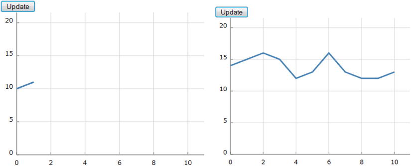
Figure 9-1. A real-time chart with a start button
Using PHP to Extract Data from a MySQL Table
Finally, the time has come to use data contained in a database, a scenario that is more likely to correspond with your daily needs. You choose MySQL as a database, and you use hypertext preprocessor (PHP) language to query the database and obtain the data in JavaScript Object Notation (JSON) format for it to be readable by D3. You will see that once a chart is built with D3, the transition to this stage is easy.
The following example is not intended to explain the use of PHP language or any other language, but to illustrate a typical and real case. The example shows how simple it is to interface all that you have learned with other programming languages. Often, languages such as Java and PHP provide an excellent interface for collecting and preparing data from their sources (a database, in this instance).
Starting with a TSV File
To understand more clearly the transition between what you already know and interfacing with PHP and databases, let us start with a case that should be familiar to you (see Listing 9-11). First, you write a tab-separated value (TSV) file with these series of data and save them as data_13.tsv.
Listing 9-11. data_13.tsv
day          income  expense
2012-02-12   52      40
2012-02-27   56      35
2012-03-02   31      45
2012-03-14   33      44
2012-03-30   44      54
2012-04-07   50      34
2012-04-18   65      36
2012-05-02   56      40
2012-05-19   41      56
2012-05-28   45      32
2012-06-03   54      44
2012-06-18   43      46
2012-06-29   39      52
![]() Note Notice that the values in a TSV file are tab separated, so when you write or copy Listing 9-11, remember to check that there is only a tab character between each value.
Note Notice that the values in a TSV file are tab separated, so when you write or copy Listing 9-11, remember to check that there is only a tab character between each value.
Actually, as hinted at, you have already seen these data, although in slightly different form; these are the same data in the data_03.tsv file (see Listing 3-60 in Chapter 3). You changed the column date to day and modified the format for dates. Now, you must add the JavaScript code in Listing 9-12, which will allow you to represent these data as a multiseries line chart. (This code is very similar to that used in the section “Difference Line Chart” in Chapter 3; see that section for explanations and details about the content of Listing 9-12.)
Listing 9-12. Ch9_02.html
<!DOCTYPE html>
<html>
<head>
<meta charset="utf-8">
<script src="http://d3js.org/d3.v3.js"></script>
<style>
body {
    font: 10px verdana;
}
.axis path,
.axis line {
    fill: none;
    stroke: #333;
}
.grid .tick {
  stroke: lightgrey;
  opacity: 0.7;
}
.grid path {
    stroke-width: 0;
}
.line {
    fill: none;
    stroke: darkgreen;
    stroke-width: 2.5px;
}
.line2 {
    fill: none;
    stroke: darkred;
    stroke-width: 2.5px;
}
</style>
</head>
<body>
<script type="text/javascript">

var margin = {top: 70, right: 20, bottom: 30, left: 50},
    w = 400 - margin.left - margin.right,
    h = 400 - margin.top - margin.bottom;

var parseDate = d3.time.format("%Y-%m-%d").parse;

var x = d3.time.scale().range([0, w]);
var y = d3.scale.linear().range([h, 0]);

var xAxis = d3.svg.axis()
    .scale(x)
    .orient("bottom")
    .ticks(5);

var yAxis = d3.svg.axis()
    .scale(y)
    .orient("left")
    .ticks(5);

var xGrid = d3.svg.axis()
    .scale(x)
    .orient("bottom")
    .ticks(5)
    .tickSize(-h, 0, 0)
    .tickFormat("");

var yGrid = d3.svg.axis()
    .scale(y)
    .orient("left")
    .ticks(5)
    .tickSize(-w, 0, 0)
    .tickFormat("");

var svg = d3.select("body").append("svg")
    .attr("width", w + margin.left + margin.right)
    .attr("height", h + margin.top + margin.bottom)
    .append("g")
    .attr("transform", "translate(" + margin.left + ", " + margin.top + ")");

var line = d3.svg.area()
    .interpolate("basis")
    .x(function(d) { return x(d.day); })
    .y(function(d) { return y(d["income"]); });

var line2 = d3.svg.area()
    .interpolate("basis")
    .x(function(d) { return x(d.day); })
    .y(function(d) { return y(d["expense"]); });

d3.tsv("data_13.tsv", function(error, data) {
    data.forEach(function(d) {
       d.day = parseDate(d.day);
       d.income = +d.income;
       d.expense = +d.expense;
    });

    x.domain(d3.extent(data, function(d) { return d.day; }));
    y.domain([
       d3.min(data, function(d) { return Math.min(d.income, d.expense); }),
       d3.max(data, function(d) { return Math.max(d.income, d.expense); })
  ]);

    svg.append("g")
       .attr("class", "x axis")
       .attr("transform", "translate(0, " + h + ")")
       .call(xAxis);

  svg.append("g")
    .attr("class", "y axis")
    .call(yAxis);

    svg.append("g")
       .attr("class", "grid")
       .attr("transform", "translate(0, " + h + ")")
       .call(xGrid);

    svg.append("g")
       .attr("class", "grid")
       .call(yGrid);

    svg.datum(data);

    svg.append("path")
       .attr("class", "line")
       .attr("d", line);

    svg.append("path")
       .attr("class", "line2")
       .attr("d", line2);
});

var labels = svg.append("g")
    .attr("class", "labels");

labels.append("text")
    .attr("transform", "translate(0, " + h + ")")
    .attr("x", (w-margin.right))
    .attr("dx", "-1.0em")
    .attr("dy", "2.0em")
    .text("[Months]");

labels.append("text")
    .attr("transform", "rotate(-90)")
    .attr("y", -40)
    .attr("dy", ".71em")
    .style("text-anchor", "end")
    .text("Millions ($)");

var title = svg.append("g")
    .attr("class", "title")

title.append("text")
    .attr("x", (w / 2))
    .attr("y", -30 )
    .attr("text-anchor", "middle")
    .style("font-size", "22px")
    .text("A Multiseries Line Chart");
</script>
</body>
</html>
With this code, you get the chart in Figure 9-2.
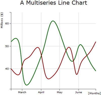
Figure 9-2. A multiseries chart reading data from a TSV file
Moving On to the Real Case
Now, let us move on to the real case, in which you will be dealing with tables in the database. For the data source, you choose a table called sales in a test database in MySQL.After you have created a table with this name, you can fill it with data executing an SQL sequence (see Listing 9-13).
Listing 9-13. sales.sql
insert into sales
values ('2012-02-12', 52, 40);
insert into sales
values ('2012-02-27', 56, 35);
insert into sales
values ('2012-03-02', 31, 45);
insert into sales
values ('2012-03-14', 33, 44);
insert into sales
values ('2012-03-30', 44, 54);
insert into sales
values ('2012-04-07', 50, 34);
insert into sales
values ('2012-04-18', 65, 36);
insert into sales
values ('2012-05-02', 56, 40);
insert into sales
values ('2012-05-19', 41, 56);
insert into sales
values ('2012-05-28', 45, 32);
insert into sales
values ('2012-06-03', 54, 44);
insert into sales
values ('2012-06-18', 43, 46);
insert into sales
values ('2012-06-29', 39, 52);
Preferably, you ought to write the PHP script in a separate file and save it as myPHP.php. The content of this file is shown in Listing 9-14.
Listing 9-14. myPHP.php
<?php
    $username = "dbuser";
    $password = "dbuser";
    $host = "localhost";
    $database = "test";

    $server = mysql_connect($host, $username, $password);
    $connection = mysql_select_db($database, $server);
    $myquery = "SELECT * FROM sales";
    $query = mysql_query($myquery);

    if ( ! $myquery ) {
       echo mysql_error();
       die;
    }

    $data = array();
    for ($x = 0; $x < mysql_num_rows($query); $x++) {
         $data[] = mysql_fetch_assoc($query);
    }
    echo json_encode($data);
    mysql_close($server);
?>
Generally, a PHP script is recognizable by its enclosure in special start and end processing instructions: <?php and ?>. This short but powerful and versatile snippet of code is generally used whenever we need to connect to a database. Let us go through it and look at what it does.
In this example, dbuser has been chosen as user, with dbuser as password, but these values will depend on the database you want to connect to. The same applies to the database and hostname values. Thus, in order to connect to a dabase, you must first define a set of identifying variables, as shown in Listing 9-15.
Listing 9-15. myPHP.php
$username = "homedbuser";
$password = "homedbuser";
$host = "localhost";
$database = "homedb";
Once you have defined them, PHP provides a set of already implemented functions, in which you have only to pass these variables as parameters to make a connection with a database. In this example, you need to call the mysql_connect() and myqsl_select_db() functions to create a connection with a database without defining anything else (see Listing 9-16).
Listing 9-16. myPHP.php
$server = mysql_connect($host, $username, $password);
$connection = mysql_select_db($database, $server);
Even for entering SQL queries, PHP proves to be a truly practical tool. Listing 9-17 is a very simple example of how to make an SQL query for retrieving data from the database. If you are not familiar with SQL language, a query is a declarative statement addressed to a particular database in order to obtain the desired data contained inside. You can easily recognize a query, as it consists of a SELECT statement followed by a FROM statement and almost always a WHERE statement at the end..
![]() Note If you have no experience in SQL language and want to do a bit of practicing without having to install the database and everything else, I suggest visiting this web page from the w3schools web site: www.w3schools.com/sql. In it, you’ll find complete documentation on the commands, with many examples and even the ability to query a database on evidence provided by the site by embedding an SQL test query (see the section “Try It Yourself”).
Note If you have no experience in SQL language and want to do a bit of practicing without having to install the database and everything else, I suggest visiting this web page from the w3schools web site: www.w3schools.com/sql. In it, you’ll find complete documentation on the commands, with many examples and even the ability to query a database on evidence provided by the site by embedding an SQL test query (see the section “Try It Yourself”).
In this simple example, the SELECT statement is followed by '*', which means that you want to receive the data in all the columns contained in the table specified in the FROM statement (sales, in this instance).
Listing 9-17. myPHP.php
$myquery = "SELECT * FROM sales";
$query = mysql_query($myquery);
Once you have made a query, you need to check if it was successful and handle the error if one occurs (see Listing 9-18).
Listing 9-18. myPHP.php
if ( ! $query ) {
    echo mysql_error();
    die;
}
If the query is successful, then you need to handle the returned data from the query. You place these values in an array you call $data, as illustrated in Listing 9-19. This part is very similar to the csv() and tsv() functions in D3, only instead of reading line by line from a file, it is reading them from a table retrieved from a database. The mysql_num_rows() function gives the number of rows in the table, similar to the length() function of JavaScript used in for() loops. The mysql_fetch_assoc() function assigns the data retrieved from the query to the data array, line by line.
Listing 9-19. myPHP.php
$data = array();
for ($x = 0; $x < mysql_num_rows($query); $x++) {
    $data[] = mysql_fetch_assoc($query);
}
echo json_encode($data);
The key to the script is the call to the PHP json_encode() method, which converts the data format into JSON and then, with echo, returns the data, which D3 will parse. Finally, you must close the connection to the server, as demonstrated in Listing 9-20.
Listing 9-20. myPHP.php
mysql_close($server);
Now, you come back to the JavaScript code, changing only one row (yes, only one!) (see Listing 9-21). You replace the tsv() function with the json() function, passing directly the PHP file as argument.
Listing 9-21. Ch9_02b.html
d3.json("myPHP.php", function(error, data) {
//d3.tsv("data_03.tsv", function(error, data) {
    data.forEach(function(d) {
       d.day = parseDate(d.day);
       d.income = +d.income;
       d.expense = +d.expense;
});
In the end, you get the same chart (see Figure 9-3).

Figure 9-3. A multiseries chart obtaining data directly from a database
Summary
This chapter concluded by considering two different cases. In the first example, you saw how to create a web page in which it is possible to represent data you are generating or acquiring in real time. In the second example, you learned how to use the D3 library to read the data contained in a database.
In the next chapter, I will cover a new topic: controls. I will describe the importance of introducing controls in a chart, understanding how you can change the chart property using controls. This affords the user the opportunity to select a property’s attributes in real time.