J. Chew1, H.M. Joshi2, S.G. Kazarian3, M. Millan-Agorio4, F.H. Tay5, and S. Venditti61Lecturer in Chemical Engineering, University of Bath, UK2Principal Heat Transfer Engineer, Shell, USA3Professor of Physical Chemistry, Imperial College London, UK4Reader in Chemical Engineering, Imperial College London, UK5Head of R&D, EliteTNS, Singapore6R&D Engineer, Resource Centre for Environmental Technologies, Luxembourg
Abstract
The analysis of the structure and chemistry of deposits formed by the crude oil fouling process is paramount in gaining an understanding of the underlying causes and mechanisms. Chapter 4 begins with a review of industrial practice and findings in this context and suggests recommended practice for the collection, preparation, and analysis of refinery samples. The second part of this chapter discusses more advanced techniques for the determination of the chemical structure and molecular weight of deposits and the third part of Chapter 4 introduces a novel technique (chemical imaging) by which the location of various chemical species in a surface layer can be established. The final part of Chapter 4 gives a description of a fluid dynamic gauging technique developed for measuring the thickness and strength of deposits in situ, in real time, and in a liquid environment.
Analytical characterization of crude oil deposits provides useful insights into understanding the underlying mechanisms leading to fouling, to determine its root cause and to find the sources of foulant precursors. Results of fouling deposit characterization can be used to establish the most appropriate method for preventing fouling or cleaning the fouled heat exchanger. For example, if the deposit is predominantly inorganic, coking mechanisms can be ignored and the focus can be shifted to find the source of the inorganic materials (e.g., desalter malfunction).
There is no single analytical technique that can provide a complete characterization of crude oils and crude oil deposits. Instead, their analysis must rely on a combination of several methods, each capable of providing partial information about the sample composition. This limitation in the scope of the characterization methods arises in part from the limitation of the analytical techniques themselves and in part from the complexity of the samples.
This chapter illustrates the use of characterization and measuring techniques of crude oil fouling deposits in refinery heat exchangers. Note that the same techniques can be applied to other fouling deposits such as those generated by experimental rigs (e.g., those described in Chapter 3), in other refining processes, or other industrial equipment.
Section 4.1 is concerned with the industrial practice and provides guidelines on deposit collection and sample preparation and illustrates how the lessons from deposit analysis can be used to effectively solve operating problems in the refinery. Section 4.2 shows the results of a detailed chemical structure and molecular weight characterization of refinery deposits. Section 4.3 presents results for the analysis of crude preheat train deposits using chemical imaging techniques. Finally, Section 4.4 is concerned with the measurement of thickness of fouling deposits, an important parameter when considering operations of heat exchangers.
4.1. Analysis of Field Fouling Deposits from Crude Heat Exchangers
H. M. Joshi
As discussed in Section 2.1, there are different mechanisms that lead to crude oil fouling in preheat trains (PHTs). Plant experience shows that the most common one is a combination of chemical reaction and corrosion fouling. In this mechanism, a mix of crude and inorganic particles is trapped in the roughness of the tube surface and generates deposits that degrade with time to a coke-like material according to the ageing mechanisms described in Section 2.3.5. The corrosion of the tube wall is believed to lead to the formation of an iron sulfide layer that further increases the roughness of the tube surface and consequently its ability to trap crude oil and other particles. The foulant material in this mechanism typically consists of a mixture of organics, salts, and FeS.
A second, less commonly observed, mechanism is that of deposition of precipitated asphaltenes on the tube wall and their eventual degradation to coke-like material. This typically happens when the crude or crude blend is incompatible (also called unstable) with respect to asphaltenes. The foulant material in this mechanism consists mostly of coke-like (organic) material.
A quantitative analysis of the deposit helps to identify which of the two mechanisms is dominant. If it is the more common fouling mechanism (i.e., with sulfide formation), the amount of different inorganic materials can point to the source of precursors, and the hydrogen and carbon quantities provide information about the temperature relationship of foulant formation. Moreover, regardless of the mechanism, a correct analysis can identify if an unexpected contaminant is responsible for the initiation of fouling.
When analyzing samples of crude oil deposits, to understand and correct operating problems, it is important to know whether fouling is dominated by organic or inorganic deposits, if it is a mix of the two, or if it is driven by a specific reaction mechanism generated, for example, by the use of chemical additives such as those added to prevent corrosion.
To perform an analysis that provides the most useful information, without expensive and time-consuming testing, three major steps are required:
1. Careful deposit collection
2. Correct sample preparation before testing
3. Appropriate sequence of analytical tests.
One such methodology is described by Brons et al. (2010).
This section proposes a recommended methodology to accurately quantify the deposit composition in real-life crude heat exchangers. This includes guidelines for appropriate sample collection, preparation, and analysis. Moreover, indications on practical interpretation of the analysis into actionable recommendations for the plant are provided.
4.1.1. Sample Collection
Sample collection is a relatively simple activity but a few guidelines must be followed to ensure an effective deposit analysis. Two key aspects during sample collection are to preserve the chemical integrity of the sample as much as possible, and to make a clear note of the location of the sample and take photographs of the fouled heat exchanger.
The recommended guidelines for sample collection are as follows:
• Shutdown procedure. Safety and environmental considerations require a minimum amount of cleaning, steaming, or flushing (sometimes referred to as decontamination) before a heat exchanger is opened. So that the chemical integrity of the deposit sample is preserved as much as possible, any additional cleaning should be avoided before sample collection. For example, washing with water will dissolve salts, which in some instances could be a large component of the foulant.
• Collection of the samples. If it visually appears that the deposits look different at different locations in the heat exchanger, collect multiple samples. Samples from different locations should be clearly marked as to exactly where they were taken, and should not be mixed. Moreover:
• Tube-side samples should be taken as far inside the tube as possible, and as close to the tube wall as possible. If there is widespread deposit on the tubesheet, or tube inlets are plugged, those deposits should be collected as separate samples.
• On the shell-side, if it appears that there are different levels and types of fouling in different areas of the exchanger, again collect separate samples. It is important to take at least one sample from the tube outside surface. This is critical for differentiating between a mechanism that is purely a deposition of particles carried in the stream and a mechanism that occurs due to either corrosion or coking at the tube surface. If the samples are collected only from the gap between tubes or the window areas it is possible that the mechanism at the tube surface will be missed at the analytical stage.
• Quantities. Fifty or more grams of foulant should be collected for each sample. If this is not possible, as much sample material as possible should be collected. As it will be explained later, a large amount of this collected material might be lost during sample preparation, thus it is important to have a sufficient quantity remaining to perform all the analyses required.
• Records. Keep accurate records of the exact location of the samples. Ideally photographs should be taken during this process to have a record of whether fouling is localized, how much is present in different parts of the exchanger, where the baffles are, etc.
• Storage. Store the samples in an airtight jar, to avoid the possibility of oxidation of its inorganic components.
4.1.2. Sample Preparation
Samples collected as per the above guidelines contain the process fluid (crude) which either is trapped within the deposit or is simply coating the samples. In addition, the deposit may be contaminated with flushing solutions or water from a steam-out (i.e., the process of circulating steam to remove contaminants). The trapped fluids or flushing solutions are not part of the foulant and need to be removed before the deposit is analyzed. This is a critical step because leftover process fluid or other contaminants will lead to mischaracterize the chemical makeup of the deposit, especially with respect to the quantification of the organic portion. The measured carbon and hydrogen content will be much higher than what is in the actual foulant (the deposit that creates the heat transfer resistance), leading to the possibly wrong conclusion that the fouling is dominated by organic mechanisms (i.e. asphaltene precipitation).
Solvents such as toluene or methylene chloride are used to dissolve and remove residual feeds and other liquids. An effective sample preparation procedure is described below.
• Add a sufficient quantity (e.g., 10:1) of the solvent in 10–15g of the collected deposit to dissolve trapped process fluid.
• Leave the mixture at room temperature for a few hours in an airtight jar.
• Filter the mixture and wash with additional solvent a few times until all the trapped fluid is removed—indicated by the filtrate being colorless.
• Dry the remaining deposit for several hours, preferably in a vacuum oven at an elevated temperature, 50°C or higher.
• Grind and mix the sample as much as possible to obtain a homogeneous powder. Since the interest is in the average composition of the deposit, this step is important to ensure that the final analyses are not conducted on a small and unrepresentative portion of the sample that happens to be rich in one component.
Most samples visually look the same when they are collected in the field. This is usually due to the trapped crude which gives the samples a black color and the appearance of a gooey mixture (often described by plant personnel as “shoe polish”). However, samples will look different when the above preparation is complete and a dry powdery deposit is obtained.
All further analyses detailed below should be conducted on this washed, dried, and homogenized sample. Depending on how much crude was trapped in this deposit when it was removed from the heat exchanger, this final sample might weigh substantially less (<40%) than the original one collected in the field.
4.1.3. Deposit Analysis Philosophy
The sample collection and preparation steps apply to any deposit for which a good quantification is needed for root cause determination or for developing a mitigation strategy. However, subsequent analyses of deposits from crude heat exchangers can be simplified, relative that described by Brons et al. (2010). This is mainly due to the fact that most of the time (about 90%) the fouling mechanism for crudes in operation is one of the two described at the beginning of the section (i.e., (1) chemical reaction/corrosion fouling or (2) precipitation of asphaltenes and their degradation to a coke-like material on the surface). To distinguish between these mechanisms, quantification of only a few elements is critical. This simplified set of tests will be referred to as Level 1 testing (L1). Depending on the results of L1 testing, the need for more specialized and detailed analysis can be established. In these cases (typically 10% of the times), Level 2 testing (L2) will be performed. Figure 4.1 shows a flow chart of the recommended test sequence.
Note that this strategy is aimed at identifying which of the two mechanisms is predominant and providing the refinery with suggestions for corrective actions. Even more detailed analyses (e.g., those described in Sections 4.2 and 4.3) are available to provide a deeper understanding of the fouling mechanisms themselves.
The next sections will describe the recommended analysis in Level 1 and Level 2 testing, and provide examples of analyses performed on deposits collected from oil refineries.
4.1.4. Level 1 Testing
4.1.4.1. Thermogravimetric Analysis
Thermogravimetric analysis (TGA) is a method for characterization of thermophysical properties of materials by probing into thermodegradation reactions at high temperatures. In a TGA test a small amount of sample (10mg) is placed in a platinum pan under an inert atmosphere inside a glass enclosure. The temperature inside the enclosure is increased from ambient to a maximum temperature (between 600 and 900°C), at a constant rate (e.g., 10°Cmin−1). As the sample is heated, different components of the deposit volatilize at different temperatures, providing information on deposit composition that can be linked to the possible causes of fouling. The response of the sample to heat is determined by accurately measuring the temperature and the decreasing mass inside the pan. Once the maximum temperature is reached, the inert atmosphere in the enclosure is replaced by air or oxygen and the temperature is held constant for a specific amount of time (e.g., 20min). This results in combustion of the remaining sample. After the combustion phase the experiment is terminated and what remains in the pan is called “ash.”
Figure 4.1Crude fouling deposit analysis test sequence.
TGA provides a significant amount of useful information in a fast (2–3h total time) and inexpensive way. For this reason, TGA should be the first test to be performed and it is the one recommended if only one test were to be performed. The main advantage of TGA is that it provides an estimate of the relative quantities of volatile and nonvolatile organic materials, and inorganic materials. However, TGA data do not identify what elements are present, and consequently it cannot be determined, for example, whether the inorganic material is a corrosion product (like FeS) or salts (like carbonates) or something else. Further analysis is needed for confirmation of elements and for quantification.
Another point of interest in TGA is that it allows determination of whether polymeric material such as gums might be involved in the formation of fouling precursors. Polymeric material tends to be emitted at temperatures <370°C. If a large drop in mass is found in this temperature range, this can be related to the presence of polymers in the sample. This is rare for crude deposit samples and will not be included in the cases studied here.
Two examples of tests on crude oil fouling deposits are presented below, with interpretations of the results. One is for a sample containing a high percentage of organic material (Sample A) and the other for a sample with a large content of inorganic material (Sample B). For samples with compositions in between, some interpolation of the interpretations will apply.
In these examples the key test parameters, such as the rate of temperature increase (10°Cmin−1), the time allowed for combustion (20min), and, particularity, the maximum temperature (800°C), have been selected on the basis of the author's own experience with crude deposit analysis. Different values can be used in practice.
Sample A has been collected from a heat exchanger toward the hot end of a crude PHT train. The TGA analysis for this sample is shown in Figure 4.2. The sample is heated from ambient temperature (about 30°C) to 800°C in ca.75min. During this heating period about 53% of the mass has volatilized; a further 25% weight loss occurred as a result of combustion when air was introduced at 800°C. The 53% loss of mass before the combustion step corresponds to easily volatilized material and does not need to be combusted. However, the entire 78% mass is organic foulant material. It is foulant formed as a result of the crude being subjected to the high tube wall surface temperatures, and is thermally degraded material that is insoluble in the solvent used to prepare the sample. This is usually referred to as coke or coke-like material. The 25% that combusted is hardened coke, presumably because it has been exposed for a longer time at the high temperature, so as to allow it to harden and become nonvolatile.
Figure 4.2Thermogravimetric analysis result for crude heat exchanger deposit for Sample A.
The large organic content of Sample A indicates that fouling may have occurred in this heat exchanger because of crude incompatibility. The 22% ash collected at the end of the test is inorganic material and further elemental or other analysis (on the prepared sample, not on the ash) is needed to know what, if any, elements or compounds are dominant.
Sample B is another sample from an atmospheric distillation unit preheat train but it exhibits a completely different behavior when characterized with TGA. Figure 4.3 shows how Sample B contains about 10% of organic material and 90% inorganic material (ash). Inorganic materials flow with crude streams in the form of corrosion products (usually iron sulfide) and salts (typically sodium and calcium salts—carbonates, chlorides, sulfates). For this sample, further elemental analysis is needed to determine which inorganic materials are prevalent. Identifying the exact inorganic species present is key to determining the correct fouling mitigation strategy that will eliminate those components or prevent them from depositing on the tube wall.
Figure 4.3Thermogravimetric analysis result for crude heat exchanger deposit for Sample B.
4.1.4.2. Elemental Analysis
Elemental analysis for typical crude deposits involves three types of tests to quantify:
• Carbon, hydrogen, and nitrogen (CHN) content.
• Sulfur content.
• Presence of metals and other inorganic elements.
The determination of which of these tests is necessary should usually be done on the basis of the TGA results. For example, because of the large organic content, for Sample A (Figure 4.2), the CHN test will be sufficient to confirm the asphaltene precipitation mechanism, whereas for Sample B (Figure 4.3), only sulfur and metals need to be measured. All three tests should otherwise be conducted for deposits showing compositions in between, because in these cases both organic and inorganic fouling precursors play a role.
4.1.4.2.1. Carbon, Hydrogen, and Nitrogen Testing
CHN testing focuses on quantifying C, H, and N content in a particular sample. A good method for this type of analysis is provided by the ASTM standard D5373 (ASTM, 2014a). Results are reported as weight percent of the elements in the deposit. There are two useful ways of using data collected from this test. First, CHN tests can be used as a confirmation of the TGA results. The sum of the weight percentages measured with CHN tests should roughly be equal to the organic content inferred from the TGA. For example, in CHN tests for Sample A (Fig. 4.2), the results show C=70%, H=5.5%, and N=1%, for a total of ca. 77%, consistent with the ca. 22% ash remaining from TGA.
The other useful information is the atomic H/C ratio calculated as:
H/C=12×weight%Hweight%C
For Sample A, the H/C=5.5/77×12=0.86. As the deposit thermally degrades (dehydrogenates) in the operating heat exchanger, over time its H/C ratio decreases. Moreover, the higher the temperature to which the deposit is exposed (the tube wall surface temperature), the faster the rate of degradation. The H/C ratio from a typical deposit is a function of the temperature at which this coke-like material was formed, over a reasonably long time frame, which, for crude heat exchangers, is typically over 6months. In crude preheat train exchangers the wall surface temperatures in the hotter part of the train are between 200°C and 330°C, and the corresponding expected H/C ratio range is 0.80–0.95.1 The ratio measured in Sample A falls in this range, which further confirms the results of TGA. If the H/C ratio is higher than 0.95, the deposit has degraded less, which implies that the residence time has not been long enough for the deposit to fully age to a coke-like material. More interesting is the case where this ratio is lower than the above range, ca. 0.70 or lower. In this case, the deposit degraded at a temperature higher than a typical crude preheat. One possible conclusion then is that the foulant was not formed in the heat exchanger but came in with the crude as already formed coke and deposited in the heat exchanger.
4.1.4.2.2. Sulfur Testing
In fouling deposits from crude heat exchangers, sulfur is almost always present, and usually in the form of iron sulfide (FeS). Sometimes it is present in the form of sulfates and sometimes as elemental sulfur with the organic material. The iron sulfide may also be pyrrhotite, a form with a variable iron content: Fe(1–x)S (x=0–0.2).
A good method for sulfur quantification is the ASTM standard D4239 (ASTM, 2014b). This test gives important information regarding the association of the elements. If the iron and sulfur are in a molar ratio in the range 1 to 0.8 (i.e., with x in the range 0–0.2), it is reasonable to conclude that most of the iron and sulfur are present as iron sulfide (Fe(1–x)S). If the total of Fe and S is a high percentage, e.g., >50%, then at least one of the dominant fouling mechanisms is corrosion based. This includes FeS carried in with the crude or severe sulfur corrosion of the tube surface itself, which contributes to the fouling. High velocities will minimize the deposition of carried-in FeS.
If there is more sulfur in the sample than indicated by the Fe(1–x)S formula, then the excess will be present as metal sulfates or organic sulfur.
4.1.4.2.3. Testing for Other Chemical Elements
Testing for elements other than C, H, N, and S becomes important when the amount of TGA ash is not insignificant, i.e., >30%. The common elements found in crude fouling deposits are:
• Nonmetals: Chlorine (Cl), silicon (Si), and phosphorus (P).
Among these elements, iron is usually in the largest quantity followed by Cr, Na, and Ca. If sodium is present as a chloride, a stoichiometrically consistent amount of chlorine will usually be detected. The other metals could be in the form of oxides, chlorides, sulfates, or carbonates.
The importance of this elemental testing is twofold: to quantify the amount of iron, as explained in the earlier section on sulfur testing; and to identify if any single element could be responsible for the fouling mechanism, particularly if it is present in large quantities. For example, a large amount of silicon might point to a mechanism where silica is carried in with the incoming crude and deposits due to low velocities. In this case, one possible method of fouling mitigation will be to eliminate the source of the silica.
Similarly, if an unexpected element is detected in a significant amount (>5%), a possible explanation of its presence and a possible cause for fouling is the addition of chemicals either in the crude processing unit itself or upstream all the way to the production facility.
A reliable method for quantifying the elements important to crude fouling deposit analyses is inductively coupled plasma optical emission spectrometry (ICP-OES). Several commercial analytical laboratories provide this test, and sometimes it can be ordered for specific elements only.
4.1.4.2.4. Oxygen Testing and Calculation
A large amount of oxygen (up to ca. 20%) is sometimes found in organic fouling deposits originating from polymers, where oxygen catalyzes the reactions, or where it is a part of the process chemistry. However, in crude oil fouling deposits, this is an exception and only occasionally large quantities of oxides, e.g., silica, will result in a high oxygen content in the deposit.
Oxygen quantification is typically not needed as the amount of oxygen can usually be quantified using the measured silicon. This typically allows bringing the mass balance to a satisfactory closure. However, since some of the metals could be present as oxides, sulfates, or carbonates, sometimes it is necessary to calculate the amount of oxygen that may be present. This helps to close the mass balance of the deposit components, as will be explained in the following section. If oxygen measurement becomes necessary because the mass balance is not closed, a reliable method of quantification that can be used is neutron activation analysis (NAA).
4.1.4.3. Mass Balance
When all the testing is finished, an important step for verifying the quality of the results is to check the mass balance by adding the measured weight percentages of each measured elements. Experience shows that for most crude-related deposits the percentages of the CHN, S, and other metals only rarely add up to 100%. Typically mass balances add up to about 85–95%. Some of this inaccuracy is due to the nonhomogeneity of the samples (despite the care taken to grind and homogenize in the sample preparation step), although some might be due to the accuracy of the measurements.
One step to bring the mass balance closer to 100% is to guess whether oxygen might be associated with certain elements (Si and Al are typical candidates), and calculate how much is needed to have them present as oxides. For example, for silicon to be present as SiO2 requires the masses of silicon and oxygen to be in the ratio of 28:32. If there is 10% Si in the deposit it is reasonable to expect 11–12% oxygen (which was not part of the measurements).
For the purpose of characterizing a field deposit, an analysis resulting with a mass balance of 90% or better is considered adequate to identify the root cause of fouling and to determine appropriate mitigation or cleaning methods.
To illustrate the concepts above, the analyses of two samples, reported in Table 4.1, are considered. Measured weight percentages for the first sample, Sample C, show an acceptable closure of the mass balance. The second analysis, for Sample D, shows the need to calculate the percentage of oxygen to close the mass balance. In this case it is assumed that silicon is present as SiO2. Based on experience it can be determined that Si and Al in Sample C are likely to be oxides, and some of the sulfur might be in the form of sulfates. This can be confirmed with Level 2 analysis, and in particular with X-ray diffraction (XRD) and microscopy. If oxygen is calculated with those assumptions the final mass balance will be close to 90% and judged satisfactory.
In cases where it is impossible to close the mass balance to a reasonable accuracy, two possibilities exist. Either an error was made in one of the tests—in which case a repeat is necessary—or there is a missing element for which no testing was done. Experience shows that if a reputable laboratory is used to conduct the testing, it is more likely that an element has been missed. For example, when an ICP-OES test is ordered, the laboratory might provide a standard set of results, or some charge for the test on a per element basis and may not have provided the missing element. Typically, an understanding of the operation of the process unit helps to identify why an unexpected chemical is present in the deposit. This includes, for example, whether external additives are injected in the process (e.g., for corrosion control), if temporary streams (such as slops) are being mixed with the crude feed. However, in some cases, this may not be enough to identify a specific fouling mechanism (with related mitigation action) and additional, more detailed testing should be conducted.
Table 4.1
Example of two mass balances for different samples. For Sample C, the sum of the measured percentages provide a satisfactory closure of the mass balance. For Sample D oxygen calculations are needed to close the mass balance satisfactorily.
Element
Sample C, wt%
Sample D, wt%
C
35.80
23.00
H
4.61
1.70
N
0.50
0.20
S
16.62
13.00
Cl
2.16
–
Si
0.89
17.00
Fe
23.90
22.00
Na
1.93
0.45
Al
0.46
–
Ca
1.66
–
Zn
1.44
–
V
–
0.35
Total
89.97
77.70
O calculated
–
19.43
Overall
89.97
97.13
4.1.5. Level 2 Tests
At the completion of Level 1 tests, the results of the analysis on a particular sample include the TGA profile and the weight percentage of various elements. For deposits from crude heat exchangers this information is sufficient in 90–95% of the cases to come to usable conclusions and provide guidance to the refinery.
For a few cases, more detailed, Level 2 testing might be required. The intent of Level 2 testing is to gain a deeper understanding of the fouling mechanism, the processes of deposition and coke formation, the exact chemical nature of the compounds, or to identify precursors that otherwise may not be found. Although these types of testing are rarely conducted in industrial practice, they provide key information in nonstandard cases.
4.1.5.1. Carbon as Carbonate Analysis
If a large amount of carbonate is present in a deposit, meaning a portion of the measured carbon is inorganic, the mass balance will be difficult to match because the measured carbon is normally assumed to be organic. In addition, the H/C ratio might look inconsistent with what is expected in a particular deposit. In such a case, a test to quantify the amount of carbon present as carbonate will be useful. One example of such a test is the ASTM standard D6316 (ASTM, 2009).
4.1.5.2. Sulfur Forms Determinations
Total sulfur quantification was described in Section 4.1.4.2. Further analysis of sulfur to identify sulfates or organic sulfur is usually unnecessary but it is a good tool to have when the amount of measured sulfur cannot be explained by association with iron alone.
The ASTM standard D2492 (ASTM, 2012) is a good method for the determination of the percentages of pyritic sulfur and sulfates. Subtracting these from the total sulfur determined from L1 analysis gives the amount of organic sulfur.
4.1.5.3. Neutron Activation Analysis
Neutron activation analysis is a reliable method for measuring oxygen. However, as noted previously under the discussion for oxygen, this test is rarely needed for crude deposits.
4.1.5.4. X-Ray Diffraction
XRD is used to identify specific crystalline compounds or to identify specific phases of crystalline substances such as the type of iron sulfide present in the deposit. This is useful when such specific knowledge is needed, but not necessary for the typical fouling mechanisms of crude oils in heat exchangers.
4.1.5.5. Optical Microscopy
Cross-polarized light optical microscopy is particularly useful in identifying the nature of the coke in the fouling deposit. An expert eye can interpret the results and infer the coke formation mechanism (e.g. whether asphaltenes could have been the precursors), determine the size of inorganic particle in the deposit and obtain other similar information. Figure 4.4 shows an example where inorganic particles (round catalyst fines) serve as nucleation sites for coke growth, and the optical microscopy image clearly reveals this.
Figure 4.4Example of optical microscopy.
4.1.5.6. Scanning Electron Microscopy
Scanning electron microscopy (SEM) is another advanced technique that can help to obtain a deeper understanding of the deposit composition as well as the fouling mechanism. For crude fouling deposits, the two most useful features provided by an SEM analysis are element mapping and a deposit profile.
Element mapping shows the association of one or more elements, to confirm the form in which they exist. For example, Figure 4.5 shows SME scans of a deposit where particles are identified with two different elements (Si on the left and O on the right). This confirms that silicon exists as an oxide.
Figure 4.5Example of scanning electron microscope element map.
If the fouling surface is available for microscopy, e.g., a fouled tube that was removed from the heat exchanger and cross-sectioned, it can be used to study the laydown pattern of the deposit. For example, SEM might show a layer of corrosion (FeS) closest to the surface, and then a layer of salts plus coke-like material.
4.1.6. Guide to the Interpretation of Results
Examples of interpretation of Level 1 analysis for two samples, both collected in crude preheat trains, are shown below. Sample E is very typical of crude preheat trains, in the heat exchangers downstream of the desalter. Sample F is for a specific case of crude oil incompatibility, and will be seen in the hottest part of the crude preheat. Results of TGA and elemental analysis for the two samples are summarized in Table 4.2.
From the TGA test for Sample E it can be seen that about 22% out of the 51% organic portion of the deposit is relatively hardened coke. This is the portion that combusts after air is added during the TGA test. This implies an active, temperature-related coking mechanism occurring in the exchanger. However, given the large inorganic component (45–50%) in the deposit, it can be concluded that this is not the dominant mechanism. From the elemental analysis, it can be seen that the total amount of organic material is ca. 51% (C, H, N, and perhaps some S). This is consistent with 46% ash from TGA and implies that the fouling is roughly an even mixture of coke-like material and inorganic deposits.
Table 4.2
Elemental analysis and TGA summary for Sample E and Sample F.
Element
Sample E wt%
Sample F wt%
C
46.20
77.20
H
3.30
5.00
N
1.00
1.00
S
9.10
2.80
Si
3.10
3.50
Cl
6.90
–
Fe
4.50
4.50
Ca
2.80
–
Na
3.30
–
Al
1.50
–
Mg
0.60
–
Ni
0.20
–
V
0.40
–
Total
82.90
94.00
O calculated
13.06
4.00
Overall
95.96
98.00
TGA
–
–
Volatilized
32.0
50.0
Combusted at 800°C
22.0
46.0
Ash
46.0
4.0
The inorganic part of the deposit is dominated by various salts. Since there is not sufficient iron for all the sulfur to be in the FeS form, it is assumed that some of the sulfur was present as sulfate. This is not uncommon in crude deposits, although it is also common to see the inorganic part dominated by iron sulfide. In this example iron sulfide is about 7% of the deposit.
In terms of the quality of the analysis, a close look at the overall mass balance indicated that it is necessary to calculate the oxygen content. In fact, the measured weight percentages added to ca. 83% and, assuming as per above that a large portion is sulfates, the oxygen calculations bring the mass balance to ca. 96%. As noted before, this is satisfactory for practical purposes and also eliminates any doubts that any element has been missed from the tests. If necessary, a sulfur forms test can be used for further confirmation.
The H/C ratio calculated from the HCN test is 0.86, which is consistent with the range expected in such samples (see Section 4.1.4.2 on CHN testing) and confirms that the organic material was formed in the heat exchanger.
From all the observations above, it can be concluded that the overall fouling mechanism for Sample E is a combination of inorganic particle deposition and coking of crude trapped at the surface in these deposits. Experience has shown that preventing deposition, by using high velocities (or shear stress), is the most cost-effective way of dealing with this type of fouling. It might be worth investigating whether the amount of salts can be reduced at their source; however, deposition will still occur at low velocities.
In the case of Sample F, TGA alone provides enough indication to determine the fouling mechanism with a high level of confidence even before conducting elemental analysis. In fact, the large organic (85–90%) material detected via TGA strongly suggests that the formation of the deposits is dominated by incompatibility between the crude oils mixed to form the inlet stream to the heat exchanger. The crude flowing through this heat exchanger has precipitated asphaltenes that agglomerate into large particles and deposit on the tube wall, where they eventually thermally degrade to coke-like material. A test for asphaltene compatibility can be performed to verify if this is the case. Most major oil companies, and several others that provide chemicals to them, have their own, proprietary, tests for asphaltene compatibility (also called asphaltene stability).
Although TGA would have sufficed to identify the fouling mechanism, the elemental analysis provides some more insights on the conditions under which the deposits were formed. The H/C ratio of 0.77 is slightly lower than the values expected in crude heat exchangers. This could be explained by two reasons: high surface temperature in the heat exchanger and/or a longer than usual residence time at the high temperatures.
Experience in dealing with this type of fouling indicates that the most effective way of reducing it is by controlling crude incompatibility, and by eliminating the precursors—precipitated asphaltenes. High velocities have been found not to help as much as they do when inorganic deposition plays a large role in fouling.
4.1.7. Conclusions—Use of Deposit Analysis Results
The previous sections have shown how characterization techniques can be used to postulate a fouling mechanism associated with a specific sample and how to use the results to guide fouling mitigation strategies in oil refineries. These have been discussed in various parts of this chapter—increase velocity, control crude incompatibility, minimize (upstream and in the heat exchanger tubes), remove dominant precursors at their source, and eliminate or control additives that may produce chemicals that promote fouling. Here the typical situations encountered with crude preheat heat exchanger deposits are summarized.
• If the sample composition is dominated by inorganic materials (i.e., corrosion products or salts make up at least 70% of the deposit), the likely fouling mechanism is particulate deposition due to low velocity (or shear stress). In this case, it is commonly believed that increased salt removal in a normally operating desalter has a beneficial impact on heat exchanger fouling. However, it is not proven in practice that this is true and the most effective remedy is likely to be an increase in fluid velocity or shear stress. Other means, e.g., tube inserts, which have the effect of increased shear stress have also proven to be effective in some cases. No economically viable methods (e.g., filtering) are currently known or practiced to mitigate this problem by removal of inorganic particles (which are typically smaller than 30μm in diameter thus difficult to capture).
• If iron sulfide is dominant in the deposit (>60%), the fouling mechanism is most likely corrosion based and it might be possible to prevent upstream corrosion and minimize its flow in to the heat exchangers (e.g., by changing metallurgy). However, this may not always be economically feasible as there is a large amount of equipment, piping, etc., upstream that contributes to the creation of these particles.
• If an unexpected element is detected in a relatively significant amount (i.e., more than a few percent for a species that is not expected at all), its presence can often be traced back to a chemical added upstream for purposes such as corrosion control or flow enhancement. Unfortunately, from an operational point of view, it may or may not be possible to control the usage and dosage of these chemicals and their effects.
• A deposit dominant in organic material (>70%) points to an asphaltene precipitation mechanism and to an incompatibility problem with the crude. This should be confirmed by an analysis of the crude. The effective way to deal with this fouling is by making the crudes compatible, but it depends on the economics of buying and blending different crudes, and being able to process them at the given refinery.
• The H/C ratio is significant in determining the nature of the coking process. A ratio >0.95 indicates organic material that is not yet fully degraded and can perhaps be washed away by a solvent. A ratio <0.8 indicates hardened material with long exposure to a hot surface, and a ratio <0.7 indicates exposure temperatures that are higher than those encountered in a crude heat exchanger. The last case is unlikely to be observed in a crude preheat train, and indicates that the organic material was formed elsewhere and not in the heat exchanger.
• If chemical cleaning—circulation of a solvent material—is being considered, the deposit composition will help to determine which solvent will be most suitable. For example, if water-soluble salts are dominant, a steam-out might provide a high degree of cleaning. Or, if the organic portion is dominant with H/C > 0.95, an aromatic solvent might be effective in dislodging the unconverted, partially soluble, material. Note that typical coke-like material (H/C < 0.9) and corrosion products are not soluble in the chemical cleaning agents that are currently in use.
4.2. Chemical Structure and Molecular Weight Characterization
M. Millan, S. Venditti
The previous section of this chapter has presented some recommended guidelines for quantitative analysis of heat exchanger deposits in refinery PHTs. This was aimed at identifying the dominant mechanism that leads to fouling and suggesting practical actions to remediate it. This section, based on work originally presented to the 8th Heat Exchanger Fouling and Cleaning Conference in Schladming, Austria (Venditti, 2009b), focuses on developing a more fundamental understanding of the nature of deposits and underlying fouling mechanisms. The development of a combination of techniques used for the characterization of heat exchanger deposits is presented using a case study on the analysis of four refinery samples. It is shown how several methods for the analysis of liquids and solids can be combined to gain a useful insight into the nature of deposits.
The analytical work combined liquid phase analysis of the soluble fractions of the deposits with analysis of the solid samples. For the liquid phase analysis, size-exclusion chromatography (SEC) and synchronous UV–fluorescence spectroscopy (UV-F) were used. For the solid samples, proximate analysis was carried out in a thermogravimetric analyzer and attenuated total reflection-Fourier transform infrared spectroscopy (ATR-FTIR) was used to examine the functional groups of the deposits and to calculate aromaticity indices. Also for the solid samples, scanning electron microscopy coupled to energy dispersive X-ray spectroscopy (SEM-EDX) and XRD have been used to obtain a better understanding of inorganic components in the deposits, which proved to be high in some cases. Despite the limitations of each technique, the results from this combined approach suggest its suitability for the study of crude oil deposits and complex carbonaceous materials.
The main features, advantages, and disadvantages of the analytical techniques whose use is described in the literature on fouling studies are summarized in Table A1 in the Appendix. Some of these techniques (i.e., TGA, elemental analysis (EA), XRD, optical microscopy, and SEM) have already been introduced in Section 4.1; thus this section will only provide, when appropriate, a brief description of SEC, UV-F, and ATR-FTIR.
4.2.1. Methodology
Table 4.3 lists the four heat exchanger deposits analyzed in this work. The origin of the samples is confidential. All samples originate from tube-side locations with exception of the sample DA (shell-side) and were collected by oil refinery operators, following standard shutdown protocols.
Initially, samples of deposits received from the refinery were extracted by a series of solvents, including chloroform, 1-methyl-2-pyrrolidinone (NMP), and toluene, to determine their solubility properties. The extracts were examined by SEC and UV-F, two techniques that have been developed in previous work for the characterization of several heavy hydrocarbon samples, including heavy oil fractions (Álvarez, 2008; Berrueco, 2008; Dabai, 2010; Karaca, 2004).
Table 4.3
Deposit samples used in this study ∗VGO (virgin gas oil) is a mixture of coker mid-distillate, light cycle oil, and vacuum gas oil.
Sample name
Unit
Exchanger side
Temperature range (°C)
Feed processed
PHTD
Atmospheric distillation preheat train
Tube
158–166
Desalted oil
KPHTD
Kero preheat train
Tube
240–260
Kerosene
DA
Desulfurizer train
Shell
Up to 315
VGO∗
DB
Residue processing
Tube
Up to 370
Oil residue
SEC is a liquid chromatography technique where a sample in solution is injected into a packed column containing a porous stationary phase. The solvent must be strong enough to avoid any interactions between the sample and the column packing, such that the separation takes place purely by molecular size. Small molecules are able to enter the pores and therefore they take a longer path than larger molecules. The latter are excluded from the column pores, eluting at shorter times.
UV-F involves the excitation of molecules in a dilute solution by UV radiation. In molecules presenting fluorescence the electrons return to the ground state, emitting light at a longer wavelength than that exciting the molecule. UV-F spectra can be recorded in three modes, emission, excitation, and synchronous. In emission spectra, excitation is carried out at a single wavelength and the emitted light is recorded in a range of frequencies. Excitation spectra involve excitation over a range of wavelengths and the fluorescence intensity is observed at a single wavelength. In synchronous spectra, both excitation and emission are varied simultaneously, but a constant wavelength difference between them is used. These fluorescence emission spectra reveal information about the abundance and types of functional groups present in fluorescent organic molecules. Of particular importance to the analysis of asphaltenes is the effect of polynuclear aromatic groups on the UV-F spectra. As the size of a fused aromatic ring increases, there is a shift in the fluorescence spectrum toward longer wavelengths, while the fluorescence intensity decreases.
The data collected with SEC and UV-F were combined with analysis of the insoluble material and samples of the whole deposit. The next section describes the characterization of the soluble fraction of the deposits and Section 4.2.3 presents the characterization of the whole deposits and their insoluble fractions.
4.2.2. Analysis of the Soluble Fraction of the Deposits
The first step in the characterization procedure was to test the solubility of the deposits in some common solvents. The results for the four deposits are listed in Table 4.4. DA and DB were less soluble in the solvents used, including toluene, compared to PHTD and KPHTD. This appears to match their exposure to higher temperatures, which contributed to the formation of a coke-like material.
The fractions of the samples soluble in NMP/CHCl3 6:1 ratio (vol/vol), the solvent mixture used as eluent in SEC, were analyzed by SEC and UV-F. Figure 4.6 presents the SEC chromatogram of the soluble fraction of the deposits. SEC chromatograms of heavy oil fractions and other heavy hydrocarbon samples typically show two peaks. At short elution times (corresponding to larger molecular sizes), between 10 and 13 min, a peak excluded from the column porosity appears. This represents material that due to its large molecular size cannot enter the column pores and therefore elutes in the space between solid phase particles, therefore having shorter paths and elution times. It has been shown in previous work that existing elution time calibrations (based principally on the use of polystyrene standards) overestimate the molecular masses of material eluting in the excluded range. This overestimation was linked to changes in conformation from relatively planar to rigid three-dimensional forms as in fullerenes (Karaca, 2004). The second peak corresponds to material retained by the column eluting at longer elution times. Calibrations have been proven to suitably describe material in the retained region of the chromatogram. The calibration for the column used in this work has been described by Berrueco (2008).
Table 4.4
Solubility of the deposits used in this study (see Table 4.3 for sources) PHTD are deposits from the atmospheric distillation preheat train, KPHTD are from the kero preheat train, DA are from the desulfurizer train, and DB are from residue processing
Solvent
Solubility (% of the Deposit)
PHTD
KPHTD
DA
DB
CHCl3
45
80
61
58
NMP
35
38
37
32
NMP:CHCl3
39
42
39
34
Toluene
43
46
33
34
Figure 4.6Size-exclusion chromatograms of the NMP:CHCl3 (6:1 vol/vol)-soluble fraction of heat exchanger deposits obtained in a mixed-D, size-exclusion chromatography column.
Clear differences were observed between the samples recovered from the four deposits. The retained peak was observed to shift to longer elution times (smaller molecular weights) from KPHTD to DA. This shows the presence of larger molecules in KPHTD compared to DA. The DB chromatogram shows a bimodal retained peak at intermediate values with a maximum intensity for the second peak around 23min. In terms of distribution, PHTD and KPHTD chromatograms showed the presence of larger molecules in comparison with DB, whereas DA consisted of predominantly light material, likely to have been occluded in the deposit without much alteration.
Intensity-normalized synchronous UV–fluorescence spectra of the deposits are presented in Figure 4.7. UV-F spectra show a shift toward longer wavelengths as the size of the polycyclic aromatic groups increases (Morgan, 2005). The spectra in Figure 4.7 show that DA contains the smaller aromatic chromophores of the four deposits and this can be related to the SEC results that showed that its molecular weight distribution was shifted to low values. The spectra display a shift toward longer wavelengths, from KPHTD to DB and to PHTD, suggesting the largest aromatic cores are in the PHTD sample.
4.2.3. Analysis of the Insoluble Fractions and the Whole Deposits
Heat exchanger deposits and their toluene-insoluble fractions were analyzed by TGA. TGA allowed the estimation of volatiles, ash content, and fixed carbon in the deposits and their fractions. The results are summarized in Table 4.5. All deposits showed a certain amount of light material that was volatile under the TGA conditions at temperatures up to 370°C. This was particularly high for DA (27%), which correlates well with the observations made by SEC and UV-F on the soluble fraction. PHTD and KPHTD, on the other hand, presented relatively high ash contents. It is clear that toluene solvent extraction took away most of the light volatiles and therefore the toluene-insoluble fractions showed a marked increase in the fixed carbon.
Figure 4.7Synchronous UV-F spectra of the NMP: CHCl3 (6:1 vol/vol)-soluble fraction of heat exchanger deposits.
Table 4.5
Proximate analysis of the deposits (PHTD, KPHTD, DA, and DB) and their toluene-insoluble fractions (PHTD-TI, KPHTD-TI, DA-TI, and DB-TI) carried out by TGA
Sample
Volatile loss by 370°C (%)
Total volatiles by 900°C (%)
Fixed carbon (%)
Ash (%)
PHTD
16.8
46.8
18.0
35.2
KPHTD
7.4
50.3
24.1
25.6
DA
27.0
61.1
33.0
5.9
DB
14.0
40.7
47.9
11.4
PHTD-TI
1.8
29.8
13.8
56.4
KPHTD-TI
2.7
18.9
39.9
41.2
DA-TI
1.0
39.9
57.0
3.1
DB-TI
4.0
21.7
63.3
15.0
The high ash content observed in KPHTD and PHTD triggered further analysis to identify the inorganic foulants present by XRD (Table 4.6) and SEM-EDX (Table 4.7). XRD is useful for identifying crystalline phases of inorganic components such as iron sulfide present in corrosion scale. As the toluene-insoluble fraction is regarded to be the main foulant component of the deposit, only those fractions were analyzed. High levels of iron and sulfur are present in all of the samples, especially in PHTD-TI and KPHTD-TI. The high ash, iron, and sulfur contents may indicate corrosion fouling as the main issue for PHTD and KPHTD.
Table 4.6
Inorganic species present in the ash of the deposits measured by X-ray diffraction (XRD). Analyses were carried out in the toluene-insoluble fraction of the deposits
Inorganics present by XRD
PHTD-TI
KPHTD-TI
DA-TI
DB-TI
FeS
Yes
Yes
Yes
Yes
NaCl
Yes
Yes
Yes
No
SiO2
No
No
No
Yes
BaSO4
No
No
No
Yes
CaSO4
No
No
No
Yes
FePO4
Yes
No
No
No
VS
No
No
No
Yes
MgAlSiO
No
Yes
No
No
AlSiO
No
Yes
No
No
ZnS
No
Yes
No
No
CaCO3
Yes
No
No
No
Table 4.7
Major inorganic elements present in the ash of the deposits measured by energy dispersive X-ray. Analyses were carried out on the toluene-insoluble fraction of the deposits
Inorganics present by XRD
PHTD-TI (wt%)
KPHTD-TI (wt%)
DA-TI (wt%)
DB-TI (wt%)
Na
3.8
2.7
0.1
0.2
Mg
0.3
1.3
–
0.1
Al
0.7
0.5
0.3
1.7
Si
1.5
7.2
0.2
1
K
0.2
–
–
–
P
0.2
–
0.1
0.5
Ca
2.2
1.7
0.2
1.1
V
–
–
–
0.8
Ba
0.9
–
–
1
Fe
10.4
8.8
5.3
4.9
Ni
–
–
0.2
0.7
Zn
1
1.4
–
–
XRD, X-ray diffraction.
For KPHTD-TI and PHTD-TI, the presence of salts was relevant. High levels of sodium were observed by SEM-EDX, with the presence of sodium chloride confirmed by XRD analysis. This result was somewhat unexpected considering that the feed processed in the PHTD unit was desalted crude. The deposition therefore appears related to incomplete desalting. Analysis of the KPHTD-TI sample also suggested the presence of magnesium silicate; possible sources are the reservoir itself or organic acid salts added during the production process.
The low ash content observed in the analysis of DA and DB suggests that they were mainly related to thermal decomposition due to the high operating temperature. In both cases, corrosion fouling was also observed. Sulfates and sulfides were detected, especially in DB-TI. The presence of Ni and V in DB also suggests a more asphaltenic nature. The DA ash content was found to be lower than that in DB. Originated from a vacuum gas oil feed, DA showed a lighter nature, which would explain the small differences between values for the DA sample and its toluene-insoluble fraction.
Figure 4.8 presents the ATR-FTIR spectra of the set of heat exchanger deposits. In ATR-FTIR, spectra are generated by interaction between the sample and an infrared beam internally reflected in a crystal. The IR beam propagates a few micrometers into the analyte in an evanescent wave and interacts with molecular vibrations in the sample. Each functional group in the sample's compounds has characteristic vibrational modes with frequencies corresponding to a certain energy and wavelength of the incident light. By this technique it is therefore possible to extract information on the functional groups present in the sample.
In this study, the ATR-FTIR spectra showed no bands in the 3900 to 3100 cm−1 region, indicating low concentrations of OH or NH groups. The region 3000–2800 cm−1, related to the aromaticity of the samples, presented high intensity peaks.
In the 1750–1600cm−1 region, all samples showed a peak about 1700 cm−1 corresponding to carboxylic acids with low intensity. The 1600cm−1 band is known as the coke band and was observed to shift to lower wavelengths in deposits aged for longer, in agreement with observations from the literature (Fan, 2006). These results showed the typical condensed polyaromatic structure of the aged deposits.
The band assignment in the 1300–1500cm−1 region corresponds to CH3 and CH2 alkyl chains bending mode. More intense signal in this region was observed in the cases of PHTD and KPHTD.
Figure 4.8Attenuated total reflectance infrared spectroscopy (ATR-FTIR) of heat exchanger deposits.
The band at 1100–950cm−1 is assigned to ethers, alcohols, and sulfoxides. The presence of C=S (1026cm−1) was observed in all four samples. However, the signal in this band is more evident for the DB and KPHTD samples. This result can be linked to corrosion due to sulfides, in agreement with data from elemental analysis, SEM-EDX, and XRD.
The 900–700cm−1 region shows the aromatic out-of-plane vibrations of aromatic C–H bonds. Three main peaks are observed in all the spectra, and are more important for the DB sample. The band at about 865cm−1 corresponds to isolated aromatic hydrogen. The band in the range 850–800cm−1 may be attributed to systems containing two and/or three adjacent hydrogens. The peak at 750cm−1 is due to the ortho-substitution of the aromatic rings.
Combining the information obtained through the different analytical techniques, some possible causes of fouling are proposed for each case. The preheat train deposit (PHTD) seems to be mainly formed through a combination of corrosion and coking products. The deposit had a large toluene-insoluble fraction (57%) and high ash content (35%). The PHTD-TI sample had high values of Fe and S (10.4% and 6.3% respectively) as iron sulfide. Despite PHTD coming from a desalted crude oil, there is evidence of salts and relatively high Na and Ca contents.
Similar conclusions were reached for KPHTD. This deposit was found to be low in asphaltenes and high in ash content (25.6%). The toluene-insoluble fraction contained 8.8% Fe and 3.3% S, respectively. XRD indicated the presence of iron sulfide, sodium chloride, and other salts. The sample was rich in magnesium and other silicates. These findings suggest forms of corrosion fouling associated with the presence of various salts.
DA was different from the other samples. The sample also had low ash content (6%). Metal and salt contents are low. It originates from a relatively light fraction and SEC and UV–fluorescence spectroscopy confirmed the presence of small molecules and small aromatic chromophores in the soluble part of the deposits. This lighter fraction was probably occluded in the deposit without having had time for significant thermal degradation. However, in general, thermal degradation did appear to be the main cause for fouling as the relatively high fixed carbon fraction suggests.
DB also had its origins in thermal degradation. The toluene-insoluble content was high (76%) and the H/C ratio (ca. 0.86) was low. The ash content is low and mostly due to the presence of iron sulfides, a corrosion product. The higher level of organic materials in samples DA and DB compared to samples PHTD and KPHTD seems consistent with exposure to higher temperatures. The presence of Ni and V is in agreement with the more asphaltenic origin of the sample, a vacuum residue in the case of DB.
4.2.4. Conclusions on Chemical Structure and Molecular Weight Characterization
Combining the information obtained through the different analytical techniques, some possible causes of fouling are proposed for each case. The PHTD seems to be mainly formed through a combination of corrosion and coking products. The deposit had a large toluene-insoluble fraction (57%) and high ash content (35%). The PHTD-TI sample had high values of Fe and S (10.4% and 6.3% respectively) as iron sulfide. Despite PHTD coming from a desalted crude oil, there is evidence of salts and relatively high Na and Ca contents.
Similar conclusions were reached for sample KPHTD. This deposit was found to be low in asphaltenes and high in ash content (25.6%). The toluene-insoluble fraction contained 8.8% Fe and 3.3% S, respectively. XRD indicated the presence of iron sulfide, sodium chloride, and other salts. The sample was rich in magnesium and other silicates. These findings suggest forms of corrosion fouling associated with the presence of various salts.
DA was different from the other samples. The sample also had low ash content (6%). Metal and salt contents are low. It originates from a relatively light fraction and SEC and UV–fluorescence spectroscopy confirmed the presence of small molecules and small aromatic chromophores in the soluble part of the deposits. This lighter fraction was probably occluded in the deposit without having had time for significant thermal degradation. However, in general, thermal degradation did appear to be the main cause for fouling as the relatively high fixed carbon fraction suggests.
DB also had its origins in thermal degradation. The toluene-insoluble content was high (76%). The ash content is low and mostly due to the presence of iron sulfides, a corrosion product. The higher level of organic materials in DA and DB compared to PHTD and KPHTD seems consistent with exposure to higher temperatures. The presence of Ni and V is in agreement with the more asphaltenic origin of the sample, a vacuum residue in the case of sample DB.
The premise of the present study was that characterizing heat exchanger deposits may provide a key to understanding organic and inorganic fouling in these heat exchangers. The work has shown that useful insights into the nature of the deposits can be gained with this approach. The relatively low solubility of these samples requires analyses in solution to be combined with techniques for characterizing solids. Results indicate that this is a suitable method for the study of crude oil deposits and complex carbonaceous materials.
4.3. Chemical Imaging of Deposited Foulants and Asphaltenes
F. H. Tay, S. G. Kazarian
Fourier transform infrared (FTIR) spectroscopy has been one of the most robust techniques in material characterization. The recent emergence of attenuated total reflection–Fourier transform infrared (ATR-FTIR) imaging has permitted the study of heterogeneous systems, providing both chemical and spatial information about the sample. In ATR-FTIR (Attenuated Total Reflection Fourier Transform Infrared spectroscopy), an infrared transparent crystal (for instance a diamond) is brought into close contact with the sample. An infrared beam is fed into the crystal in such a way that the beam is totally reflected at the crystal/sample interface. The interaction of the beam with the interface produces an “evanescence” wave which penetrates into the solid sample (though for a very short distance – hence the capability to measure the near-surface region). The evanescence wave is modulated by the sample in a manner characteristic of the IR absorption by the solid at the IR frequency. The small penetration depth of the evanescence wave of the ATR approach makes it a convenient sampling method with little or no sample preparation and allows it to be applied to highly absorbing materials such as carbonaceous hydrocarbons. One of the advances described in this chapter is the utilization of a movable aperture to control the angle of incidence in the versatile diamond ATR accessory. This is used to correct the distortion of spectral bands due to the dispersion of the refractive index; this allows reliable IR spectral information to be obtained from challenging high refractive index materials such as petroleum deposits and asphaltenes. This development facilitated the acquisition of ATR-FTIR images of actual crude oil deposits from the refinery and laboratory-extracted asphaltenes. The novel applications of combining macro- and micro-ATR modes in FTIR imaging to these materials, with the fields of view of 610×530 μm2 and 63×63μm2, respectively, have yielded important information about the spatial distribution of different components in the deposits. The macro-ATR imaging approach provides a larger field of view which can be used to obtain the overall distribution of different components in the measured sample. The enhanced spatial resolution of the micro-ATR approach allows a closer look of the sample and also allows a more representative spectrum of a particular component to be extracted.
4.3.1. Application of FTIR Spectroscopy in the Characterization of Asphaltenes and Fouling Deposits
Yen and Erdman (1962) were among the first to report the application of IR spectroscopy to study the structure of petroleum asphaltenes. Yen and Erdman developed a detailed peak assignment of the IR spectra of asphaltenes; they also proposed methods to determine the size of the aromatic clusters and the aliphaticity of the samples. Their results suggested that as the size of aromatic clusters increases, the number of terminal aliphatic chains decreases.
Coelho et al. (2006) used diffuse reflectance IR Fourier transform spectroscopy (DRIFTS) together with spectral deconvolution modeling to determine the abundances of the carbon chains in asphaltenes and resins by looking at the absorbance of the 2927 and 2957 cm−1 bands. Coelho and Hovell (2007) proposed a methodology to determine the functionality and calculate the percentage of single H and paired H atoms, attached to aromatic rings for both asphaltenes and resins. In that study, they compared the absorbance of the spectral bands corresponding to the symmetric and asymmetric aromatic hydrogens in methyl-substituted arenes, in the 3100–2900cm−1 region, and of the bands corresponding to the out-of-plane deformation modes in the 900–700cm−1 region. DRIFTS was also compared with the spectra of asphaltenes acquired from transmission mode and was used to monitor the thermal evolution of asphaltene fractions by Christy et al. (1989).
Siddiqui (2003) studied the hydrogen bonding capabilities of asphaltenes with phenol (OH group) and pyperidine (NH group). It is known that oxygen atoms in asphaltenes can be present as hydroxyl groups and attached to nitrogen atoms in basic pyrrolic forms that may lead to the formation of strong intermolecular hydrogen bonds in asphaltenes. The absorbance of the ν(OH) band of phenol depends on the presence of functional groups in asphaltenes and Siddiqui's results showed that the asphaltenes with high oxygen and low nitrogen contents have poor interaction with phenol, which indicates that oxygen might be incorporated as acidic hydroxyl groups in asphaltenes.
FTIR spectroscopy is a quick and relatively simple technique to give structural and chemical information of samples; thus it has been used in many studies to verify the structure of asphaltenes. Akrami et al. (1997) used this robust technique to characterize pitches from Avgamasya asphaltite prepared by solvent extraction and pyrolysis followed by vacuum distillation of the resulting tar and air blowing of the vacuum-distilled tars. Several chemical transformations were observed in these processes including changes in aromaticity and aliphaticity and the formation of oxygenated groups in the samples. In general, aliphaticity decreases and aromaticity increases with temperature. Huang (2006) used FTIR spectroscopy to study thermally degraded fractions of asphaltenes. The different degrees of oxidation were observed in fractions collected before 450°C and after 450°C. The spectrum of the degraded asphaltene fraction (>450°C) was totally different, thus suggesting that the polycyclic structure of the molecules only decomposes in the temperature range of 450–650°C.
Methodology using chemometric analysis and deconvolution of FTIR spectra has been developed to predict organic functional groups of asphaltenes. Orrego-Ruiz et al. (2011) use partial least square regression models of spectra obtained using ATR-FTIR spectroscopy of vacuum residues to predict asphaltene content. Coelho et al. (2011) produce theoretical infrared spectra of organic sulfur compounds using first principles and deconvolution of FTIR spectra to predict the organic sulfur constituent of the asphaltene molecule.
Asphaltenes separated from “live” or “dead” oil samples were compared by Aquino-Olivos et al. (2003). As crude oil is normally under pressure in a reservoir, live oil is pressure-preserved oil and dead oil is at atmospheric pressure. FTIR spectroscopy was used to show that there are large differences between asphaltenes extracted in the laboratory and asphaltenes obtained at high pressure. Asphaltenes from the live oil samples appeared to be more polar as revealed by the content of the functional groups and were more aromatic. Aquino-Olivos and coworkers suggested that polarity may be the governing factor rather than size in the precipitation process of asphaltenes in oil reservoirs.
Carbognani and Espidel (2003) compared asphaltenes and resins from stable and unstable crude oil. Oxygenated compounds were observed to be more abundant within fractions isolated from unstable oils, particularly in resins and in the low molecular range fractions.
As described in the previous section of this chapter, Venditti et al. (2009b) combined several analytical techniques such as size-exclusion chromatography, ultraviolet fluorescence spectroscopy, and FTIR to examine the chemical and structural functionalities of petroleum deposits created in a batch microbomb reactor. Their work showed that the mechanism of fouling is not exclusive to asphaltenes and that chemical reactions of different crude fractions could be a larger contributor of deposit formation.
Boukir et al. (1998) studied the photooxidation of asphaltenes. Using structural indices derived from the FTIR spectra, an overall increase in carbonyl groups and a decrease in aliphaticity of the molecules were observed. Juyal et al. (2005) studied the influence of heteroatom groups on molecular interaction that leads to aggregation of asphaltenes. Asphaltene samples were chemically altered by methylation and silylation, and were studied with FTIR spectroscopy. It was found that the silylation reaction was less effective than methylation in reducing the aggregation. The results suggested that the presence of sulfur and nitrogen functional groups has an important role in the aggregation of asphaltenes.
Douda et al. (2004) studied the structure of a Maya asphaltene–resin complex using FTIR. It was found that whole asphaltenes have a higher degree of aromaticity and a higher content of heterocyclic compounds and ketones as compared to maltene fractions.
Calemma et al. (1995), apart from looking at the aromaticity and hydrogen bonding of asphaltenes, also investigated the IR band intensities of carbonyl groups (1750–1600cm−1). They deconvoluted the spectral zone into four bands centered at 1735cm−1 (esters), 1700cm−1 (ketones, aldehydes, and carboxylic acids), 1650cm−1 (highly conjugated carbonyls such as quinone-type structure and amides), and 1600cm−1 (aromatic C=C stretching). Using an empirical index of carbonyl abundances based on these bands, the contents of the oxygenated groups in different asphaltene samples were compared. Calemma et al. (1995) also investigated the degree of condensation and degree of substitution of different asphaltenes using the out-of-plane aromatic C–H deformation modes in the 900–700cm−1 spectral range.
4.3.2. FTIR Spectroscopic Imaging
A single spectrum provides information about the chemical compositions of the sample in the measured area but it contains no spatial information of the different chemical components. By studying many spectra measured from different locations in a sample, the chemical distribution of various components in the sample can be obtained in an image. Novel approaches to FTIR spectroscopic imaging are needed to fully utilize the power of this chemical imaging technique. The modes of image acquisition are the same as in conventional FTIR spectroscopy, i.e., transmission, reflection, and ATR. The requirements for sample preparation for each mode are similar but in imaging, it is important that the spatial identities of the chemical domains of interest are not altered so as to obtain a true chemical map of the sample. The two most robust and common modes of imaging are in transmission and ATR. The differences between the two FTIR imaging modes have been examined in greater detail by Kazarian et al. (2009) who discuss the advantages and limitations of the particular imaging mode in terms of spatial resolution, the image field of view (FOV), and possible artifacts.
4.3.2.1. ATR-FTIR Imaging
ATR is a robust sampling technique used in infrared spectroscopy which can directly examine gaseous, liquid, and solid samples with minimal preparation. The principle of ATR-FTIR spectroscopy is described in detail by Harrick (1987); it is an extremely versatile sampling technique for surface characterization. In ATR-FTIR imaging, the beam of infrared light enters the high refractive index element, reflects off the internal surface of the crystal in contact with the sample, and goes onto a focal plane array (FPA) which measures thousands of spectra from different regions in a sample. Many areas of research have benefitted from the application of ATR-FTIR imaging, for example, materials and forensic science, pharmaceutical research, conservation science, and biomedical studies.
4.3.2.1.1. Different Capabilities of ATR-FTIR Imaging
Micro-ATR-FTIR imaging offers greatly improved spatial resolution compared to more conventional transmission FTIR spectroscopic imaging. Importantly, ATR-FTIR imaging provides higher spatial resolution than that achieved with FTIR imaging in transmission using a synchrotron source of infrared radiation. Micro-ATR-FTIR spectroscopic imaging opened up many new areas of study, which were previously precluded by inadequate spatial resolution, as discussed by Kazarian and Chan (2010). For example, Kazarian and Chan (2013) used micro-ATR-FTIR imaging to allow more precise analysis of the very small domains in pharmaceutical tablets or biomedical samples. This advanced technique can be a powerful tool for studying petroleum deposits and other samples and allows chemical visualization with enhanced spatial resolution and obtaining valuable chemical information about the compounds present in crude oil and its deposits. This information is crucial for an understanding of crude oil fouling and the ability to control and mitigate this phenomenon. Recent developments in macro-ATR-FTIR imaging, primarily achieved in the Kazarian laboratory at Imperial College London, with the use of inverted prism crystals show good potential with applications to depth profiling of materials, studies of dynamic processes in chemical systems, materials crystallization, and imaging of flows and reactions in microfluidic channels. Macro-ATR-FTIR imaging is a highly versatile technique allowing one to study dynamic processes at different temperatures and pressures, and with different imaging fields of view and spatial resolution. Table 4.8 summarizes the different capabilities of ATR-FTIR imaging.
4.3.2.1.2. Micro-ATR-FTIR Imaging
The main advantage of micro-ATR imaging with the use of a microscope objective is the high spatial resolution images that can be achieved using this method. The high refractive index of the ATR crystal used for this type of ATR imaging (typically a germanium (Ge) crystal with a refractive index of 4) greatly increases the numerical aperture of the system and hence it is possible to achieve spatial resolution beyond the diffraction limit of light in air compared to imaging in transmission mode where the Ge crystal is not used (Chan et al., 2003). High spatial resolution FTIR images up to the diffraction limit were obtained using a bright synchrotron source in the work of Chouparova et al. (2004) and Dumas et al. (2004). However, such images are obtained by rastering and this is usually a relatively slow procedure. Hence, this technique lacks the capability for studying dynamic systems whereas the spatial resolution is still limited by the diffraction of light traveling in air. The signal to noise ratio (SNR) of the spectra collected, on the other hand, is often better than those measured by focal plane array (FPA) detectors and, therefore, it can be a good complementary method. FTIR images obtained with the use of an FPA detector in micro-ATR mode can be obtained within a few minutes of acquisition time and the achieved SNR is often sufficient for most applications. With this advantage, micro-ATR imaging enables measurements of small features which were not attainable before. The high resolving power also enhances the detection limits for heterogeneous materials as reported by Chan and Kazarian (2006). Thus, it opens a range of new opportunities for studying complex materials, polymer blends, and pharmaceutical tablets where the region of interest is often in the micrometer scale as discussed by Chan and Kazarian (2006).
4.3.2.1.3. Macro-ATR-FTIR Imaging
In macro-ATR-FTIR spectroscopy, diamond is widely used as the internal reflection element due to its infrared transparency across the mid-IR spectral range and its relatively high refractive index of 2.4. The hardness of diamond is also valuable property as a high contact pressure between the sample and the crystal is sometimes important to improve the reproducibility of the spectrum as discussed by Everall and Bibby (1997) and Kazarian et al. (1999). This property also allows studies of polymeric materials under a high-pressure and high-temperature environment in situ (Kazarian et al., 2001).
ATR-FTIR spectroscopy is known to be capable of obtaining depth profiles in a nondestructive manner by changing the angle of incidence of the IR radiation. This type of depth profiling has been demonstrated in a number of previous studies such as by Ekgasit and Ishida (1997) and Shick et al. (1996). Chan et al. (2008) presented a simple modification of the diamond imaging accessory by selectively masking different parts of the light exiting the condenser lens to control the average angles of incidence of the IR beam. This new approach allows ATR-FTIR imaging to be carried with high depth resolution and also good lateral resolution (ca. 15–20μm) due to the high-power optics used in the ATR accessory to focus the IR light onto the small diamond crystal. The introduction of the movable aperture in the diamond ATR accessory to control angles of incidence within a certain range has opened up a range of new possibilities in spectroscopic imaging of different materials. One application is to correct the distortion of spectral bands due to the dispersion of the refractive index, which allows reliable IR spectral information to be obtained from high refractive index materials. This is described in the next section.
Table 4.8
Different capabilities of ATR-FTIR imaging
With focal plane array detector
With linear array detector
Expanded field of view ATR
Variable angle ATR
Macro-ATR (ZnSe)
Macro-ATR (diamond)
Micro-ATR (10×Ge lens)
Micro-ATR (large Ge lens, Ø ca.12μm)
Field of view/mm×mm
15.4×21.5
3.9×5.5
2.6×3.6
0.64×0.64
0.06×0.06
Up to 0.4×0.4
Spatial resolution (est.)/μm
500
150
60
15–20
4
4–10
High-throughput applications (No. of samples)
Yes (>100)
Yes (100)
Yes (50)
Yes (<10)
No
No
Depth profiling
No
Yes
No
Yes
No
No
4.3.3. Application of ATR-FTIR Imaging on Fouling Deposits
This section presents the development and application of ATR-FTIR spectroscopic imaging with an FPA detector to characterize carbonaceous materials such as crude oil deposits and asphaltenes. This study utilizes the ATR approach, which has several advantages as compared to other sampling methods such as reflection and transmission. The small penetration depth of the ATR approach makes it a convenient sampling method which requires only relatively simple sample preparation and can be applied to highly absorbing materials such as carbonaceous hydrocarbons.
The chemical maps of crude oil deposits have been reported by Chouparova et al. (2004) using FTIR spectroscopy with a synchrotron source measured in transflection mode. The synchrotron source can be masked into a 5μm spot using an aperture in the microscope; it is still possible to obtain a quality resultant spectrum due to the much brighter source. However, this facility is expensive and not widely available. Chan et al. (2005) have demonstrated that the approach of obtaining a chemical image of a sample using an FPA can be faster compared to the chemical map generated by raster scanning in the synchrotron approach. They also compared ATR-FTIR imaging with an FPA detector to FTIR microscopy in transmission with a synchrotron source and concluded that while the SNR is much better when using the synchrotron, the spatial resolution is higher with micro-ATR-FTIR imaging due to the use of the ATR objective with a high refractive index (Ge). Thus, the versatility and the opportunities offered by ATR-FTIR imaging are still to be exploited in the characterization of crude oil deposits.
Crude oil deposits and asphaltenes are materials of high refractive indices, this may result in spectral artifacts inherent to the ATR approach. The variable angle diamond ATR accessory, noted in the last section, is used in studies of crude oil deposits and asphaltenes to be able to obtain reliable ATR-FTIR spectra of high refractive index materials. This allows carbonaceous materials to be studied using this technique. The advantages of combining both the macro- and the micro-ATR-FTIR imaging approaches to characterize materials are discussed in Section 4.3.3.4.
The ATR-FTIR spectrum of a petroleum refinery deposit was measured on a diamond ATR accessory coupled with a single-element detector and is shown in Figure 4.9. The same sample was measured again using a 56° aperture on the lens of the diamond ATR accessory and these spectra were compared. It shows that when no aperture was used (the average angle of incidence was 47°) distortions such as the sharp decrease in absorbance close to a wavenumber of 3000cm−1 and an increase in baseline after a wavenumber of 2800cm−1 can be observed.
Figure 4.9(a) Single-element FTIR spectra of petroleum deposit collected using no aperture and using the 56° aperture. (b and c) The distortions of the absorption bands at 3000–2800cm−1 and 1700–1250cm−1, respectively. Reprinted with permission from F. H. Tay and S. G. Kazarian, Study of petroleum heat exchanger deposits with ATR-FTIR spectroscopic imaging, Energy Fuels, 2009, 23, 4059–4067. Copyright (2009) American Chemical Society.
ATR measurements made near the critical angle of the system (the angle the IR beam enters the sample material) would result in spectral bands becoming distorted. Strong bands can become broadened and red-shifted; both effects increase as the angle of incidence is decreased. These effects are due to the dispersion in the refractive index as a function of light frequency. Harrick (1987) demonstrated that the shift in spectral band is small when the angle of incidence is more than a few degrees above the critical angle of the system. Therefore, the important rule of thumb for the practical application of ATR spectroscopy is to keep the measurement angle well above the critical angle of the system in order to avoid distortion of the spectral bands.
The spectrum of the deposit is similar to a typical spectrum of extracted asphaltenes (Figure 4.10), thus indicating that the bulk is asphaltenic. Buenrostro-Gonzalez et al. (2001) and Buckley et al. (1998) have estimated the refractive index of asphaltenes to be around 1.7. Assuming the refractive index of the petroleum deposit to be around 1.7, the critical angle of the system for the diamond and Ge ATR crystals can be calculated to give 44.6° and 25.1°, respectively. Given that the average angle of incidence for the diamond ATR accessory without the aperture is 47°, this angle of incidence of the incoming IR beam is very close to the estimated critical angle for the diamond and the sample, thus explaining the observed spectral distortion.
When an aperture is introduced to the accessory, only the portion of the incoming IR beam that reaches the top surface of the diamond at a greater angle relative to the normal, will pass through, thus the average angle of incidence is increased to 56°. The resultant spectrum obtained, shown in Figure 4.9, has demonstrated that the distortion is removed. This development allows not only petroleum samples but also other high refractive index materials to be measured with ATR spectroscopy without these optical artifacts. It is important to ensure that spectra are free from significant distortions for a reliable spectral interpretation and comparison of spectra obtained for both qualitative and, more importantly, quantitative analysis of materials.
Figure 4.10A typical FTIR spectrum of asphaltenes.
The interpretation of the aromatic C–H stretching bands at 3030 cm−1 serves as an example. This weak band of asphaltenes can be misinterpreted because of the distortion due to dispersion of the refractive index. Figures 4.9(b) and (c) show shifts in the spectral ranges of 3000–2800 and 1700–1250cm−1, respectively, for spectra acquired with no aperture and with a 56° aperture, respectively. Structural parameters based on deconvolution of certain spectral bands can also be miscalculated due to these band distortions. One example will be the nCH2/mCH3 ratio of aliphatic chains in the samples, which can be correlated to the absorbance ratios of the bands of the asymmetric stretching vibrations of the methylene and methyl group at 2927 and 2957cm−1, respectively (Calemma et al., 1995). With the distortion as shown in Figure 4.9, the deconvoluted result of these bands can be easily miscalculated. In the fingerprint region, where there may be many overlapping bands, a 10cm−1 shift of the bands may even result in incorrect assignments of functional groups especially in samples where the components are not known.
The concern with the effect of dispersion of the refractive index on the spectrum could be overcome with the utilization of a high refractive index crystal such as Ge or silicon (Si). However, diamond still offers the advantage of being hard, durable, and chemically inert, which allows the use of aggressive solvents for cleaning. A Ge crystal has a high refractive index of 4 but is a softer and more brittle material. For the hard asphaltenes and petroleum deposits samples where much force is needed to press the samples onto the ATR crystal to ensure good contact, repeated measurement can easily damage the crystal. Si crystal has a refractive index of 3.4 and is slightly harder than Ge crystal but it strongly absorbs below 1500cm−1, thus limiting the information obtained in the fingerprint region. The modification on the optical design of the diamond ATR accessory has made it possible to obtain reliable spectroscopic information on high refractive index materials, such as asphaltenes and crude oil deposits.
4.3.3.2. Macro-ATR-FTIR Imaging
Figure 4.11 shows the image obtained using a diamond ATR accessory with the FTIR spectroscopic imaging system. The set of imaging data is from the same petroleum deposit sample measured using a conventional single-element detector in Figure 4.9. Each pixel of the 64×64FPA detector measures a full mid-IR spectrum. The macro-ATR-FTIR images are generated by allocating a color to each pixel based on the integrated absorbance of the particular spectral band as indicated below each image in Figure 4.11. The red in the scale denotes a high value and blue denotes a low value. This color coding represents the concentration of the component and this can be quantified with a calibration graph of the known component. The univariate analysis of the FTIR images has revealed the distribution of several chemically different components. The image size of this setup is about 610×530μm2 and the spatial resolution of this approach is ca. 12μm as described by Chan et al. (2008).
Figure 4.11Macro-ATR-FTIR (attenuated total reflection–Fourier transform infrared) images of petroleum deposit. Images are based on the integration of the absorption band as indicated below each images. The imaging area is ca. 610×530μm2. Spectrum is extracted from point X of the chemical image above it. The red box in (b) shows the relative size of a micro-ATR FTIR imaging measurement. Reprinted with permission from F. H. Tay and S. G. Kazarian, Study of petroleum heat-exchanger deposits with ATR-FTIR spectroscopic imaging, Energy Fuels, 2009, 23, 4059–4067. Copyright (2009) American Chemical Society. (For interpretation of the color in this figure legend, the reader is referred to the online version of this book.)
Good contact of the sample with the ATR crystal had been achieved as shown by the homogenous distribution of the absorbance of the asymmetrical methylene stretching mode at about 2920cm−1 in Figure 4.11(a). It also shows an image based on the integration range of 1470–1420cm−1 and this is assigned to the bending modes of CH2 and CH3 groups. The reason it does not correspond to the image of the stretching modes of C–H in the 2940–2880cm−1 region is that there are also other functional groups such as carbonates that appear in the 1470–1420cm−1 range.
The images based on the 1675–1620 and 1350–1300cm−1 ranges show similar distributions in the measured area, therefore implying that the two bands are likely to belong to the same component. It was found from a spectral library search that these two bands can be assigned to the oxalate functional group. Using conventional FTIR spectroscopy, the band at 1635cm−1 can be seen but the band at 1330cm−1 is not obvious. It can be difficult to assign a specific compound for an unknown sample as the 1635cm−1 band can also be assigned to different conjugated carbonyls. In an FTIR image, domains of high concentration of this component can be located thus a more representative spectrum of the component can be extracted and spectral assignment can be made with higher confidence.
The image in Figure 4.11(b) is based on the integrated absorbance of 1500–1350cm−1 and it shows the distribution of carbonate compounds in the sample. This characteristic carbonate band overlaps with the band assigned to the bending modes of CH2 and CH3 groups at 1470–1420cm−1; thus the assignment of the carbonate compounds would not have been obvious if just based on the interpretation of the FTIR spectrum measured with a single-element detector for petroleum deposit in Figure 4.9(a). Figure 4.11(e) and (f) are based on the distribution of the integrated absorbance in the range of 1180–1100 and 1080–1000cm−1. They can be assigned to the sulfate and sulfoxide functional groups, respectively.
Although conventional single-element FTIR spectroscopy may have a better SNR and a faster acquisition time, its sensitivity is inferior to the more advanced imaging technique. In single-element measurements, chemical information about the sample is averaged across the whole measured area of the ATR crystal; thus spectral bands of a component in a heterogeneous sample will be diminished by the spectral bands of other components depending on their concentration and absorptivities. Interpretations of the set of chemical images are that the crude oil deposits from the heat exchanger are extremely heterogeneous. The clusters of distinct compounds ranging in size from ca. 40μm for the oxalate to ca. 150μm for the sulfate can be observed. This emphasizes how the enhanced sensitivity of the imaging approach can provide more accurate chemical information about a sample, especially for heterogeneous materials. When components are resolved spatially, spectroscopic information that better represents the components can be obtained.
The fouling mechanism of crude oil heat exchangers is highly complex. It is well accepted that fouling involves the process of crystallization of inorganics, deposition of particulates, corrosion and chemical reactions of organics such as oxidative polymerization, asphaltenes precipitation, and coke formation (Crittenden et al., 1992; Watkinson and Wilson, 1997). The mitigation strategy is therefore plant specific and largely dependent on the feedstock composition of the crude oil. The FTIR images have shown both chemical and spatial information about the organic and inorganic fractions in petroleum deposits. From the measurements with a single-element detector and the distribution of the methylene asymmetrical stretching mode measured by the macro-ATR-FTIR imaging approach, the bulk of the samples were observed to be mainly asphaltenic. Detailed analysis of the organics such as aromaticity, length of the aliphatic side chains, and carbonyl abundances can be carried across the large data set obtained from each imaging measurement. The chemical images also reveal chemical heterogeneities in petroleum deposits especially for the mineral compounds. This may help in indicating the main mechanisms that contribute to fouling, thus providing information to the heat exchanger specialist in deciding mitigation strategies. For example, the oxalates detected are not commonly found in crude oil but are known to exist in the form of an organic acid salt in sedimentary rocks (Jehlicka and Edwards, 2008). This particular compound is present in significant amounts in the deposit obtained with this particular crude oil; it could therefore be an initiator or a cofactor to the fouling process.
4.3.3.3. Micro-ATR-FTIR Imaging
A higher spatial resolution ATR imaging approach has been used to examine the petroleum deposit. The micro-ATR-FTIR imaging technique uses a microscope objective with a Ge crystal. The Ge crystal is also hard, 6 on the Mohs scale, but it is brittle compared to the diamond crystal. It has a high refractive index of 4 that provides the high spatial resolution. The image size of the micro-ATR measurements is about 63×63μm2 and the spatial resolution is about 2–4μm as described by Kazarian et al. (2009). A red square in Figure 4.11(b) shows the relative image size of a micro-ATR measurement, which is almost 100 times smaller compared to the size of a macro-image obtained with the diamond ATR accessory. As shown, the sample is chemically dispersed; thus a single micro-ATR-FTIR image is not a good representation of the sample. Multiple measurements of the sample are required to better understand the distribution of the chemical components.
The micro-ATR-FTIR image in Figure 4.12(a) represents the distribution of a component based on 1630–1580cm−1. Figure 4.12(a) shows a cluster of domain size of ca. 7μm and this chemical component was not detected in the initial analysis from the macro-ATR-FTIR images. According to the spectrum extracted, this component has two strong bands at 1605 and 1313cm−1. The oxalates component observed from the macro-ATR measurement in Figure 4.11(c) also has two similar bands at 1635 and 1330cm−1. It is speculated from these results that this unknown component may be a different form of complex of the oxalate. With the information of a new chemical component, the integration range of 1630–1580cm−1 is applied to the macro-ATR dataset to show the distribution for this compound and the image generated is presented in Figure 4.11(d). The domain size of the component is large enough to observe a distribution in the image, but the spectral information of this component is still masked by the surrounding contributions. By contrast, the spectrum from the micro-ATR measurement is able to show stronger bands of this component due to its enhanced spatial resolution.
The distribution of the carbonates shown in Figure 4.12(b) is based on the integrated absorbance in the range of 1500–1350cm−1. The spectrum extracted from the area of high concentration of the component shows a single band at 1430cm−1. This “purer” spectrum of the carbonate component, compared to the extracted spectrum from the macro-ATR-FTIR image, can be obtained with the enhanced spatial resolution, thus allowing better chemical analysis and spectral interpretation. Figure 4.12(c) shows the distribution of the sulfoxide functional group based on the integrated absorbance in the range of 1080–1000 cm−1. The spectrum extracted from this micro-ATR image also shows a much stronger sulfoxide band when compared to the spectrum of the component extracted from the macro-ATR measurement.
Figure 4.12Micro-ATR-FTIR images of the petroleum deposits. Each of the images is from different measurements. Images (a) to (c) are based on the integration of the absorption band as indicated below each images. Image (d) is based on the shift of absorbance of baseline at 1900cm−1. Spectrum is extracted from point X of the chemical image beside it. Reprinted with permission from F. H. Tay and S. G. Kazarian, Study of petroleum heat-exchanger deposits with ATR-FTIR spectroscopic imaging, Energy Fuels, 2009, 23, 4059–4067. Copyright (2009) American Chemical Society.
Figure 4.12(d) shows the image based on the shift of absorbance of baseline at 1900cm−1. The presence of carbonaceous materials such as graphite and also petroleum deposits can result in an increase of the absorbance baseline in the whole measured IR spectrum. The image in Figure4.12(d) shows clusters of ca. 30μm in diameter, corresponding to the materials that result in an increase of the absorbance baseline. Coke formation is one of the possible mechanisms of fouling, and it is correlated to the thermal degradation of crude oil fractions. The reaction that results in coke formation is still debatable but is closely associated with the asphaltenes as reported by Rahmani et al. (2002). The chemical structure of coke consists mainly of large poly aromatic hydrocarbons with few aliphatic side chains. These aromatic hexagonal sheets have structures similar to graphite; thus they behave similarly in the IR region of the spectrum. The coke material was only observed in the micro-ATR approach and only appeared occasionally. Although the bulk temperature of the processing line where this deposit originated from was between 155 and 166°C, the temperature of the heat transfer surface will have been higher. Fan and Watkinson (2006) compared the DRIFTS spectra of graphite and industrial samples from a bitumen coker unit and deduced that the industrial deposits are mainly graphitic. Although the sample discussed here was from a lower temperature stream compared to the 500°C of a coker, the ageing effect of deposits is not well studied. The sample was in the heat exchanger unit for an undetermined time, and it is possible that it has aged, thus resulting in materials of a more graphitic nature. Such compounds may be formed especially on hotspots of the heat exchanger surface. These highly absorbing blackbody materials would not have been observed in techniques used before and FTIR imaging may provide a way to monitor this ageing effect of the deposits.
With a higher spatial resolution from the micro-ATR imaging, smaller domains are magnified; thus the sensitivity of the ATR-FTIR imaging effectively increases. In-depth analysis of the different components in the deposits can be carried out by using the better represented spectrum obtained using the micro-ATR approach. On the other hand, the macro-ATR approach, with a larger field of view, can give a better overview picture of the whole sample. Quantitative analysis of the deposits, such as the particle size analysis of the different components, can be obtained from the FTIR images. Although multiple measurements will still be needed to obtain a statistically significant representation of the sample, this technique is relatively fast where each measurement only takes less than 2min.
4.3.3.4. Comparison of Petroleum Deposit and Laboratory-Generated Asphaltenes with ATR-FTIR Imaging
Asphaltenes have been closely linked and related to the level of fouling in heat exchangers; thus it is important to characterize these materials and their association with crude oil fouling. In this section, the developed methodology of combining macro- and micro-ATR-FTIR spectroscopic imaging has been applied to real petroleum deposits from the refinery and to extracted asphaltenes from three different crude oils. The deposits were obtained from the preheat train of a distillation column in a refinery with inlet and outlet temperatures at around 158°C and 166°C, respectively. The shutdown procedure was standard; thus the deposits were only exposed to nitrogen and steam. The deposits were removed from the process unit and sent to the laboratory. The typical crude oils received and blended at the refinery originate from different geographical regions and are known to foul when processed. The asphaltenes were extracted following the ASTM-D3279 (ASTM, 2007). The asphaltene samples have been labeled as ASP-A, ASP-M, and ASP-K. Three macro-ATR-FTIR imaging measurements were made and analyzed for each sample. The higher spatial resolution micro-ATR-FTIR images were also obtained.
The macro-ATR-FTIR images of the deposits in Figure 4.13 show the distribution of different chemical groups based on the integrated absorbance of the spectral bands as indicated on the left side of the images. The images along the first row, which were based on the integrated absorbance in the range of 3000–2800cm−1, show the distribution of the alkyl C–H stretching modes. Since the sample is dominated by hydrocarbon compounds, the high absorbance of this band throughout the images can be used as an indication that good contact between sample and ATR crystal has been established. The result has shown that ATR-FTIR imaging is suitable for studying this type of sample, despite that the samples are hard.
Figure 4.13Macro-ATR-FTIR images of petroleum deposits.
All three measurements have shown the presence of the following chemical components: carbonates, oxalates, sulfates, and sulfoxides. The distribution of these components is not the same in each of the images, despite the fact that they were all measured from the same batch of petroleum deposit sample. In measurements 1 and 3, there was a higher presence of carbonates as compared to measurement 2. The distribution and particle domain size of the oxalate compounds were similar for all three measurements, but the distributions of sulfates and sulfoxide compounds were different in each image. This shows that a single macro-ATR-FTIR measurement with a sampled area of ca. 610×530μm2 is not enough to provide representative data concerning the distributions of the chemical components in the petroleum deposits. More chemical images need to be measured in order for reliable parameters of the deposited foulant to be derived. Nevertheless, it is possible to analyze the sample qualitatively, which would still provide valuable information about the chemical nature of the sample.
The data produced by chemical imaging offer a far greater level of detail about the sample studied compared to the averaged information obtained from typical single-element measurements. This is clearly demonstrated in Figure 4.14 where the averaged spectra of the three imaging measurements of petroleum deposit are shown. Little difference can be observed among the three spectra even though the spatial distribution and the cluster size of the different components vary significantly. Due to the overlapping characteristic spectral bands of the different chemical components, the distribution of asphaltenic components in the deposits is difficult to present as an image using univariate analysis. The averaged spectra resemble the spectrum of asphaltenes (Figure 4.9); however, it can be observed that there are still contributions from other chemical components, such as carbonates, oxalates, sulfates, and sulfoxides, to the overall spectrum of the deposits.
Figure 4.14Averaged spectrum of deposit across the macro-ATR-FTIR image obtained in three repeated measurements.
The petroleum deposit sample was also measured using the micro-ATR-FTIR imaging and the result is shown in Figure 4.15. The measured area of this approach is ca. 63×63μm2, which is about 100 times smaller than the measured area of the macro-ATR approach. The higher spatial resolution of the micro-ATR imaging approach reveals even finer details of the sample, allowing smaller domains of components to be observed and, therefore, a more representative spectrum of a component can be obtained.
The image showing the distribution of the alkyl C–H stretching modes in Figure 4.15(a) indicated that good contact between the sample and the ATR crystal was established for the measurement. The distributions of carbonates, oxalates, and sulfates in the deposit sample are presented in Figure 4.15(b)–(d), respectively. In order to obtain a representative spectrum of the asphaltene component, a spectrum (red) was extracted from the micro-ATR-FTIR measurement where the contributions from the inorganic species are at their lowest. This point is marked X as shown in Figure 4.15(a) and the spectrum is presented in Figure 4.15(e). The extracted spectrum is compared to the spectrum (blue) of the laboratory-extracted asphaltenes, ASP-M. It can be observed that the extracted spectrum of the deposits sample has almost no contribution from the absorption bands of the other inorganic components and is very similar to the spectrum of the extracted asphaltenes. Therefore, with micro-ATR-FTIR imaging, a more representative spectrum of the asphaltene component in deposited foulants can be obtained. This result has demonstrated that spectroscopic information of the asphaltenic component in the heterogeneous deposits can be acquired easily and analyzed with the imaging system. Otherwise, routine extraction processes, such as Sohxlet extraction, would have to be carried out in order for the asphaltene fraction in the deposit to be analyzed through conventional analytical techniques.
Figure 4.15Micro-ATR-FTIR images of the deposit sample. Each of the images corresponds to the same measurement. Images (a) to (d) are based on the integration of the absorption band as indicated below each image. Spectrum is extracted from point X of the chemical image.
From the discussion in Section 4.3.3.2, six chemically different compounds, namely the asphaltenic component, carbonates, sulfates, sulfoxides, and two different types of oxalates, were observed in the petroleum deposit sample. Five micro-ATR-FTIR images were selected from a set of 13 measurements of petroleum deposits. The representative spectra for each of the different components were extracted and presented in Figure 4.16. The assignment of these components was largely facilitated by the capability of the micro-ATR imaging approach to extract purer spectra of the components.
The objective of the work presented here is to develop and demonstrate an analytical methodology using ATR-FTIR spectroscopic imaging to investigate the extent of asphaltene deposition in real crude oil fouling scenarios. Ideally, a relationship between the feed crude oils and the deposited foulants they form should be found. The asphaltenic content of the deposit should be compared to the composition of the feed and its asphaltene fraction. Unfortunately, limited information, such as the type of crude oil, was available due to confidentiality issues with the refinery. Also, during the operating lifetime of the refinery, from start up to shutdown of the plant for maintenance, it is likely that more than one type of crude oil was processed. Hence, the crude oil that resulted in the formation of the deposit was not available for the analysis. Nevertheless, asphaltenes from three different regions were analyzed using macro- and micro-ATR-FTIR imaging to gather typical chemical information about asphaltenes. This demonstrates the potential of this methodology for extracting the information from asphaltenes in the laboratory using ATR-FTIR imaging.
Figure 4.16Micro-ATR-FTIR images of petroleum deposits. Each of the images corresponds to a different measurement. Images (a) to (e) are based on the integration of the absorption band as indicated at the side of each image. Images (a) and (c) are results from Figure 4.12. Spectrum is extracted from point X of the chemical image beside it.
Figure 4.17Single-element fourier transform infrared spectra of ASP-M collected with and without the use of the 56° aperture.
Figure 4.17 shows the single-element spectra of ASP-M collected with and without the use of the 56° angle of incidence aperture in the diamond ATR accessory. The spectral distortion observed in the spectrum without the use of the aperture is due to the dispersion in the refractive index as a function of light frequency. The distortion is greater than the example shown in Figure 4.10 for the real crude oil deposits. This is probably due to the refractive index of ASP-M being higher than the refractive index of the crude oil deposit, which resulted in the average angle of incidence in the ATR accessory being closer to the critical angle. This highlights the importance of using the aperture to increase the average angle of incidence of the IR beam to avoid the optical artifacts, so that a reliable ATR-FTIR spectrum can be obtained.
Figure 4.18 shows the spectra of ASP-M, ASP-K, and ASP-A measured with a single-element detector. It can be observed that the general spectral features of the asphaltenes are similar. ASP-K is shown to have a larger carbonyl band at 1700cm−1 whereas ASP-A has the smallest band at 1030cm−1 assigned for the sulfoxide functional group. Figure 4.19 shows the macro-ATR-FTIR images of ASP-M. Each row of images was based on the integration range stated on the left of the images. Various integration ranges were used to generate the images and they mostly show a homogeneous distribution. However, at least two chemically different components were observed. The row of images based on shift of absorbance of baseline at 1900cm−1, as shown in Figure 4.19(c), revealed the distribution of “coke-like” materials in the asphaltenes. This suggests that ordered graphitic structures exist in asphaltenes and are found in clusters of ca. 20–30μm diameter. The top middle sections of the images, where they are boxed in Figure 4.19(c), are image artifacts and they should be ignored.
Figure 4.18Averaged fourier transform infrared spectra of ASP-M, ASP-K, and ASP-A.
Interestingly, a small area of the sample has shown a strong absorbance band in the 1175–960cm−1 region. Figure 4.19(d) shows the images based on this band. A spectrum is extracted from the red region of the image as indicated by the red arrow. This chemical species can also be observed in other repeat measurements using the macro-ATR approach and thus is not a contamination that occurred during the sampling process. The band at 1175–960cm−1 is a characteristic band of cellulose which is a linear polymer of D-glucose units linked by glycosidic bonds. One possible material that bears similar spectral features is the vitrinite compound, which is one of the main constituents of kerogens (Lin and Patrick, 1993; Schenk et al., 1990; Sun, 2005). Vitrinite compounds are derived from plants and thus contain the cellulose functional group. They have been found in crude oil and are common in organic source rocks (Yao et al., 1997; Ye et al., 2007).
Two other spectra were extracted from the green and blue regions of the image at locations indicated by the green and blue arrows, respectively. The shapes of the spectral band in the 1100–1000cm−1 region extracted from the red and green regions are different, suggesting that the two spectra were extracted from areas with two chemically different species. The green spectrum in the 1100–1000cm−1 region is still representative of the sulfoxide functional group. As the image generated is based on the integration range set, the distribution shown in the image may represent chemical components with overlapping bands as in this case. Therefore, it is always important to refer to the spectra data to validate the image generated. The averaged spectrum of the spectral data set of the measurement was also presented in the plot. The spectrum shows that the vitrinite compounds would not have been easily identifiable by conventional FTIR spectroscopy using a single-element detector. One would simply attribute the band observed in the 1060–1000cm−1 entirely to the sulfoxide functional group.
Figure 4.19Macro-ATR-FTIR images of ASP-M. Spectra are extracted from the location of the image as denoted by the arrow.
Figure 4.20 and Figure 4.21 show the macro-ATR-FTIR images of ASP-A and ASP-K, respectively. Similar to ASP-M, the main functional groups have shown homogeneous distributions with the exception of the coke-like materials and vitrinite compounds. Both ASP-A and ASP-K show the presence of vitrinite compounds whereas only ASP-K shows the presence of the coke-like material.
Micro-ATR-FTIR imaging measurements were carried on the extracted asphaltenes. Figures 4.22–4.24 show the micro-ATR-FTIR images of ASP-M, ASP-A, and ASP-K, respectively. ASP-M and ASP-K show the presence of the vitrinite compounds but not ASP-A. In macro-ATR imaging mode, ASP-M shows more coke-like materials compared to ASP-A and ASP-K. However, in micro-ATR imaging mode, all three asphaltenes show the presence of this material. This suggests that coke-like materials exist in ASP-A and ASP-K in smaller domains compared to ASP-M.
No other distinct distributions of chemical components were observed in the micro-ATR approach, providing a FOV of 63×63μm2 and spatial resolution of 2–4μm. This shows that asphaltenes extracted in the laboratory are relatively homogeneous up to the spatial resolution achieved in this imaging setup.
4.3.4. Conclusions on Chemical Imaging of Deposited Foulants and Asphaltenes
A detailed chemical analysis of petroleum deposit samples was made using ATR-FTIR imaging. The visualization of the different chemical components in the deposit has shown that the sample is extremely heterogeneous and the FOV of a single macro-ATR-FTIR imaging measurement is not sufficient to illustrate the true distribution of the different chemical components of the measured sample. From the repeated measurements, seven chemically different components were found. The representative spectra of asphaltenes, carbonates, two different forms of oxalates, sulfates, and sulfoxides were extracted and presented using the micro-ATR-FTIR imaging approach. Macro- and micro-ATR-FTIR images of laboratory-extracted asphaltenes were obtained for the first time. The ATR-FTIR images of asphaltenes extracted from three different crude oils were analyzed and compared. The clusters of two chemically different compounds, namely coke-like materials and, possibly, vitrinite compounds, were observed in these samples. This work has also demonstrated a methodology for comparing, spectroscopically, the asphaltenic component in a heterogeneous deposit with laboratory-extracted asphaltenes using the ATR-FTIR imaging approach, so that the significance of asphaltene deposition in crude oil deposits can be investigated.
Figure 4.20Macro-ATR-FTIR images of ASP-A.
Figure 4.21Macro-ATR-FTIR images of ASP-K.
The analytical approach of ATR-FTIR imaging using the diamond accessory can be extended to monitor the heating of crude oil in situ and the onset of asphaltene deposition. It is possible to determine the onset of crude oil fouling and dominant fouling mechanism at different time–temperature–pressure conditions. Gabrienko et al. (2014) used ATR-FTIR imaging to monitor the precipitation of asphaltenes in situ from Tatarstan crude oil induced by n-heptane. It was demonstrated that this approach can be used to detect the onset of precipitation and the dynamics of deposit particles formation and growth and to obtain chemical information of the deposition process.
Figure 4.22Micro-ATR-FTIR images of ASP-M.
Figure 4.23Micro-ATR-FTIR images of ASP-A.
ATR-FTIR imaging allows the visualization of different chemical components in a heterogeneous sample. By combining both macro-ATR and micro-ATR-FTIR spectroscopic imaging, the complex crude oil deposits and extracted asphaltenes can be better characterized. Relevant spectroscopic information, representing the chemical species of interest, can be extracted and analyzed from the chemical images. Hence, ATR-FTIR imaging provides an important tool in the chemical characterization of fouling materials which will aid in understanding the fundamentals of crude oil fouling.
Figure 4.24Micro-ATR-FTIR images of ASP-K.
4.4. Fluid Dynamic Gauging: Thickness and Strength Measurements
J. Chew.
Monitoring of deposit buildup and removal under different operating conditions is fundamental to understanding the underlying mechanisms of fouling and cleaning. When fouling develops, the thermal and hydraulic performance of a heat exchanger goes off design and decreases; thus efficient energy usage can no longer be ensured and extra pumping power is required to maintain fluid flow. This leads to product loss and the necessity for cleaning of the heat exchanger equipment using a fixed cleaning cycle. Cleaning is often time-consuming and costly, and the cleaning cycles used are seldom adaptable to different fouling conditions. Hence, fouling sensors are imperative and various methods have been developed to detect foulants.
One of the fundamental needs for fouling and cleaning studies is the development of methods for measuring the thickness of deposits and its variation with time. Deposit thickness, or its consequences, is usually an indicator for operation shutdown and cleaning periods. Strength (adhesive and cohesive) of deposits is also one of the key parameters in cleaning and removal, and it changes over time and is also often difficult to quantify. Furthermore, the deposit strength is usually a function of the degree of ageing in the layer; Müller-Steinhagen (2000) described ageing as the most poorly understood aspect of fouling. Ageing usually affects the deposits by making them stronger as a result of extended reaction between organic components, diffusion to reduce deposit voidage, or generation of adhesive extracellular material. Thus, the development of a satisfactory deposit thickness and strength measurement device would be welcomed in fouling, cleaning, and scheduling investigations.
This section is organized into three parts. The first part gives a short account of current fouling (and cleaning) detection methods. The second part introduces the principles of fluid dynamic gauging (FDG) as a fouling sensor and the different modes of its operation. The third part describes how FDG can be developed to measure fouling thickness and strengths in situ and in real time under high-temperature and high-pressure conditions.
4.4.1. Fouling Sensors
Any measurements made with respect to fouling and cleaning need to be reliable, reproducible, and accurate as far as is possible so they may be applied to process plant operation with confidence. The quality of the test data is hugely affected by the quality of the experimental design and sensors employed. The main factors that influence the accuracy of test data in fouling and cleaning of heat exchanger studies include (Glen et al., 1997; Withers, 1996):
• The geometric, dynamic, and kinematic similarities and the operating conditions used for measurements should be as close as possible to the systems they model.
• The measurements should be made in situ where possible and at a location that gives a representative impression of the degree of fouling at other locations.
• For integrated techniques, e.g., heat transfer coefficients or pressure drop methods, measurements should be performed at various sections of the heat exchanger.
• Regardless of the techniques employed, an assessment of the errors of measurement should be undertaken.
• The choice of measurement technique should be selected according to its response and sensitivity to the controllable variables, e.g., pressure drop measurements are much more sensitive to fouling of small channels than are measurements of heat transfer coefficient.
• The sensor must be capable of online application; thus, its sampling and signal processing rates need to be several orders of magnitude faster than the rate at which fouling occurs in the process.
It is almost always impossible to replicate or simulate the fouling conditions of industrial operations. Glen et al. (1997) recommended that it is important to establish the relationship between the extent of fouling and cleaning observed and assessed under well-defined but limited test conditions and the wider range of operating conditions that prevail in the full-scale industrial equipment. Furthermore, it would be of considerable benefit if the same sensor could be used to monitor the cleaning process, so as to indicate when the fouling film had been entirely removed.
There are various approaches to classify sensors, such as intrusive and nonintrusive, in situ and ex situ, or integrated and localized. These divisions are, however, not mutually exclusive, e.g., a sensor can be nonintrusive, in situ, and localized. Figure 4.25 illustrates these classifications. Whatever the classification, all sensors face the challenge of measuring foulants that are rarely uniformly distributed in space. Crattelet et al. (2013) and Prakash et al. (2005) presented extensive summaries of different sensor techniques. Here, a brief review on recent sensor developments in the area of heat exchanger fouling and cleaning is presented.
Figure 4.25Illustration of sensor terminology.
4.4.1.1. Intrusive Sensors
Ideally, any fouling or cleaning sensor should be noninvasive, although this is not always possible. In the event that the sensor is invasive, its design should obviously be such as to minimize any effects it might have on the process. An example of an intrusive measurement is the conductivity technique reported by Shanrang et al. (2009). In this technique, conductivity electrodes were inserted inside a heat exchanger tube to measure calcium carbonate scaling. An AC signal was imposed on the electrodes (in electrolyte solution) and the impedance of the electrodes was compared between clean and fouled states to obtain the fouling mass. Then, by assuming a uniform deposit density, the fouling thickness is calculated.
4.4.1.2. Nonintrusive Sensors
The pressure drop (Bott, 1995) and heat transfer coefficient measurement techniques (Burton, 1968) are examples of nonintrusive sensors. Both techniques are commonly employed for heat exchanger fouling studies where fouling is usually not visible from outside the processing equipment. The sensors/gauges are usually mounted externally such that they do not interfere with the process operations. Such techniques tend to be relatively insensitive and indicate the presence of the fouling film only when it is already well established.
Another example is the mechatronic surface sensor developed by Pereira et al. (2006). The technique has been employed to monitor biological and inorganic deposits and milk fouling deposit (Pereira et al., 2009). The principle is that of ultrasonics; i.e., a sinusoidal wave is used to excite the monitored surface using a piezoelectric actuator. The amplitude and the damping factor of the excitation are related to the amount and type/nature of the deposit. Throughout the measurements, the deposit layer was assumed not to be disrupted by the actuator excitement.
Radioactivity measurements represent another type of nonintrusive sensor. These have been used by researchers since 1950 (Corrieu, 1981), having been widely adopted due to their sensitivity, reproducibility, and relative ease of adaptation to laboratory research. Such measurements require the deposit material to contain a radioisotope and the integration of a detector. The use of radioactivity measurements is obviously limited to laboratory studies and infeasible for industrial applications.
4.4.1.3. In Situ Sensors
In situ optical methods are commonly employed to evaluate the cleanliness of transparent surfaces such as glass, by comparing their light transmittance before and after fouling/cleaning. Examples include the work by Schöler et al. (2009), who used phosphorescent crystals as optical tracers to monitor the efficiency of pulsed-flow cleaning of food soils in complex pipe geometries, including gradual or sudden expansions/contractions and elbows. The sensor should not influence to any significant degree the process or the phenomenon that it is monitoring; more specifically, the presence of the sensor in the system should not promote atypical fouling.
Other online optical methods such as turbidimetry (Hardy et al., 1985), refractometry (Payne et al., 1993), and backscattered light (Tamachkiarowa and Flemming, 1999) are also widely used due to their nonintrusive nature. However, the main drawback of these methods is that they are not always adaptable to nontransparent equipment.
4.4.1.4. Ex Situ Sensors
Ex situ sensing involves dismantling the fouled section and analyzing the deposit outside its native environment. This is typically due to the incompatibility of sensing techniques with process equipment; i.e., the lens/probes/needles used cannot be fitted into tubes or ducts. Deposit from the dismantled section can be used for microscopic examination (Visser et al., 1997) or for chemical analysis. Microscopic and topographic techniques such as atomic force microscopy, scanning electron microscopy, confocal laser scanning microscopy, and Fourier transform infrared spectroscopy (see Section 4.3) can be used to characterize deposits. However, as described in previous sections, these methods provide very useful insights when used to examine deposits ex situ.
4.4.1.5. Integrated Sensors
Integrated techniques involve measuring the overall relevant parameter of interest, such as rate of heat transfer or pressure drop, over a test section (Visser et al., 1997). The interpretations usually assume uniform spatial distribution of the deposit, which is seldom the case. There are also errors associated with interpretation of the data in terms of the mechanistic models (e.g., correlations for heat transfer and pressure drop). However, integrated techniques are still commonly used in industry owing to their ease of installation.
4.4.1.6. Localized Sensors
A key point to consider in fouling/cleaning detection is the location of the sensor in the plant. The ideal would be a portable sensor that could be used at various locations throughout the plant. Localized sensors, such as heat flux sensors and thermocouples, are capable of making measurements at specific points within the test unit. Heat flux sensors (Davies et al., 1997) offer local measurements of heat flux across a surface. Temperature sensors (often thermocouples) are often incorporated into apparatus to follow changes in local fouling resistance related to growth or removal of a fouling layer. An example is the stirred vessel at the University of Bath (Young et al., 2009) described in Section 3.2. From these local measurements, the deposit thickness may be inferred by assuming a value for the thermal conductivity of the deposit.
However, given the nature of the sensing techniques listed above, it seems unlikely that a portable device would be feasible owing to the need for the sensor to have some form of access to the internal surfaces of the pipe or heat exchanger.
4.4.1.7. Soft Sensors
In addition to the aforementioned physical sensors, other modeling based approaches, the so-called “soft” sensors, have been derived to detect fouling in cross-flow heat exchangers off-line (Gudmundsson et al., 2009). These models are usually mechanistic and require no extra equipment. However, the data will need to be verified by experimental studies.
A summary of published measurement techniques potentially suitable for heat exchangers is given in Table 4.9. These are just some of the existing methods relevant to heat exchanger fouling.
It is clear that each technique has its unique applicability and suitability in laboratory and industrial studies. In general, various assumptions must be introduced for most sensors in order to interpret the measurements to give the parameter of interest. In the author's opinion, there is no universal sensor capable of yielding all the desirable (physical, chemical) information for every existing fouling layer. Rather, a combination of different methods and switching between the techniques are more practical. The important thing is to choose, from the existing methods, a method suitable to the problem at hand.
Experimental studies of crude oil fouling have been performed worldwide (e.g., Asomaning and Watkinson, 1999; Srinivasan and Watkinson, 2005; Watkinson and Wilson, 2007). An important aspect in the study of crude oil fouling is the development of surface sensors. Surface sensors are essential for monitoring the severity of crude oil fouling and also to determine the end point of cleaning. Industry requires sensors that can measure relevant parameters accurately, which are robust, reliable, sensitive, easy to install and maintain, and compatible with other equipment on the plant (Wilson, 2005).
Table 4.9
Summary of laboratory and industrial techniques to monitor fouling and cleaning in heat exchangers Basis, principle of measurement; Issues, limitations of the technique; Level, existing laboratory research work or industrial applications; Detectable range, range of measureable scale
Methods and sensors
Basis
Issues
Level [Detectable range]
Examples
Intrusive:
Electric resistance or conductivity
Electrical impedance of deposit as a function of an alternating current
Solution dependent. Inapplicable to nonelectrolytic solutions. Distortion of the deposit due to contact.
Industrial/laboratory [μm–mm]
Shanrang et al. (2009)
Nonintrusive:
Pressure drop
Overall pressure drop
Instrument sensitivity limitations. Assumes uniform deposition in space. Assumes knowledge of surface roughness
Scattering of light (optical or near infrared) beam or pulses during transmission through deposit. Optical contrast between deposit and substrate surface.
Introduction of dye into the deposit. Use of sophisticated (expensive) imaging acquisition equipment and software hardware and software. Requires transparency of test section. Thin films only.
Examination of the surface characteristics of the deposit
Limited to laboratory studies and infeasible for industrial applications due to opaque pipes and fittings.
Laboratory [μm–mm]
Visser et al. (1997)
Integrated:
Pressure drop
As noted above
Heat transfer coefficient
As noted above
Localized:
Heat flux and temperature sensors
Measurements of local heat flux and/or temperature on a surface
Multiple measurements at various locations are needed. Difficulties for the sensors to have some form of access to the internal surfaces of the pipe or heat exchanger.
Laboratory [mm–cm]
Davies et al. (1997), Young et al. (2009)
Soft:
Computational or mathematical modeling
Modeling of momentum, mass and energy transport
Assumptions made in the models. Data will need to be verified by experimental studies
Laboratory/industry
Gudmundsson et al. (2009)
The key challenge facing all sensors is that deposits are rarely uniformly distributed; a large amount of deposit may be found in local “dead spots.” The dead spots are places in the crude oil fouling unit that are difficult to access, for example, in pipes with complex geometries or in bends, where the velocity is low and little or no circulation exists. If crude oil fouling measurements are taken over the whole fouling unit it may be difficult to detect these local dead spots. There is therefore a need for local sensors.
4.4.2. Fluid Dynamic Gauging
4.4.2.1. Origin of FDG
The challenges in fouling and cleaning studies demand a noncontact method capable of providing measurements in situ, in real time, and requiring no physical contact with the materials being studied. FDG is such a technique; it was developed at the Department of Chemical Engineering, Cambridge, in 1997. The inspiration for FDG came from pneumatic gauging, which is an earlier example of a noncontact gauging technique. The operation of pneumatic gauging involves a jet of air moving outward from a nozzle mounted perpendicular to the surface to be gauged (Gale, 1995). The pressure profile within the nozzle will be affected by the proximity of the deposit surface, whence the thickness of a deposit on a substrate can be determined from the pressure profile.
The concept of FDG arose from adapting pneumatic gauging to using the process fluid, rather than air, as the working fluid; and of using “suction” rather than “ejection” action for the jet. The operation of FDG was first proved and reported in Tuladhar et al. (2000). Since then, various configurations of FDG have been built and employed in both academic and industrial applications. The next section reports the main operating principle of the technique.
4.4.2.2. Principles of FDG
FDG offers a robust, simple, and effective method for estimating the thickness of fouling layers in liquid environments in situ and in real time. Although it uses a probe and is not strictly noninvasive, it offers unparalleled operability in a range of media with minimal deformation of the foulant. It can also be used to infer useful information on the sensitivity of fouling layers to applied fluid shear stress.
Figure 4.26Operating principle of FDG (a) where dt is the inner diameter of the nozzle throat, dtube is the inner diameter of the tube, h is the clearance between the nozzle and the deposit, ho is the clearance between nozzle and substrate, w is the width of the nozzle rim, λ is the length of nozzle exit, α is the angle of nozzle entry, and mg is the mass flow rate; and (b) typical calibration profiles of mg versus h/dt, for water at different pressure driving force, showing the transition from incremental to asymptotic zones where discharge through the nozzle becomes less sensitive to h/dt. Nozzle dimensions: dt=1.0mm, dtube=4.0mm, w=0.5mm, λ=0.1mm and α=45°.
Figure 4.26(a) illustrates the key concepts behind the FDG technique. Flow behavior is exploited to locate the layer; it is a noncontact technique, requiring that the layer is flat and relatively stiff over the time and scale of the measurement. A small conical nozzle, with a throat diameter dt, is connected to a tube of diameter dtube. The nozzle is positioned close to the deposit, while a pressure difference between the bulk liquid and the nozzle discharge draws liquid into the nozzle. The flow rate into the nozzle, mg, is sensitive to the clearance between nozzle and layer, h, provided that the clearance is small, typically when h/dt≤0.25. Figure 4.26(b) shows a typical relationship between mg and h/dt, where it demonstrates the transition between the incremental (or operating) and the asymptotic zones. While operating FDG within the incremental zone, the clearance value, h, at any instant can be determined from the registered mass flow rate, mg. When the deposit grows or shrinks on the surface, the clearance value will change to a new value of h. If the initial location of the nozzle is fixed, the clearance value from the clean surface, ho, can be measured. The thickness of the deposit, δ, can then be calculated from:
δ=ho−h
(4.1)
In the incremental zone, i.e., h/dt≤0.25, the flow pattern through the nozzle is expected to be complex and to be affected by the proximity of the gauging surface. Figure 4.27 shows a schematic of the liquid flow path divided into a series of regions with numbered stations (1 to 7). The flow converges as it approaches the suction region (1 to 2), in which the flow is predominantly radial (2 to 3). The flow then redirects and enters the nozzle (3 to 4). The flow complexities between 3 and 4 are due to the change in flow direction from radial to axial and flow expansion. Downstream from the nozzle tip, the flow diverges in the nozzle throat, generating recirculation (4 to 5). The flow separates downstream of the nozzle entry and then reattaches to the inner wall of the tube further downstream (5 to 6). The flow within the tube (6 to 7) is relatively well defined and laminar; hence the Hagen-Poiseuille flow can be applied. It is worth noting that Chew et al. (2004b) reported the nonexistence of flow recirculation and separation (4 to 6) when the mass flow rate is small; i.e., the flow has entered the creeping flow regime. This type of flow exists for a very viscous fluid such as concentrated sucrose solution and mineral oil.
The total pressure drop across the nozzle and the tube can be written as:
Δp17=Δp12+Δp23+Δp34+Δp45+Δp56+Δp67
(4.2)
or
Δp17=Δp15+Δp56+Δp67
(4.3)
where Δpij is the pressure drop from stations i to j. Assuming the flow through the tube is fully developed, the pressure change in the tube is governed by the familiar Hagen-Poiseuille result:
Figure 4.27Schematic of flow through the FDG nozzle, with stations numbers (1) to (7) between regimes, and the approximate direction of liquid flow indicated by dashed arrows. Evidence for the flow recirculation shown within the nozzle is discussed in Chew et al. (2004b).
Δp67=128μmgleffρπd4tube=μmgleff2ρπd4t
(4.4)
where μ is the dynamic viscosity of the process fluid, and leff is the effective length of the tube, defined as the length of the hypothetical straight tube that would support the same resistance to flow as the real tube at the same flow rate, measured from stations 6 to 7. The value of leff is determined using independent tests performed at high values of h, for which the nozzle had been removed from the tube. The total pressure drop is then equal to the pressure drop over the real tube, including losses due to the bends and fittings. Hence, for fully developed laminar flow:
leff=2ρπd4tμmgΔp17
(4.5)
The pressure change between stations 5 and 6 can be described by assuming conservation of momentum, and neglecting any flow contraction such that:
Δp56=16m2gρπ2d2tube(1d2t−1d2tube)
(4.6)
In practice, there are irreversible energy losses due to the complexity of the flow near the nozzle tip and clearance region. The resistances to flows in and about the nozzle are described by a discharge coefficient, Cd, i.e., the ratio of the measured flow rate (mg) to the ideal flow rate, which could be estimated from the Bernoulli's equation in the absence of losses:
Cd=mgπd2t42ρΔp15√
(4.7)
The experimental results presented in Figure 4.26(b) can be replotted in dimensionless form i.e., Cd against h/dt (Figure 4.28).
Figure 4.28 indicates that the calibrations profiles collapse to a single, generalized form. The complete profile of the dimensionless calibration plot can be described by the following empirical model:
Cd=A(1−e−B[(h/dt)+C])
(4.8)
where A, B, and C are fitted constants. This generalized model allows an explicit relationship between h and mg to be expressed, which enables real time calculation of the deposit thickness for similar flow conditions. Chew et al. (2004b) and Peralta et al. (2011a,b) presented a comprehensive study of the dependence of Cd on the nozzle geometry and flow conditions. It is worth noting that when the existing generalized model is found to be inaccurate an alternative set of calibration parameters (A, B, and C) can be specified.
Figure 4.28A dimensionless representation of the calibration profiles plotted in Figure 4.26(b).
An alternative method for obtaining a generalized model for Cd against h/dt is reported by Gordon (2013) where the author performed an analytical approximation for the fluid flow around the gauge. In most cases, the model shown in Equation (4.8) is sufficient for thickness measurements.
4.4.2.3. Estimation of Deposit Strengths Using FDG
Experimental studies using FDG (Tuladhar et al., 2002) indicated that the forces imposed by gauging flows on weak deposit layers could cause significant deformation of the surface layer. This is undesirable for thickness measurement, but the onset of deformation—which could be recorded by gauging—is related to deposit strength. Knowledge of the stresses imposed by the gauging flows on the surface would therefore afford a method for measuring film strength in situ.
The forces exerted by the gauging flows on the gauged surface can be estimated using computational fluid dynamics (CFD). Chew et al. (2004b) reported the first CFD studies of FDG operation and demonstrated how shear and normal stress distributions on the gauged surface could be quantified. Chew et al. have also demonstrated the use of the combined FDG and CFD techniques for fouling and cleaning studies of food soils (Chew et al., 2004a), polymeric films (Chew et al., 2006), and inorganic fouling systems (Chew et al., 2005a). In later work, Gu et al. (2009), Peralta et al. (2011a,b) Lewis et al. (2012), and Ali et al. (2013) performed a series of CFD studies of FDG operations under various controlled flow conditions.
The shear stress acting on the surface under the gauge nozzle, τw, at a radial distance, r, from the center of the nozzle, can also be estimated from the analytical solution for converging radial flow between parallel disks (Middleman, 1998):
τw=3μmgπρh2r
(4.9)
CFD simulations showed that the maximum shear stress typically occurs underneath the inner rim of the nozzle (Chew et al., 2004b), i.e., when r=dt/2. It is assumed that deformation of deposit is caused by the maximum shear stress exerted on the surface. Thus, knowledge of the registered mass flow rate, mg, and clearance, h, will afford a method for estimating the cohesive and adhesive strengths of the deposit using Equation (4.9).
4.4.2.4. FDG on Curved Surfaces
Gu et al. (2009) reported the first application of FDG to curved surfaces with and without the presence of bulk flow using an annular geometry. Figure 4.29(a) shows the FDG nozzle, where the gauged surface is curved. Di=21.3mm and Do=35.1mm are the inner and outer diameters of the annulus, respectively. They performed experimental studies for two different operating cases: quasi-static FDG, where the only substantial fluid movement is the gauging liquid and flow FDG, where the bulk liquid is flowing in the turbulent regime. In both configurations, the measured mass flow rate through the nozzle is driven by a fixed pressure diving force. They also showed that experimental results for the quasi-static case showed very good agreement with simulations of the configuration using CFD. Later in Gu et al. (2011a,b), CFD studies of FDG in the presence of bulk flow are reported, which also showed excellent agreement with experiments.
Figure 4.29(b) shows the calibration profile of curved surfaces for different annulus Reynolds number, Rea, defined by:
Rea=ρumDHμ
(4.10)
where μm is the mean velocity and DH is the hydraulic diameter of the annulus (i.e., DH=Do−Di). The mg–h/dt profiles exhibit three zones. The first zone (at 0<h/dt<0.06) is described as the curvature zone, where the mass flow rate remains approximately constant, independent of the gauging position. The curvature zone arises from the presence of a curved surface. mg never reaches zero because there will always be a gap for liquid to flow through between the flat nozzle tip and the curved substrate surface. The second zone (between 0.06<h/dt<0.4) is labeled the incremental zone, where the flow increases almost linearly with increasing clearance; this is the useful working range of the instrument, to be exploited for thickness measurement. The third zone is the asymptotic zone, at h/dt>0.4, where the mass flow rate is relatively insensitive to the clearance. With the exception of the initial curvature zone, the behavior of the gauge in the annular geometry and the resulting discharge mass profile resemble those for flat surfaces (Figure 4.26(d)).
Figure 4.29Schematic of FDG nozzle on curved surface; and (b) calibration profiles with varying bulk flow conditions, showing the curvature, incremental and asymptotic zones. Nozzle dimensions: dt=1.0mm, dtube=4.0mm, w=0.5mm, λ=1.5mm and α=45°.
4.4.2.5. Modes of Operation of FDG
The FDG technique was initially developed to study surface layers on flat surfaces, where the bulk liquid was still, apart from the flow generated by the gauging action. Equation (4.7) shows that the discharge coefficient, Cd, is uniquely related to mg and Δp15 (hence Δp17) for a given nozzle dimension. Initial variants of FDG employed the mass flow mode, whereby the pressure driving force, Δp17, for suction flow is held constant and mg measured. The mass flow mode is ideally suited to operation at near-ambient pressure. This FDG configuration has been successfully applied to fouling and cleaning studies on a diverse range of foulant materials and surfaces (reviewed by Saikhwan et al., 2007). Accurate control of the pressure driving force to small values (typically a few kPa) at higher operating pressures (>2bar) is challenging, and the associated variation in flow rate of a hazardous liquid (and the risk of spillage if pressure control is lost) means that mass flow mode operation is unattractive. FDG can be operated in the pressure mode, in which the flow rate is instead maintained at a constant level, and the pressure difference around the nozzle is recorded. This is particularly useful for high-pressure systems or where a consistent gauging flow is preferred. Other advantages offered by pressure mode include the following: constant bulk flow conditions can be maintained by minimizing fluid removal from the bulk system by the gauge, and monitoring of the gauging flow allows for better control of applied shear stress. This new mode of operation has been demonstrated by Gu et al. (2011a) in annular and duct flow apparatuses, and by Lewis et al. (2012) and Jones et al. (2012) in membrane fouling studies. Figure 4.30 shows a typical calibration profile obtained using the pressure mode FDG on a flat surface. The profiles are broadly similar to those illustrated in Figure 4.28 (flat surface) and Figure 4.29(b) (curved surface) showing transition between the different zones.
4.4.3. Development of FDG for HIPOR Apparatus
Section 3.3 described the development of a high-temperature and high-pressure oil rig (HIPOR) also reported by Macchietto et al. (2011). This fouling unit consists of a flow loop with an annular and a tubular test section (3.33). The inner rod of the annular test section is heated and it was built to study crude oil fouling with simultaneous measurement of pressure drop and heat transfer coefficient. Thermal resistances and pressure drop were monitored over time and from these parameters an indirect estimate of the fouling thickness may be obtained.
Figure 4.30Calibration profiles for water using pressure mode at different gauging mass flow rates for (a) flat surface, Rea=1100; and (b) curved surface, Di=21.3mm and Do=35.1mm Rea=1000. Nozzle dimensions: dt=1.0mm, dtube=4.0mm, w=0.5mm, λ=1.5mm, and α=45°.
This section concerns the development of FDG for measuring crude oil fouling layers on the inner rod of the HIPOR annular flow test section at elevated temperature and pressure in situ and in real time. Apart from measuring deposit thickness, FDG can also be used to measure the yielding strength of the deposit, which is useful for cleaning studies. The challenges faced here are the high-temperature and high-pressure operating conditions of the crude oil fouling apparatus (up to 300°C and 30bar). These operating conditions require substantial engineering effort on the design of the FDG technique, with meticulous consideration of the mechanics, seals, instrumentation, safety, tolerance, and operability of the gauge.
In addition to design and experimentation, CFD modeling is also required to elucidate the fluid mechanics of FDG operation in annular geometries in the presence of a bulk flow. CFD evaluates the flow and pressure fields in the modeled domain and the shear stresses caused by the gauging fluid on the substrate surface can then be extracted. Knowledge of the shear stress is important because it allows estimation of the forces involved in deposit removal, which is directly relevant to cleaning.
4.4.3.1. FDG on Heated Curved Surfaces
An important feature of the HIPOR test unit is its curved surface, in particular the heated inner convex surface of the annulus. Gu et al. (2011) demonstrated the application of mass flow mode FDG to study fouling of whey protein on curved surfaces in the presence of bulk flow in the laminar, transitional, or turbulent regime at surface temperatures up to 110°C. The FDG nozzle is fitted to the apparatus for online thickness fouling measurements. The calibration profiles for the different flow regimes are presented in Figure 4.31. The wall temperatures were maintained at between 20and 110°C for Reynolds number in the annulus, Rea, of 1700, 3000, and 10,000. The working range for the apparatus was between 0.03<h/dt<0.28. The profiles show that there was little effect of surface temperature on the incremental zone over the range of heat fluxes and flow rates tested. The curvature zone was smaller and this difference is attributed to the differences in the annular geometry.
Figure 4.31Effect of inner wall temperature on discharge coefficient using mass flow mode. Annulus dimensions: Di=12.0mm and Do=30.0mm. Nozzle dimensions: dt=1.0 mm, dtube=4.0mm, w=0.12mm, λ=1.5mm, and α=30°.
Figure 4.32 shows the shear stress imposed on the inner surface of the annulus at different positions along the arc, a, from the central axis of the nozzle under different temperatures flow conditions. The gap between the nozzle and the surface increases along the arc. The shear stress is approximately zero at the centerline (a=0) of the nozzle, reaches a maximum beneath the nozzle lip (a ca. 0.5mm), and approaches zero asymptotically for large values of a>0.8mm. The values of shear stress are different for different wall surface temperatures. There is a clear decline in the peak shear stress as the temperature of the surface increases from 20 to 50 and 80°C. This could be explained by the fact that as the wall surface temperature increases, the fluid near the heated surface becomes less viscous. The fluid flows more readily, as a result the shear stress caused by the gauging flow decreases. The figure also indicates that Middleman's (1998) analytical approximation (Equation (4.10)) deviates from the CFD simulation significantly when a > 0.8mm. So Equation (4.10) is less applicable for FDG for curved surfaces.
4.4.3.2. FDG Design for HIPOR Apparatus
The previous section discussed the operability of FDG on heated surfaces up to 110°C. The mass flow mode design is, however, unsuitable for application in the HIPOR test apparatus, mainly because the operating temperatures and pressures during fouling studies in the HIPOR test unit are high (up to 300°C and 30bar). It is, therefore, desirable to operate FDG in the pressure mode (Section 4.4.2.5). The principal reason is to withdraw only a controllable small amount of liquid from the bulk flow, to avoid significant disturbance of the flow regime in the annulus, as well as to avoid turbulent flow in the gauge. Another benefit of this mode of operation is that one could limit the shear stress exerted by the gauge during deposit thickness measurements. On the other hand, for strength studies, mass flow rate and thus the shear stress exerted on the gauged surface could be increased to remove the deposit.
Figure 4.32Shear stress, τya, imposed by the gauging flow on the inner surface of the annulus at different positions along the arc, a, as illustrated in the inset. The vertical dashed line indicates the position of the inner radius of the nozzle rim. Rea=1700 and h/dt=0.18. Annulus dimensions: Di=12.0mm and Di=30.0mm. Nozzle dimensions: dt=1.0mm, dtube=4.0mm, w=0.12mm, λ=1.5mm, and α=30°.
Ali et al. (2013) reported the proof of concept of the operation of pressure mode FDG for measuring the thickness and strength of soft solid fouling layers immersed in an opaque liquid in situ and in real time at elevated pressures and temperatures. Tests were performed under quasi-stagnant conditions using mineral oil at temperatures and pressures up to 140°C and 10bar, respectively. Although the hardware limitations of the apparatus prevented testing up to the design limits of the HIPOR apparatus, Ali et al.'s studies presented a significant advancement of the FDG technique where most applications reported to date have involved liquids at temperatures near ambient (10–80°C) and pressures ranging from 1 to 3bar.
Figure 4.33Schematic of HIPOR FDG. A, annular cross-section; B, gauging nozzle; C, PTFE seals; D, gauging tube; DP, differential pressure transducer; E, perforated; E, perforated gauging tube; CV, control valve; LVDT, linear variable displacement transducer; NRV, nonreturn valve; and T, thermocouple.
Figure 4.33 shows a schematic of the high-pressure FDG prototype. The FDG is mounted horizontally and perpendicular to the annulus axis. The annulus dimensions are those of the HIPOR annular fouling test rig reported by Macchietto et al. (2011), i.e., inner, Di, and outer, Do, diameters of annulus are 24.3mm and 35.1 mm, respectively. The FDG nozzle design (Figure 4.29(a)) was similar to that reported by Gu et al. (2011), namely dt=1mm, w=0.12mm, λ=1.5mm, with an internal nozzle angle, α of 45°. The gauging tube internal diameter, dtube, was 4mm with a wall thickness of 2mm. The device was constructed from 316L stainless steel.
The mineral oil flows from the annulus (A) into the gauging nozzle (B), along the gauging tube (D) and into the perforated wall section (E). The three high-temperature polytetrafluorethylene (PTFE) spring-loaded seals (labeled C in Figure 4.33) created two internal chambers. The first seal isolated the FDG device from the oil in the annular test section. The space adjacent to the outer annulus pipe was a vapor chamber that was swept continuously by nitrogen gas to remove any leaked oil. The second chamber was the receiver for the gauging flow: the tube wall in this section was drilled with many 1-mm-diameter holes to allow the oil to pass through with minimal pressure drop. The flow rate through the gauge is regulated by a control valve (CV) to allow FDG operating in pressure mode (fixed mass flow rate and measure pressure differential). The pressure drop across the FDG nozzle is measured by a differential pressure transducer (DP).
The displacement of the FDG nozzle relative to the annulus is driven by an automated stepper motor. A linear variable displacement transducer (LVDT) records the movement of the stepper motor to provide an independent measure of the nozzle position. The stepper motor movement fittings included a mechanical stop to prevent the nozzle contacting the inner rod surface.
The annular test section and FDG probe were heated using electric heating tape. The temperature was estimated using a thermocouple (not shown) that measured the outer surface temperature of the nozzle, close to the outer annulus wall. The prototype did not allow the temperature of the oil in the nozzle or flow path to be measured directly. The inner annulus wall, gauging tube, HIPOR FDG, and outer annulus wall are expected to expand when oil at higher temperature passes through the device. The expansion of the first two parts brings the gauging nozzle closer to the surface, whereas the latter two move it away. The linear expansion of each element can be estimated from the known coefficients of thermal expansion using Equation (4.11) (Bejan and Kraus, 2003).
xe=βleΔTe
(4.11)
where xe is the distance expanded, β is the linear expansion coefficient, le is the length of the element, and ΔTe is the temperature increase. Thermal expansion calculations indicated that the nozzle position could change by 470 and 640μm when the temperature was raised to 140°and 300°C, respectively. The time taken for the stainless steel to expand was approximately 5s, which is small compared to the time required to heat the oil to its test temperature (several minutes).
Figure 4.34 shows calibration plots obtained at ambient and high temperatures and pressures. All the plots exhibited three distinct zones, namely the curvature zone, incremental zone, and asymptotic zone, i.e., similar to those obtained using the mass flow mode (Figures 4.30(b) and 4.31). The useful range for FDG measurement is in the region of 0.05>h/dt>0.25. For temperature 19°C, Cd is independent of the absolute pressure below 10bar. The values collected at 10bar for h/dt>0.25 are noticeably lower than the other data sets. This could be attributed to slow leaks in the system: a leak will lower the recorded values of mg and thus reduce Cd (see Eqn. (4.7)). This effect is only evident at h/dt>0.25 because at small clearances the value of Cd is more sensitive to the large pressure drop across the nozzle than a small difference in flow rate. These results confirm that some aspects of the hardware require improvement in order for the device to operate reliably at 30bar and 300°C.
Figure 4.34Calibration profiles for mineral oil using pressure mode at different temperatures and pressures. Fixed mass flow rate, mg=0.4gs−1. Annulus dimensions: Di=24.3mm and Do=35.1mm. Nozzle dimensions: dt=1.0mm, dtube=4.0 mm, w=0.12mm, λ=1.5mm, and α=45°. Data replotted from Ali et al. (2013)
CFD studies are employed to model the fluid flow and stress profiles exerted by gauging flows on the gauged surface. The Cd–h/dt profiles for 19°C and 1bar and 138°C and 10bar generated by the CFD simulations are plotted in Figure 4.34. The agreement with the experimental data is very good for 19°C and 1bar. There is also good agreement for 138°C and 10bar up to h/dt ca. 0.25, while there is a noticeable difference between the measured Cd values and the simulations at larger values of h/dt>0.25. This difference arises from the uncertainty in the gauging mass flow rate owing to the leaks noted above. The shear stress exerted on the inner surface of the annulus by the gauging flow (not shown) shows profiles similar to those illustrated in Figure 4.32. The main difference is the magnitude of the peak shear stress exerted by mineral oil, which is in the range between 400 and 1000Pa. The large value in this case arises from the high viscosity of the oil at 19°C and will decrease significantly with temperature. Ali et al. (2013) also showed that when dealing with deformable deposit layers, Equation (4.9) can be employed to estimate the largest shear stress imposed on the inner rod surface.
4.4.4. Concluding Remarks
This section described the operating principle and development of the FDG technique to measure fouling thickness and strengths in situ and in real time under high-temperature and high-pressure conditions, and for a heated annular surface. This gauging technique is believed to be superior to existing methods for the following reasons: it works in situ and in real time; it avoids introduction of foreign matter into the process fluid, thus avoiding contamination; it does not involve complex or costly sensors which require expensive maintenance; deposit thickness is determined from the discharge flow rate and differential pressure measurements, which can be measured with high accuracy; and, lastly, no prior knowledge of the physical properties of the deposit is required. Moreover, initial commissioning tests showed that the FDG device can potentially be applied to elevated temperatures and pressures similar to those in crude oil fouling. The main remaining challenge is the leakage problems experienced at pressures >10bar. The limitations of the current design can be eliminated by careful design considerations such as improved connections and sealing at FDG device and annulus pipe connections.

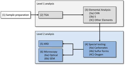
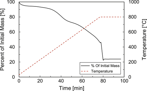
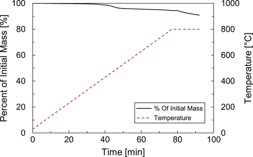
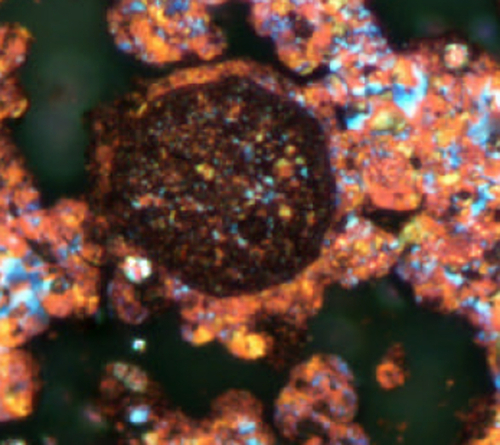
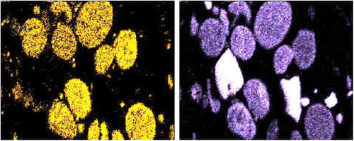
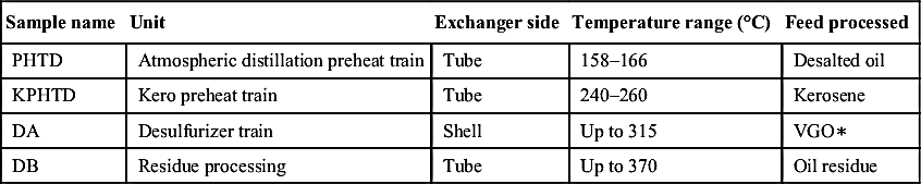
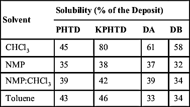
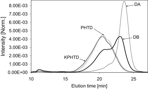
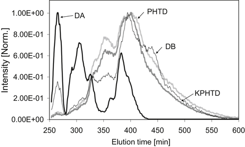
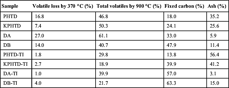

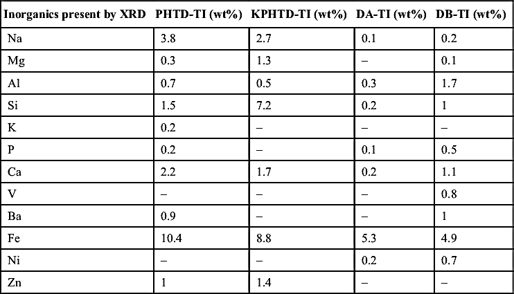
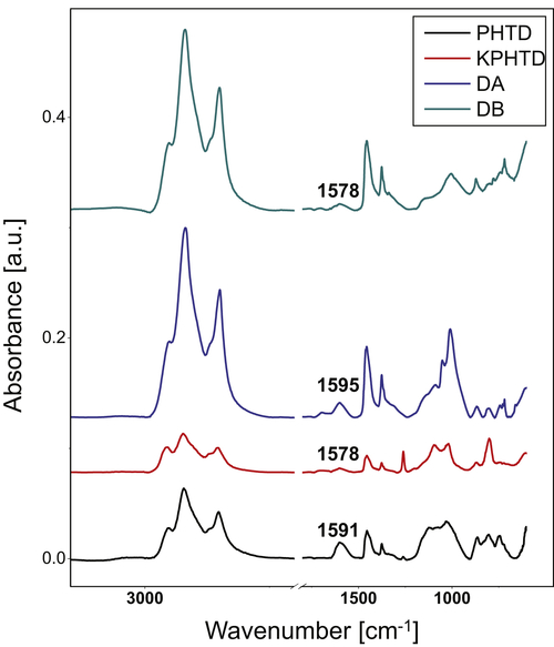
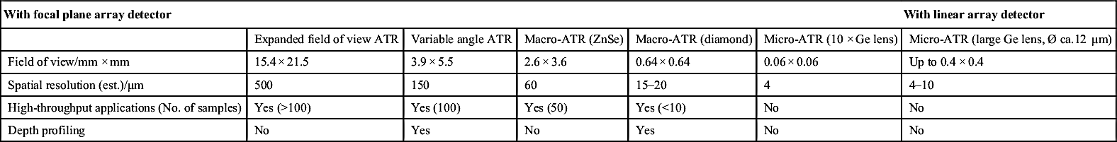
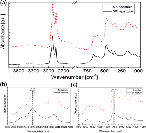
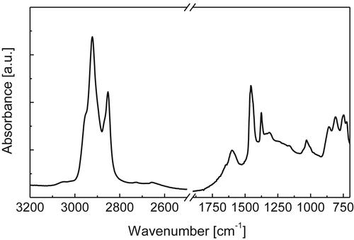
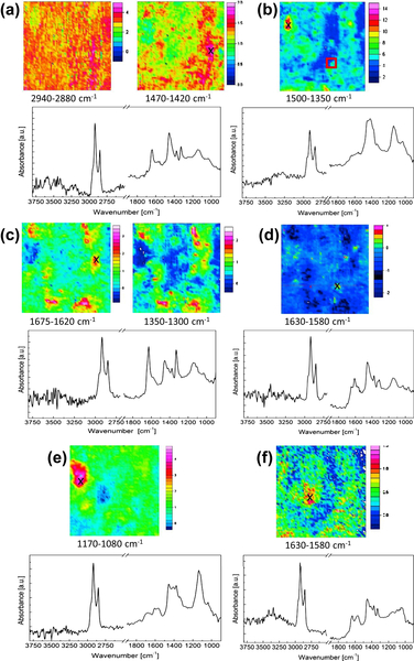
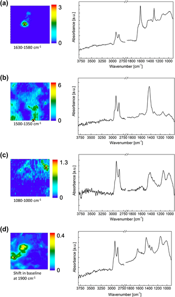
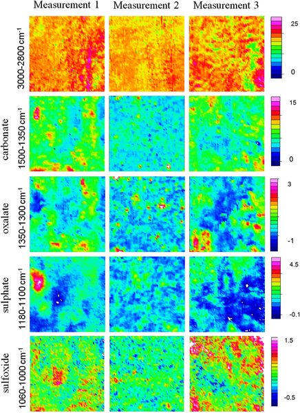
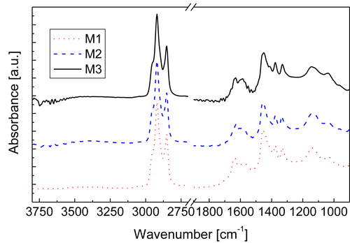
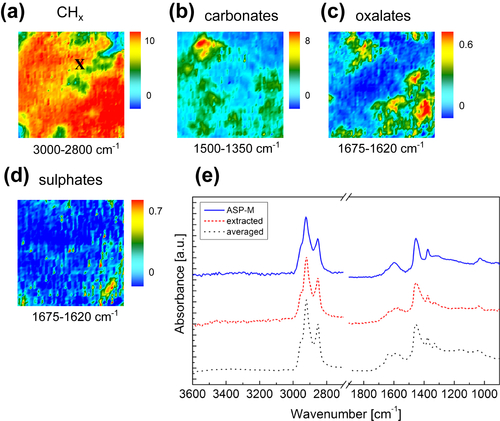
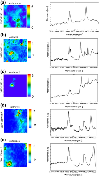
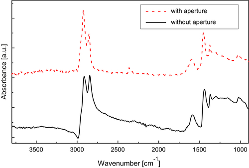
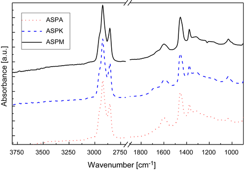
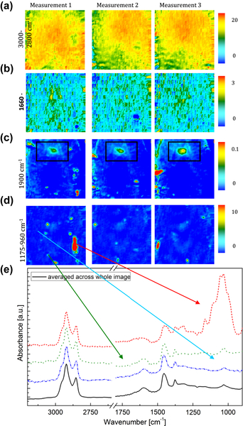
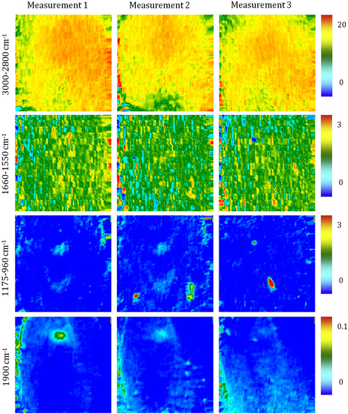
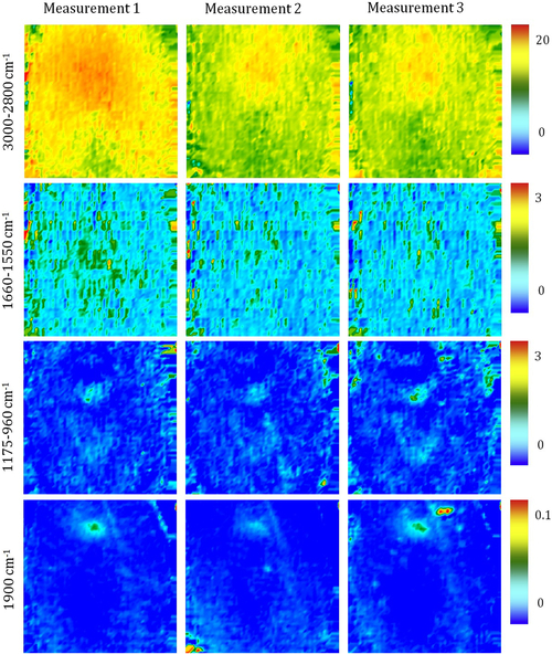
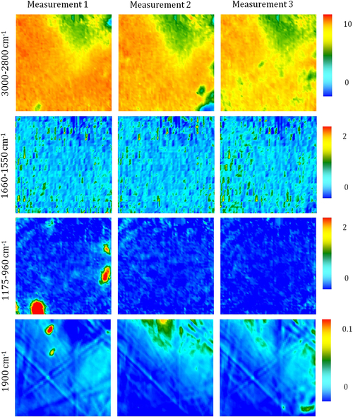
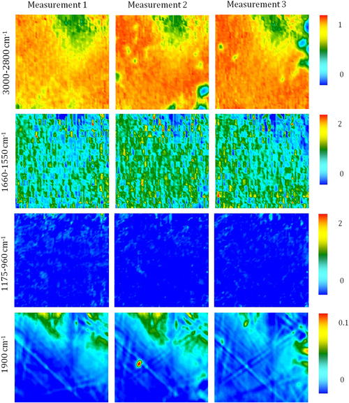
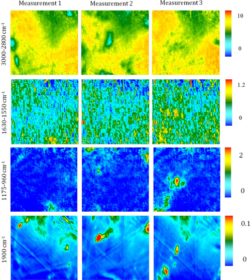
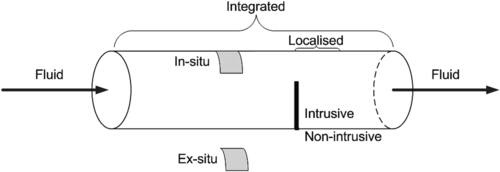
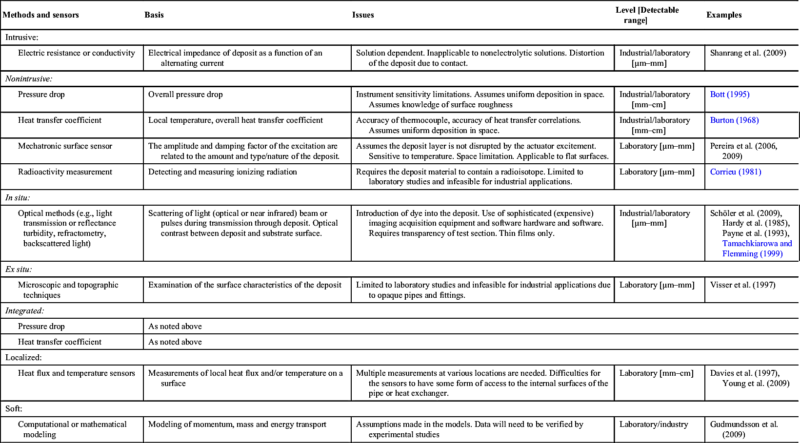
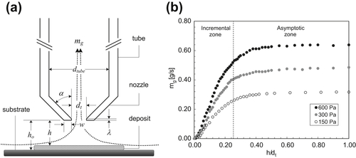
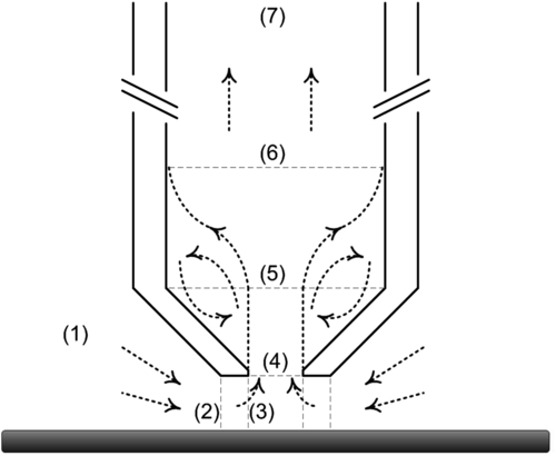
 (4.4)
(4.4) (4.5)
(4.5) (4.6)
(4.6) (4.7)
(4.7)