
5.2. Thermodynamic and Molecular Modeling
G. Jimenez-Serratos, A. J. Haslam, G. Jackson, E. A. Müller
Despite considerable efforts both from the scientific and the industrial community, most efforts at mitigating both asphaltene precipitation and fouling are based on an empirical and heuristic knowledge. As compared to other fields, such as bioindustry, fine chemicals, or polymers, the fundamental knowledge of the physico-chemical processes associated with oil and gas production is lagging far behind. Much of the fault lies in the current inability to fully characterize the working fluids and the simple impossibility of accounting for a full molecular description of a mixture of tens of thousands of distinct components with wide distributions of sizes and weights and whose complex interactions are difficult to understand. Molecular thermodynamics and statistical mechanics are the pillars of any modern description of the phase behavior of these complex systems. Special note is made of the contribution that computational simulations at different length scales can make to the understanding of the intricacies of this problem. The uniqueness of the problem and the lack of clarity in the methodologies that must be used have allowed the coinage of the distinct scientific discipline of “petroleomics” as the attempt to link molecular structure and the observed behavior (Breure et al., 2013).
5.2.1. Introduction
The complexity of a petrochemical mixture is such that a description based on the accounting of the individual distinct chemical species is simply impossible. Hence, diverse strategies have been suggested to reduce the unmanageable number of degrees of freedom by reducing the number of components considered in the model, by “lumping” groups of molecules with similar mass and chemical behavior into pseudocomponents, which are then treated classically. A more elegant approach is the consideration of a nonclassical treatment in terms of continuum thermodynamics (Cotterman et al., 1985; Cotterman and Prausnitz, 1985; Jaubert et al., 2000). Although this is an excellent conceptual approach, its implementation has not been widespread, presumably due to the reluctance of researchers and industry to modify the existing models to any large extent and particularly to make changes to software to account for a different approach to solving the phase equilibria. Most approaches to describing oil and gas mixtures make use of the idea of simplifying the mixture into pseudocomponents, the number of which depends on the application, but may vary from two, as in the black-oil–water models common in reservoir simulations to typically several dozen, as in equation-of-state modeling of light condensates. One should note, however, that studies with over 100 pseudocomponents have been reported (Avaullee et al., 1997). A common lumping criterion for classifying compound types instead of individual compounds is the SARA analysis method, in which four fractions are distinguished: saturates, aromatics, resins, and asphaltene. A key problem in the description is the characterization of asphaltenes, which are polyaromatic, heavy, and polar components considered the major precursors of sediments. In terms of solubility, asphaltenes are defined as soluble in aromatics like benzene and toluene but insoluble in alkanes like n-pentane and n-heptane (Ortega-Rodríguez et al., 2004; Pedersen and Christensen, 2006; Ancheyta et al., 2010; Artola et al., 2011; Breure et al., 2013; Ungerer et al., 2014).
Any attempt to gain a working knowledge in the field must inevitably consider the prediction of the behavior of the system as a function of temperature, pressure, and composition through modern thermodynamic tools involving the molecular description of the crude-oil components, the understanding and modeling of their intermolecular forces, and the ultimate integration of this information in the form of a (hopefully) closed-form equation of state (Aguilera-Mercado et al., 2006; Ancheyta et al., 2010; Artola et al., 2011; Ungerer et al., 2014). As simple as the previous statement might sound, the issue of constructing an equation of state has been a considerable challenge and is the subject of this section. Particularly, from a theoretical perspective, equations of state (EOS) are reliable tools for predicting the phase diagram and precipitation behavior. Although thermodynamic treatments of this problem date back as far as the late 1970s and early 1980s, the problem is as yet far from being resolved. The aim of this section is to give an overview of the platforms that thermodynamics and molecular modeling offer to contribute to the understanding of petroleum industry problems and particularly of the precipitation of asphaltenes and the consequent fouling.
5.2.1.1. Molecular Models of Asphaltenes
To be able to model appropriately systems containing fractions (such as asphaltenes) that may precipitate out of solution, it is vital to have an accurate description of the molecular structure. This in itself is a very challenging step as asphaltenes represent a solubility class of molecules, rather than a distinct molecule. As described earlier, an assumption must be made that there is a representative molecule or group of molecules that have chemical characteristics similar to those of asphaltenes and be can be used as a proxy for the description of a continuum of asphaltene molecular structures. It is not the intention of this review to give a detailed examination of the literature concerning asphaltene molecular structure. Two recent reviews give an overview of the available experimental data and the contentions regarding the size of the aromatic core and the corresponding molecular weight (Mullins, 2011; Herod et al., 2012).
As already noted in Chapter 2, in the case of asphaltenes and resins, there is no precise molecular formula or structure because by definition, a range of compounds falls into each of these categories and they invariably vary from crude to crude (Gray et al., 2011; Breure et al., 2013; Ungerer et al., 2014). Asphaltenes are usually defined operationally to be the (toluene soluble) fraction precipitated from oil on the addition of n-heptane; however, analogous precipitation from the oil can also be induced by the addition of other precipitants or, in particular, by changes in the thermodynamic conditions (temperature and/or pressure); such precipitates are also often referred to as asphaltenes. The detailed properties of these components are far from being well understood, and even their molecular weights are the subject of controversy (Mullins et al.; 2008; Herod et al., 2008). In the case of asphaltenes, polydispersity and solvent conditions affect the estimates giving numbers that realistically range from 700 to 3000 g mol−1 for asphaltenes (Aguilera-Mercado et al., 2006; Ancheyta et al., 2010). Some trends in the precipitation of asphaltenes have nevertheless been found in terms of general molecular properties, such as C/H ratio or the aforementioned molecular-weight range.
Molecular models for asphaltenes are sorted into three prototypical categories: continental, island, and archipelago. In the continental model, asphaltenes are represented with aromatic cores with some aliphatic branches; the island model has a similar structure and C/H ratio but a lower molecular weight (with a vague separation between both models); and the archipelago model consists of small aromatic regions bridged by alkanes (Ancheyta et al., 2010; Wiehe, 2012; Ungerer, 2014). Each model can stack differently, which can be useful for modeling specific behavior. It is likely that most crudes will have a combination of these structures, with possibly a predominance of a particular one. A vast fauna of supramolecular formations is reported in the literature: stacking of molecules into clusters, fractal aggregates, liquid-crystal domains, micelles, fibers, tubes, gels, and porous materials (Sirota, 2005; Gray et al., 2011; Breure et al., 2012). Experimental efforts using techniques such as small-angle neutron scattering, small-angle X-ray scattering, X-ray diffraction, nuclear magnetic resonance, and dynamic light scattering have helped to understand the structure and aggregation of asphaltenes (Pedersen and Christensen, 2006; Ancheyta, 2010), but the problem still resembles that of the Hindu fable retold by Saxe (1872) of the attempt of blind men to describe an elephant (Figure 5.6).

Intermolecular interactions are a key factor in the description of asphaltene-containing systems. As described early on by Murgich (2002), the list includes acid–base interactions, hydrogen bonding, formation of charge-transfer complexes, apolar associations, and π–π stacking. The relative importance of the different types of interactions in typical heavy oils and aslphaltenes is far from clear (Gray et al., 2011), again despite the crucial importance of these interactions as drivers for precipitation. The use in experiments and at theoretical level of proxies or pseudofluids which might represent a fraction of crude oil with simpler or better defined molecules trying to resemble the intermolecular interactions or behavior of the mixture has been attempted (Sirota, 2005; Gonzalez et al., 2007; Artola, 2011; Greenfield, 2011; Breure et al., 2012). Examples of molecules that can be used as pseudocomponents to represent asphaltenes are polystyrene and hexa-tert-butyl hexa-peri hexabenzocoronene. These molecules share fundamental characteristics with asphaltenes: they contain aromatic and aliphatic structures and have similar solubility properties (Sirota, 2005; Artola, 2011; Breure et al., 2012).
5.2.1.2. Aggregation Models
One of the existing theories for asphaltene aggregation suggests that the dominant role in the aggregation process is the interplay between asphaltenes and resins. Polar regions of resins and asphaltenes would exert attractive forces by hydrogen bonds or dipole–dipole interactions (Ancheyta et al., 2010). Following this line of thought one would have to recognize resins as stability agents preventing asphaltene deposition. Under such a description, asphaltenes are considered as micelles or colloidal systems surrounded by resins that screen the interactions with the aliphatic compounds in the solvent (because resins are soluble in n-heptane, contrary to asphaltenes) (Pfeiffer and Saal, 1940; Pedersen and Christensen, 2006; Pina, 2006; Ancheyta et al., 2010). Presumably, if there is a lack of resins, the micelles attract each other forming bigger structures. Consequently, the resins/asphaltene ratio is found to be a decisive factor for the stability of petroleum (Pfeiffer and Saal, 1940; Ancheyta et al., 2010). However, other authors claim that a direct relation between the resin/asphaltene ratio cannot be established as there is a dependency on saturates content that must be considered (Buenrostro-González et al., 2001). Furthermore, other tests have revealed stability or instability effects of resins, depending on the nature of the crude (Pereira, 2007). An interesting overview of the contrasting descriptions is given by Ancheyta et al. (2010).
The micellar model can be traced to work of the 1920–1940s (Nellensteyn, 1923; Pfeiffer and Saal, 1940) and its historic persistence over the intervening years (Fahim et al., 2001) is a testament of the capacity of the model to explain complex observations. However, from a conceptual and fundamental point of view it is inaccurate as asphaltenic systems do not exhibit a critical micellar concentration or the expected bimodal behavior of the distributions of aggregate sizes (namely, one peak related to actual micelles and the other one to individual amphiphiles, in the case of surfactant systems) (Sirota, 2005; Aguilera–Mercado et al., 2006; Pedersen and Christensen, 2006). Well-known variations of these micellar/colloidal models are the Yen (renamed Yen-Mullins) model (Buenrostro-González et al., 2001; Mullins, 2010). Under such conception, asphaltenes are assumed to form nanoaggregates from the stacking of aromatic sheets and then those aggregates form larger clusters defining a hierarchical organization (Mullins et al., 2007; Mullins, 2008; Wiehe, 2012). Again, some statements disproving the conceptual basis of colloidal models can be found in the literature. As an example, Sirota (2005) argues that even the interpretation of scattering experiments assuming asphaltenes as particles can lead to a misunderstanding of phase separation scattering data. Another interesting point is the precipitation exhibited in asphaltenic systems at high temperatures. In the colloidal model resins are expected to respond to the temperature increase by mixing in the solvent destabilizing the asphaltenes, but according to Sirota (2005) this explanation is inconsistent because the difference in molecular weight between asphaltenes and resins to reproduce such behavior should be larger than the experimental estimates.
A more-modern line of thought aims at describing the aggregation as a liquid–liquid phase separation. Even in the case of “athermal” systems, the interactions play a secondary role and it is the asymmetry in sizes that leads to the driving force in precipitation processes (Frenkel and Louis, 1992). This in itself is not sufficient to describe all the features of the aggregation process, but is definitively an important driving force. The description of the problem may be made in the context of solution theory of molecules, where asphaltenes are not assumed to be suspended but dissolved in the oil and the precipitation is seen as a phase separation process (Sirota, 2005; Pina et al., 2006). Solubility models of this type are typically based on the Flory–Huggins theory for polymer solutions (Flory, 1941; Huggins, 1941); at this level, resins are not typically considered an explicit component, having a less-relevant function than in colloidal models (Hirschberg et al., 1984; de Boer et al., 1995; Wu et al., 1998). A glass transition phenomenon as a possible model has also been suggested (Sirota, 2005).
5.2.2. Thermodynamic Approaches
From the abridged discussion presented in the previous sections, it is obvious that there is a fundamental lack of physical insight into the asphaltene deposition problem and the modeling lags behind because of this. This is not to say that there have not been a large number of attempts to develop a consistent and workable theory. The unique nature of the problem requires, however, a unique tailor-made methodology. Instead, most current attempts to model these mixtures are based on the adaptation of current techniques used to model surfactants, polymers, colloids, and/or the phase equilibria of simple mixtures. The resulting strategies fail mainly because of this lack of correspondence between the real problem modeled and the forced idealization of theoreticians.
Experimental research constitutes the central mechanism for understanding the behavior of crude oil and conditions for asphaltene precipitation. Improvements in the technology over the last decades have provided enhanced experimental data under extreme conditions and with higher sensitivity (Mullins et al., 2007). However, complications related to data analysis, operational cost, control of experimental conditions, and in general, the ultimate aspiration of establishing predictive connections between the characteristics of the mixture and the phase behavior require the use of theoretical and computational approaches. The petroleum industry is an innate and demanding consumer of thermodynamic tools for the description of the phase behavior of crude oil and related systems (Kontogeorgis and Folas, 2010) and this has been instrumental in the developments of recent years.
Semiempirical methods, correlations, and engineering-type correlative procedures represent a basic attempt to characterize pressure–temperature–composition behavior of pure compounds or mixtures of industrial interest. However, the complexity of the system of interest leads to numerous empirical adjustable parameters and correlations that do not possess a clear physical meaning (Ortega-Rodríguez et al., 2004; Aguilera-Mercado et al., 2006; Pedersen and Christensen, 2006). Empirical cubic equations of state, molecular-based thermodynamic theories, and their combination with computer simulations represent useful alternatives for characterizing the system from a physical perspective. In particular, a statistical thermodynamic approach gives a further connection between the structural features and the corresponding macroscopic properties (Pedersen and Christensen, 2006; Mullins et al., 2007). Herein some of the most common and successful of such thermodynamically based approaches will be discussed.
5.2.2.1. Polymer Solution Models
As noted previously, Flory–Huggins (FH) polymer solution theory has been recurrently used to model precipitation of asphaltenes in combination with the Hildebrand regular solution theory (RST) (Hildebrand, 1929; Hildebrand et al., 1970). In the framework proposed by Hirschberg et al. (1984), a mixture of asphaltenes, maltenes, and liquid can be represented as a simple binary system wherein the asphaltenes are one of the components and the maltenes and liquid the second component. The maximum volume fraction of asphaltenes soluble in the oil phase assumes the form (Hirschberg et al., 1984; Pedersen and Christensen, 2006):
 (5.48)
where Rg is the universal gas constant, T is the temperature, VL and VA are the molar volumes of the asphaltenes in the liquid and asphaltene phases, respectively, and δL and δA are the average solubility parameters of the nanoaggregates or asphaltenes in the corresponding component of the binary mixture. These authors note that the main weakness of their model is that it excludes the effect of resins. An implicit way to incorporate this is by modifying the asphaltene solubility to higher values in the liquid phase than that of pure asphaltene. In the same work, the vapor–pressure equilibrium is solved by using the Soave–Redlich–Kwong (SRK) cubic EOS, but there is a thermodynamic inconsistency as the solution is not unique (Pedersen and Christensen, 2006).
As can be seen from Equation (5.48), the amount of asphaltenes in solution strongly depends on the average solubility parameter. Further modifications by other authors include better estimates of the average solubility parameter of the oil, e.g., the study of Wang and Buckley (2001), where a correlation with the refractive index is used.
Alboudwarej et al. (2003) have obtained a qualitative description of precipitation in Athabasca bitumen using a more-sophisticated model. The author included n-paraffin, saturates, aromatics, resins, and asphaltenes as pseudocomponents of the mixture; the asphaltenes (considered with a molecular-weight distribution) and resins populate the asphaltene-rich phase.
Other notable studies employing lattice models are those of Burke et al. (1990), Kawanaka et al. (1991), Kokal et al. (2003), and de Boer et al. (1995). For example, Kawanaka et al. (1991) used an extension of the Flory–Huggins polymer solution theory, developed by Scott and Magat to incorporate the effect of polydispersity through heterogeneous distributions of polymers (Scott and Magat, 1945; Scott, 1945).
Considering the complexity of asphaltenes and crude oils, it is remarkable that simple descriptions like the FH-RST can offer a suitable qualitative description of the precipitation phenomenon. Importantly, these models are not predictive and the parameters must be obtained from experimental data (Kontogeorgis and Folas, 2010). The deficiencies of these theories come from deep features of the system that require more complete characterizations: the association phenomena of asphaltenes with resins, the description of the asphaltene–oil equilibria (is it a liquid–liquid, solid–liquid, colloidal instability?), the extensive association in the components of the mixture, etc.
For the interested reader, a rich discussion on the Flory–Huggins solution model applied to bituminous systems is made by Wiehe (2012) and a recent and detailed review is presented by Forte and Taylor (2014). The foundations of these approaches and their applications to other systems can also be gleaned from Kontogeorgis and Folas (2010).
5.2.2.2. Cubic Equations of State
Cubic equations of state are classical models for systems at pressures high enough so that the intermolecular interactions have a significant effect on the vapor–liquid equilibrium (VLE), i.e., nonideal conditions (Kontogeorgis and Folas, 2010). Bernoulli at the end of the eighteenth century proposed the inclusion of the volume of the molecules as a repulsive term, but it was van der Waals (vdW) and works derived from his doctoral thesis in 1873 that resulted in the EOS that accounts for such a repulsive contribution and a pressure correction related to attractive forces (van der Waals, 1873; Valderrama, 2003). Although the vdW EOS is not quantitatively accurate for most applications, the prediction of a critical point and the description of vapor–liquid coexistence below the critical point represented a giant leap in the representation PVT behavior. The vdW equation and the countless modifications can be written as a generic cubic equation (Valderrama, 2003):
 (5.49)
where a, b, c, and d are constants or functions of temperature, acentric factor, critical compressibility, etc. The third degree in the volume V gives a simple mathematical form and the extension to mixtures is relatively direct.
Modifications to vdW EOS that keep the cubic dependence in volume usually change the attractive pressure term of Equation (5.49). The original work of Redlich-Kwong (1949) proposed an attractive term which is temperature dependent through a function α(T) and opened up the field for a myriad of different empirical versions of this attractive term; it was rapidly understood that it was this second term in Equation (5.49) that carried all the important weight into the parameterization of fluid phase equilibria. Wilson (1964) introduced Pitzer’s acentric factor, α(TR,ω) as a third parameter in the parameterization and Soave (1972) improved the functional definition of the α(TR,ω) function. The Peng-Robinson (1976) modification consists of improvements to Soave’s version by changing the form of the attractive term and recalculating the α(TR,ω) function (Kontogeorgis and Folas, 2010). Further versions usually follow three approaches (Valderrama, 2003): a modification of α(TR,ω); a modification of the volume dependence of the attractive term (or both by applying volume translations, Peneloux et al., 1982); and the use of a third substance-dependent parameter. Numerous variations and the efforts to improve mixing and combining rules result in a wide tailor-made suite of cubic EOS to describe diverse systems. Kontogeorgis and Folas (2010) and Valderrama (2003) present well-organized information and tables that summarize the wide variety of cubic EOS in use today.
In the field of asphaltenes, two major approaches have been used. The first is to group the mixture into a reduced number of pseudocomponents and describe each with specific critical properties. The second is to describe properties through continuous distributions to represent the reservoir mixture (Haynes and Mathews, 1991; Vakili-Nezhaad et al., 2001).
Yarborough used the PR-EOS (1979) to predict the fluid-phase behavior of crude oils and gas condensates. In his study, a procedure to characterize heptanes and heavier components was developed and comparisons of calculated and experimental VLE for ternary systems were made. Contemporary contributions to that of Yarborough are those of Vogel et al. (1983), Willman and Teja (1987), Firoozabadi (1988), and Skjold-Jørgensen (1984).
The Peng-Robinson EOS was used by Szewczyk and Béhar (1999) to study flocculation, considering it as the appearance of a second liquid phase. The mixture has three components: C10–, C10–20, and C20+ fractions. For pressures above the bubble pressure, flocculation appears as a liquid–liquid separation, while under the bubble pressure, there is a liquid–liquid–vapor equilibrium. The main problem in this study is (as is usual in modeling approaches) the large number of parameters required and the difficulty of obtaining them, which is an obstacle to implementation at an industrial level (Pina et al., 2006).
In the work of Nghiem et al. (1993) the PR-EOS was used to model the gas and liquid phases, whereas the asphaltene phase was considered to be a pure solid, the fugacity of which is given as function of temperature, pressure, and the asphaltene onset pressure. In a related work, Kohse et al. (2000) model the mixture with 12 pseudocomponents, where the asphaltene is again modeled as a pure solid. The solid model is also the basis of the work of Jamaluddin et al. (2000) and Castellanos Díaz et al. (2011) in which the complexity of the representation is increased, including 17 components in the first case and 16 to represent the boiling-point curve in the latter.
Examples of applications of EOS to asphaltene precipitation where a large number of compounds or pseudocompounds are included in the models are those of Sabbagh et al. (2006) and Behar et al. (2003) that use of the order of 30 to model bitumen, using the PR-EOS (Forte and Taylor, 2014).
In the context of gas-injection modeling, a comparative study by Danesh et al. (1991) analyzed and compared the phase behavior and volumetric properties of injection gas-reservoir oil systems obtained through cubic EOS. They concluded that the modified Patel-Teja (VPT) (1982) and the Zudkevitch-Joffe-Redlich-Kwong (ZJRK) EOS (Zudkevitch and Joffe,1970) were generally superior to other approaches, that the inclusion of the volume-translation concept improves the liquid density prediction, and that all of the tested EOS needed pertinent experimental information to be reliably used close to miscibility conditions.
Victorov and Firoozabadi (1996) proposed a description under the micellar model; the petroleum was assumed to be a dilute solution and the PR-EOS was applied to calculate the fugacity of monomeric asphaltene in the bulk of the petroleum fluid. The model captures the change in precipitation for different precipitants and it is sensitive to the quantity of resins in the mixture. Following the micellar model other works include that of Pan and Firoozabadi (1998), Fahim et al. (2001), and Mahdavi and Kharrat (2011), among others (Forte and Taylor, 2014).
The success of cubic EOS in the petroleum industry is based on their simplicity, which is suitable for fast calculations of relevant mixtures. However, even when they can provide accurate correlations, their predictive power can be restricted to some intervals of phase space (Artola et al., 2011). As the mixtures and corresponding interactions increase in complexity, cubic EOS present severe limitations. Polarity, associative features, and the large asymmetry in the molecular sizes involved are some of the aspects that cannot be included in an appropriate manner with a cubic EOS (Kontogeorgis and Folas, 2010; Artola et al., 2011). Increasing the predictive power of cubic EOS for multicomponent and multiphase mixtures containing hydrocarbons and polar/associating chemicals was the practical motivation of the development of the Cubic-Plus-Association EOS (Forte and Taylor, 2010; Kontogeorgis and Folas, 2010).
5.2.2.3. The Cubic-Plus-Association Equation of State
The Cubic-Plus-Association EOS (Kontogeorgis et al., 1996) is a combination of the SRK equation (although other cubic EOS can be used) with an association term, based on the Wertheim first-order perturbation theory (1984a, 1984b, 1986a,b) of the type used in the statistical associating fluid theory (SAFT), described later in Section 5.2.2.4. As presented by Kontogeorgis et al. (1996, 1999), the associative effect is introduced as
 (5.50)
where ρ is the molar density (=1/V) and  is the fraction of nonassociated molecules, which depends on the association strength between two sites belonging to two different molecules, given in terms of the radial distribution function g. A complete exposition of the general theory, details of the combination and mixing rules, and industrial applications has been given by Kontogeorgis and Folas (2010).
In the oil and gas industry, the introduction of associative effects finds a natural market. Applications of CPA-EOS to asphaltene precipitation can be found in the recent work of Li and Firoozabadi (2010a,b). In the first case the authors study asphaltene precipitation in model solutions (asphaltene + toluene) and in heavy oils and bitumens. The system is characterized through three pseudocomponents including saturates, aromatics/resins, and asphaltenes. The PR-EOS is the basis of the method and the associations between asphaltenes and those between asphaltenes and heavy components are contemplated with the Wertheim association term. The model describes the saturation and onset pressures, the amount of asphaltene precipitated, and the gas–liquid–asphaltene behavior for several live oils. In the second study the precipitation is modeled again as liquid–liquid or gas–liquid–liquid separation. The pseudocomponents of the mixture are: pure components, pseudohydrocarbon components, and the hydrocarbon residue, which is further divided into “heavy” (alkanes, heavy aromatics, and resins) and asphaltene. A successful description of the effect of pressure and temperature on the bubble point is reported, as well as the phase separation behavior. Shirani et al. (2012) have used PR and SRK EOS to describe the physical part of the interactions, and the association contribution is attributed to chemical interactions and hydrogen bonding. The model is based on the Whitson’s splitting and lumping method (Ahmed, 1989), and the asphaltenes are considered as molecules with two association sites. The SRK description is found to be superior to that of PR-EOS when compared with experimental data for live oils.
Including molecular information in the thermodynamic description enables the connection between the structure (microscopic) and the function (macroscopic), contrary to pure macroscopic approaches (Ortega-Rodríguez, 2004; Prausnitz and Tavares, 2004). Although the equations of state discussed are useful tools for the modeling of asphaltene-deposition behavior, their parameters do not permit the aforementioned link to be established and follow the trail of the intermolecular potentials. On the other hand, models based on statistical thermodynamic theories, such as statistical associating fluid theory (SAFT, described in the next section), include parameters with a well-defined physical meaning (Müller and Gubbins, 2001; Kontogeorgis and Folas, 2010).
5.2.2.4. Statistical Associating Fluid Theory Equation of State
Based on statistical thermodynamics, Wertheim (1984a,b, 1986a,b) developed a first-order perturbation theory for the free energy of fluids with a repulsive core and strong directional short-range attractive sites. In the SAFT approach, as presented by Chapman et al. (1988, 1989, 1990), molecules are modeled as spheres (monomers) or chains of fused spheres with associating sites. The Helmholtz free energy is given as separate terms: the ideal term; the contribution from monomeric repulsive or dispersive interactions; the contribution due to formation of chains; and the contribution due to association. In general, when considering crude oils, the association term is dropped and the equation related only to terms linked with the underlying “monomers” and the chain length, m.
The original SAFT EOS has been adapted to describe a complex system with particular features. This flexibility gives SAFT key advantages over common cubic EOS. Some of the well-accepted versions of SAFT (Kontogeorgis and Folas, 2010) are the following: CK-SAFT (Huang and Radosz, 1990, 1991), Simplified SAFT (Fu and Sandler,1995), LJ-SAFT (Kraska and Gubbins, 1996a,b), SAFT-VR (Gil-Villegas et al., 1997; McCabe et al., 1999), Soft SAFT (Blas and Vega, 1998), PC-SAFT (Gross and Sadowski, 2001), Simplified PC-SAFT (von Solms et al., 2003; Tihic et al.,2006), and the recent and versatile SAFT-VR Mie (Lafitte et al., 2013) and SAFT-γ (Papaioannou et al., 2014). Reviews of the SAFT methodology and more details about the versions can be found in Müller and Gubbins (2001), Economou (2002), Kontogeorgis and Folas (2010), and McCabe and Galindo (2010).
The use SAFT in modeling alkane and oil-like systems is now well established in the oil industry (Leekumjorn and Krejbjerg, 2013). In particular, SAFT has been applied with some success in modeling the onset of asphaltene deposition from crude oil (Wu et al., 2000; Tan et al., 2008; Punnapala, 2013; Sedghi, 2014). Special mention is due to the efforts of the Chapman group at Rice who have a particularly exhaustive set of papers on the different aspects of modeling asphaltene systems with the SAFT EOS (Ting et al., 2003; Gonzalez et al., 2005, 2007, 2008; Vargas et al., 2009a,b; Panuganti et al., 2013). By capturing experimental onset and bubble-point data, these studies have demonstrated the broad applicability of SAFT for the study of crude-oil systems.
Among the biggest challenges present in applying SAFT is the description of the asphaltene fraction; i.e., what is the molecular description of an asphaltene? The nature of the SAFT EOS allows only for a description in terms of distinct energies and molecular sizes, so there is very little justification for the use of a large number of adjustable parameters. The extent of the capabilities of a SAFT calculation in which most of the different components of the crude oil share the same parameters (distinguishing themselves by the different average chain lengths for each pseudocomponent fraction) is shown in Figure 5.7. The asphaltene fraction is treated as a single component and a single binary interaction parameter is employed to describe the experimental data (Artola et al., 2011).
The general trends of the experimental data are clearly reproduced. The bubble curve is seen to be the boundary delimiting a three-phase region of VLLE, while the location of the precipitation boundary is strongly related to the LLE boundary, clearly supporting the interpretation that the onset of precipitation of the asphaltene can be represented as a liquid–liquid instability. In addition, one can understand how the precipitation boundary would be affected by changes in the nature of the crude oil. Of course, it is important to bear in mind that in reality, the precipitation boundary would be very sensitive to the precise distribution of asphaltenic species and not just the average molecular weight. For example, a sample with a long-tail distribution of larger molecules would be more prone to be unstable than a system with an equivalent average molecular weight, but a sharper distribution; such sensitivity is well known in polymer–solvent phase equilibria.
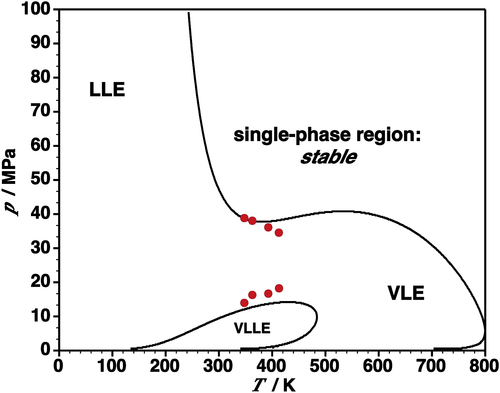
The crude-oil bubble curve is essentially that of an asphaltene-free liquid phase; i.e., in terms of the light (or oil) components, the composition of the two liquids inside the two-phase liquid–liquid (LLE) region is essentially the same. By contrast, if one considers instead the composition of the asphaltene, a marked difference in the phases is found; at low pressure two phases are present, one in which the mole fraction of asphaltene is close to unity, and one (a gaseous phase) in which there is, essentially, no asphaltene. At c. 3.5 MPa, a third phase appears in which there is still very little asphaltene. In this three-phase region, the content of lights in the liquid phases increases with pressure, while that of the heavier components decreases accordingly. At higher pressure, once again only two phases are observed and although asphaltene is present in both phases, the composition of asphaltene in the asphaltene-rich phase remains at least an order of magnitude higher than that in the other phase. This analysis of the two phases, one of them largely free of any asphaltene, provides a physically relevant picture of the phase behavior.
5.2.3. Molecular Modeling as Applied to Crude Oils
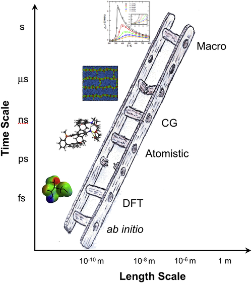
The options available to describe the behavior of matter in silico resemble a ladder (Figure 5.8), where each of the steps from the bottom up can be thought as representing different scales of ever-decreasing physical detail.
At the bottom of the ladder is the full electronic quantum mechanical description of matter: essentially exact numerical solution of the Schrodinger equation for the many-body wavefunction, using, for example, configuration interaction or renormalization group methods. This is only feasible for a handful of atoms at most because the complexity of the many-body wavefunction increases exponentially with the number of particles. If one is willing to accept a few simplifications, density functional theory (DFT) offers a very successful combination of accuracy and relatively low computational cost, and makes it possible to run simulations on hundreds of atoms as a matter of routine, and thousands of atoms on large supercomputers (Burke, 2012). Though DFT has become a widely accepted tool it is burdened with two important consequences of the inherent simplifications: the use of more complicated wave functions do not necessarily provide more accuracy and there is no rigorous way of accounting for dispersion forces within a DFT treatment, which for an accurate description of fluid-phase equilibria is a crucial requirement. Larger scales must be sought. Up a rung of the ladder is a description of atoms or tightly bound chemically distinct groups, such as the CH3 and CH2 groups of n-alkanes, using the simpler force fields of classical mechanics, which are commonly represented with spherical symmetrical pair potentials with Coulombic charged sites. At this level of abstraction one therefore considers the interaction sites to be made up of a collection of atoms and atom groups or even small molecules, e.g., carbon dioxide or benzene. Such a methodology is commonly referred to a treatment at the coarse grained (CG) level. The intermolecular interactions at this CG level are typically described with semiempirical analytical functions of the interseparation taken to represent the pairwise potential energy, u(r). It is common practice to estimate the parameters of the force fields by attempting to reproduce target structural (radial distribution function, structure factor, etc.), thermodynamic (second virial coefficient, liquid density, vapor pressure, internal energy, enthalpy, etc.), or transport (viscosity, diffusivity, etc.) properties of the fluid or a combination of these properties. In an effort to resolve the dilemma of the degeneracy of macroscopic parameters for the intermolecular potential, it is then tempting to employ a more detailed, higher-resolution atomistic model (a step down the ladder) as the basis for determination of the parameters for CG models by means of an appropriate integration of the degrees of freedom which are to be removed. A review of current practice including a discussion of the key approaches to the simultaneous modeling of several time and/or length scales (multiscale modeling) is the subject of a book (Voth, 2009) and themed journal issues (Faller, 2009; Visscher et al., 2011). Also reviews on the topic have been published by Klein and Shinoda (2008), McCullagh et al. (2008), and Brini et al. (2013) to name just a salient few. It is at this level of abstraction that one may start envisaging the modeling of crude oils as the molecular level of representation must be coarsened with the complexity in order to allow for a tractable description of the molecular behavior. Models such as those employed to describe microphase separation, e.g., dissipative particle dynamics techniques (Groot and Warren, 1997), are representative examples of this next step up the ladder. These high-level CG models exhibit some of the consequences of the selective removal of degrees of freedom, echoed in issues of robustness, transferability, and representability. Further abstraction into more coarse grained models commonly removes all type of molecular descriptors and moves one into the realm of continuum models. The formal connection between these steps higher up our ladder is ever more sparse and very few models effectively bridge these gaps. This is an area of very dynamic and topical research.
5.2.4. The Combination of Equations of State with Molecular Modeling
While not the subject of this section, one could, in principle, attempt to obtain information and ultimately model the behavior of crude oils and gases through direct molecular modeling. A recent review by Greenfield (2011) summarizes the state of the art in terms of molecular modeling of asphaltene-containing crudes; unfortunately space limitations preclude any further discussion here. Molecular modeling of these systems is in itself is an immense challenge, as the difficulties present in equation-of-state modeling simply become enhanced, most importantly due to the finite size of the simulation sampling cell that must be used. However, very recently, a paradigm change has been proposed: the simultaneous use of an equation of state in conjunction with molecular modeling of fluids at the coarse-grained level (Müller and Jackson, 2014; Avendaño et al., 2011, 2013; Lafitte et al., 2012; Mejía et al., 2014).
Another important consequence of the simplicity of the SAFT approach noted in the previous section is that all of the component species are treated using models defined by integer values of the parameter m, which denotes the number of segments in the chain representing the molecule. Together with the low number of components in the model, this will allow the same system to be studied using molecular-simulation techniques, such as molecular dynamics. By contrast, had the crude-oil model comprised many components or (as would be usual in SAFT-type studies) any components would have been characterized by noninteger m (i.e., the model molecules consisted of a noninteger number of segments); such a complementary study would not be feasible.
Not all versions of SAFT have a direct link between the Hamiltonian and the final closed form EOS. A recent version of the equation denoted the SAFT–VR–Mie model (Lafitte et al. 2013) provides such a link in a tractable way. The direct molecular simulation of the SAFT molecular models provides a reliable route to properties that are not accessible from the equation of state such as the structure, the self-assembly into mesophases, the interfacial tension, the adsorption on surfaces, and the transport properties, all key to understanding the properties of asphaltenic systems. The group-contribution nature of the methodology (Papaioannou et al., 2014) allows for the description of the behavior of these complex fluids in a consistent and quantitative way. Furthermore, the one-to-one correspondence of the force fields to the equation of state provides a unique avenue to the multiscale modeling of crude oils.
5.2.5. Conclusions and Perspectives
The lack of a deep understanding of the physical phenomena leading to the instability of the fluid phase, aggregation, and posterior precipitation of asphaltenes is an open problem that is particularly important in crude-oil production, transport, and refining, because the economic cost associated with reservoir, pipeline, or heat exchanger fouling due to asphaltenes is substantial. Clearly, any insight into the precipitation phenomenon that could be provided by an improved understanding of the phase behavior of crude oil would be of great value, and this can be perceived as one of the principal goals of thermodynamic and molecular modeling.
Partly because of a paucity of experimental data, but also because the asphaltene fractions of crude oils are far from being well characterized, the problem of modeling crude-oil behavior from a thermodynamic perspective is as yet unresolved; it is this lack of a precise characterization that has represented the major barrier to improving our understanding in this area. Nevertheless, significant progress has been made; although a deep understanding remains some way off, studies such as those highlighted in this chapter have certainly provided useful and valuable insights. Within industry and academia there remains a substantial effort in continuing research both at the level of experimental characterization and in development of modeling techniques; together these promise continued improvement in our understanding of the important, yet perplexing, phenomenon of asphaltene precipitation.
..................Content has been hidden....................
You can't read the all page of ebook, please click here login for view all page.