5.4. Industrial Scale High-Fidelity Modeling

Search in book...
Toggle Font Controls
Create new playlist

Name your new playlist

Playlist description (optional)
Sign In

Email address

Password

Forgot Password?

or

Continue with Facebook

Continue with Google
Sign Up

Full Name

Email address

Confirm Email Address

Password

or

Continue with Facebook

Continue with Google

5.4. Industrial Scale High-Fidelity Modeling

F. Coletti and S. Macchietto

In Section 5.1 the current heat exchanger design methodologies and their limitations have been reviewed. This has highlighted the importance of integrating fouling models with thermal ones to capture adequately the different phenomena involved in the deposition of unwanted material on thermal surfaces. As recognized by Bott (1995b) the purpose of any fouling model is

“to assist the designer or indeed the operator of heat exchangers, to make an assessment of the impact of fouling on heat exchanger performance given certain operating conditions.”

To accomplish this goal, Schreier and Fryer (1995) noted that fouling models should take into account:

• The rates of the processes that lead to deposition.

• The temperature distribution and deposit thickness profile.

• The effect of flow on deposition and, if relevant, reentrainment (removal).

While Section 5.2 and Section 5.3 were concerned with improving underlying fouling models at a thermodynamic and fluid-dynamic level, this section focuses on the development and use of an industrial-level model for shell-and-tube heat exchangers undergoing crude oil fouling by Coletti and Macchietto (2011). This model integrates all the three aspects above and captures the thermal and hydraulic effects of fouling within refinery heat exchangers and preheat trains and is now implemented in Hexxcell Studio™, commercially available via Hexxcell Ltd.

The main features of the model are summarized as follows:

• Distributed heat balances are written in cylindrical coordinates where appropriate (i.e., for tube wall and fouling layer domains), which makes it possible to overcome the thin slab approximation—often used in the past—accounting for curvature effects of the heat exchanger tubes on the heat flux.

• The heat exchanger configuration is accounted for (e.g., number of tube-side passes, tube diameter and length, baffle spacing, pitch arrangement, etc.). The heat transfer coefficients and pressure drops on the shell-side are calculated using the Bell–Delaware method (Taborek, 2008a,b) or the flow stream analysis (Hewitt, 2008).

• Physical properties for both shell-side and tube-side fluids are considered as a function of temperature. API-based relationships are used as default model but other thermophysical property models (including company proprietary ones) can also be used if available.

• The Ebert–Panchal model (Equation (5.30)) used in a distributed (rather than lumped) way allows calculating the local value of fouling resistance at each point along the exchanger length as opposed to an average value for the whole exchanger.

• The growth of the fouling layer over time at any given point across the tube length is captured using a moving boundary approach. The corresponding reduction in flow radius, R_flow (the tube radius available for flow in actual fouled conditions), and restriction in cross-sectional flow area are calculated as a function of the fouling thickness, δ. Tube-side velocity (thus shear stress) and heat transfer coefficient are calculated as a function of R_flow.

• The structural changes of the fouling deposit over time are captured with the aging model by Coletti et al. (2010). This describes the changes in the thermal conductivity of the fouling layer at any point in the axial and radial direction as a function of the specific temperature history. More details on this model have been given in Section 5.1.5.1.

• An advanced equation-oriented process simulator that features an easy-to-use flowsheeting environment (gPROMS by PSE Ltd.) is used to solve the equations and estimate necessary model parameters. This framework has several advantages:

• It allows an easy setup of heat exchanger networks by interconnecting of individual heat exchanger units dragged-and-dropped in a flowsheet.

• The equation oriented architecture supports the solution of complex numerical problems and allows multiple types of calculations utilizing the same model.

• It is not a “black box.” In contrast to other tolls implemented in procedural programing language (e.g., c++ or Matlab), the architecture chosen here allows the user to easily access and modify model equations (e.g., fouling model), thus giving full control of the model.

• It allows the easy integration with other process models (e.g., distillation columns, controllers).

• It provides a unified framework that helps preventing “silos” between company functions allowing easy sharing of assumptions, validations, and developments among R&D, engineering design, operations.

The following sections will provide a summary of the model, its software implementation, the results, and applications that derive from its use.

5.4.1. Governing Equations

The model equations are reported in the original publication (Coletti and Macchietto, 2011). Here are briefly summarized the main equations of the thermal, hydraulic, and fouling models and their integration.

5.4.1.1. Thermal Model

One key feature of the Hexxcell model is that the underlying governing equations do not rely on averaged models such as the logarithmic mean temperature or the ε-NTU methods (Section 5.1.1). In the model by Coletti and Macchietto (2011), distributed heat balances are solved along the axial direction in each pass, n, of the heat exchanger:

$\frac{\partial}{\partial t} (ρ c_{p} T A_{f l o w}) = - d i r_{n} \frac{\partial}{\partial z} (ρ c_{p} T u A_{f l o w}) + \frac{\partial}{\partial z} (λ A_{f l o w} \frac{\partial T}{\partial z}) + α P ({T_{L} |}_{r = R_{f l o w}} - T)$ $\frac{\partial}{\partial t} (ρ c_{p} T A_{f l o w}) = - d i r_{n} \frac{\partial}{\partial z} (ρ c_{p} T u A_{f l o w}) + \frac{\partial}{\partial z} (λ A_{f l o w} \frac{\partial T}{\partial z}) + α P ({T_{L} |}_{r = R_{f l o w}} - T)$

(5.68)

where dir_n is a variable direction term, introduced to take into account the direction of the flow (dir_n = 1 in case of an odd pass, dir_n = –1 in case of an even pass). The fluid temperature, T, and its physical properties, ρ, c_p, λ, are a function of time, t, and spatial position, z, along the exchanger. The change in cross-sectional area of a tube caused by fouling is accounted for by considering the area of flow, A_flow, as a function of the fouling thickness, δ:

$A_{f l o w} = π R_{f l o w}^{2} = π {(R_{i} - δ)}^{2}$ $A_{f l o w} = π R_{f l o w}^{2} = π {(R_{i} - δ)}^{2}$

(5.69)

where R_flow denotes the flow radius and R_i the internal tube radius (Figure 5.38). The changes over time of the fouling layer thickness, δ, are calculated as a function of the local deposition rate, which, in turn, depends on the local value of the fouling resistance:

$\frac{d δ}{d t} = λ_{L}^{0} \frac{d R_{f}}{d t}$ $\frac{d δ}{d t} = λ_{L}^{0} \frac{d R_{f}}{d t}$

(5.70)

In Equation (5.70),

λ_{L}^{0}

$λ_{L}^{0}$

denotes the value of the thermal conductivity of the fresh deposits accumulating on the thermal surface whereas R_f is calculated according to Equation (5.77) below.

The effects of the restrictions caused by fouling buildup on the convective heat transfer coefficient, α, are also accounted for in Equation (5.68) by writing α as function of R_flow:

$α = \frac{λ N u}{2 R_{f l o w}}$ $α = \frac{λ N u}{2 R_{f l o w}}$

(5.71)

where λ denotes the fluid thermal conductivity and Nu is the Nusselt number, calculated through the Dittus–Boelter relationship (Hewitt et al., 1994). It can be noted that in Equation (5.71) the heat transfer coefficient is enhanced by the progressive reduction in cross-sectional area.

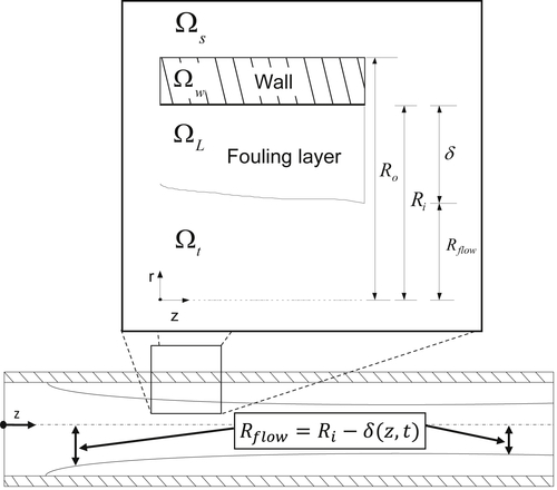
Figure 5.38 Main model domains and key geometrical quantities.

The fouling layer domain is represented as a two-dimensional conductive solid with a moving boundary defined a function of the thickness of the deposit growing in the heat exchanger tubes. Assuming negligible temperature gradients in the axial and angular coordinates and negligible heat of reaction from the aging process, the heat balance on differential segment of the fouling layer is

$δ^{2} ρ_{L} c_{p, L} \frac{\partial T_{L}}{\partial t} = \frac{\partial λ_{L}}{\partial \tilde{r}} \frac{\partial T_{L}}{\partial \tilde{r}} - \frac{λ_{L} δ}{R_{i} - \tilde{r} δ} \frac{\partial T_{L}}{\partial \tilde{r}} + λ_{L} \frac{\partial^{2} T_{L}}{\partial {\tilde{r}}^{2}}$ $δ^{2} ρ_{L} c_{p, L} \frac{\partial T_{L}}{\partial t} = \frac{\partial λ_{L}}{\partial \tilde{r}} \frac{\partial T_{L}}{\partial \tilde{r}} - \frac{λ_{L} δ}{R_{i} - \tilde{r} δ} \frac{\partial T_{L}}{\partial \tilde{r}} + λ_{L} \frac{\partial^{2} T_{L}}{\partial {\tilde{r}}^{2}}$

(5.72)

Equation (5.72) is written with respect to a dimensionless radial coordinate,

\tilde{r}

$\tilde{r}$

$\tilde{r} = \frac{R_{i} - r}{δ}$ $\tilde{r} = \frac{R_{i} - r}{δ}$

(5.73)

The above formulation in cylindrical coordinates written with respect to the dimensionless variable makes it possible to overcome the thin slab approximation—often used in the past—by accounting for curvature effects in the heat flux:

$q_{L}^{″} = \frac{λ_{L}}{δ} \frac{\partial T_{L}}{\partial \tilde{r}}$ $q_{L}^{″} = \frac{λ_{L}}{δ} \frac{\partial T_{L}}{\partial \tilde{r}}$

(5.74)

In both Equations (5.72) and (5.73), the thermal conductivity, λ_L, is a function of time, space, and temperature and varies according to the aging model by Coletti et al. (2010) described in Section 5.1.5.1. This way, each point in the deposit has a distinct value of thermal conductivity that reflects the specific temperature history experienced by that point.

The shell-side model is also treated as a distributed domain:

$\frac{\partial}{\partial t} (ρ_{S} c_{p, S} T_{S}) = - d i r_{S} \frac{\partial}{\partial z} (ρ c_{p, S} T_{S} u_{S}) + \frac{\partial}{\partial z} (λ_{S} \frac{\partial T}{\partial z}) + \frac{1}{A_{S}} \sum_{n = 1}^{N_{p}} α_{S} P_{S} (T_{s} - {T_{w} |}_{r = R_{o}})$ $\frac{\partial}{\partial t} (ρ_{S} c_{p, S} T_{S}) = - d i r_{S} \frac{\partial}{\partial z} (ρ c_{p, S} T_{S} u_{S}) + \frac{\partial}{\partial z} (λ_{S} \frac{\partial T}{\partial z}) + \frac{1}{A_{S}} \sum_{n = 1}^{N_{p}} α_{S} P_{S} (T_{s} - {T_{w} |}_{r = R_{o}})$

(5.75)

where dir_S is a variable direction term, introduced to take into account the internal arrangement, with respect to the direction of the flow in the first tube pass. The shell-side heat transfer coefficient, α_S (and pressure drop), can be calculated either with the Bell–Delaware method (Taborek, 2008a) or with the flow stream analysis (Hewitt, 2008). In the results presented in later sections, the former method is used, where the convective heat transfer coefficient, α_S, is calculated as

$α_{S} = α_{i d} J_{c} J_{l} J_{b} J_{s} J_{r}$ $α_{S} = α_{i d} J_{c} J_{l} J_{b} J_{s} J_{r}$

(5.76)

In Equation (5.76), α_id denotes the heat transfer coefficient for ideal cross-flow whereas J_c, J_l, J_b, J_s, and J_r are correction factors for, respectively, the segmental baffle window, the baffle leakage, the bypass tube bundle to shell, the laminar heat transfer, and the nonequal inlet/outlet baffle spacing. The only difference from the standard calculation is that the ideal heat transfer coefficient is explicitly considered as a function of the spatial position (i.e., α_id = α_id(z)).

5.4.1.2. Fouling Model

The thermal model described above is coupled with the fouling rate model proposed by Ebert–Panchal:

$\frac{d R_{f} (z, t)}{d t} = A Re {(z, t)}^{- 0.66} \Pr {(z, t)}^{- 0.33} \exp (\frac{- E_{f}}{R_{g} T_{f} (z, t)}) - γ τ (z, t)$ $\frac{d R_{f} (z, t)}{d t} = A Re {(z, t)}^{- 0.66} \Pr {(z, t)}^{- 0.33} \exp (\frac{- E_{f}}{R_{g} T_{f} (z, t)}) - γ τ (z, t)$

(5.77)

While the original model was developed to fit lumped fouling resistance calculations, here it is used in a distributed way to describe the net deposition rate at each axial point. The dependency of all variables on space and time is written explicitly in Equation (5.77) to highlight that the local fouling rate is calculated for each pass at each axial coordinate, z. It should be noted however, that the calculations of the fouling resistance via Equation (5.77) are only used to determine the thickness of the fouling layer at any point in the heat exchanger as a function of process conditions via Equation (5.70) which in turn determines the performance of the heat exchanger. Moreover, any fitting of key parameters such as the activation energy, E_f, the preexponential factor, A, and the suppression parameters, γ, is only performed on primary measurements (e.g., temperature) and not on derived ones (e.g., fouling resistance calculations from experimental or plant data). Details of the parameter estimation procedure are reported in Section 5.4.2.

Since a common measure of fouling in industry is the average fouling resistance, typically calculated with one of the methods described in Section 5.1.3, a similar, average quantity,

\bar{R_{f}}

$\bar{R_{f}}$

, can be calculated with the model from the distributed quantities:

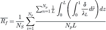$\bar{R_{f}} = \frac{1}{N_{S}} \sum_{i = 1}^{N_{p}} \frac{\sum_{n = 1}^{N_{p}} \frac{1}{L} \int_{0}^{L} (\int_{0}^{1} \frac{δ}{λ_{L}} d \tilde{r}) d z}{N_{p} L}$ $\bar{R_{f}} = \frac{1}{N_{S}} \sum_{i = 1}^{N_{p}} \frac{\sum_{n = 1}^{N_{p}} \frac{1}{L} \int_{0}^{L} (\int_{0}^{1} \frac{δ}{λ_{L}} d \tilde{r}) d z}{N_{p} L}$

(5.78)

where N_S, is the shell number in the heat exchanger for a multishell unit.

5.4.1.3. Hydraulics

The velocity inside the tubes, u, on which Re and, ultimately, the heat transfer coefficient and pressure drops depend, is written as a function of the flow area, A_flow (which is a function of the fouling thickness via Equation (5.69)):

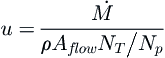$u = \frac{\dot{M}}{ρ A_{f l o w} N_{T} / N_{p}}$ $u = \frac{\dot{M}}{ρ A_{f l o w} N_{T} / N_{p}}$

(5.79)

where N_p denotes the number of tube-side passes and N_T the number of tubes in the heat exchanger. The definition of velocity as a function of the flow area allows to capture the effects of fouling growth on the hydraulic behavior of the exchanger. Quantities related to the velocity, such as the wall shear stress, τ, which governs the suppression term in Equation (5.77), are therefore also affected by fouling:

$τ = C_{f} (\frac{ρ u^{2}}{2})$ $τ = C_{f} (\frac{ρ u^{2}}{2})$

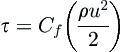(5.80)

where C_f is the Fanning friction factor for rough tubes (Yeap et al., 2004):

$C_{f} = 0.0035 + 0.264 R e^{- 0.42}$ $C_{f} = 0.0035 + 0.264 R e^{- 0.42}$

(5.81)

The physical properties appearing in the equations above are calculated using API relationships (Riazi, 2005) as a function of temperature and space. This allows to capture the effects of the variation in heat transfer coefficient along the length of the heat exchanger. Other thermophysical property models can be used if available.

5.4.2. Parameter Estimation Procedure

The model equations summarized above comprise a number of parameters. These can be divided in a set of two parameters:

• Set A, which includes the physical properties (i.e., °API, MeABP, and ν_100°F) of the fluids on both tube-side and shell-side. The values for these can, sometimes, be obtained from the refineries and may therefore be used as an input to the model rather than estimated.

• Set B, which includes the activation energy, E_f; preexponential deposition constant, A, and suppression constant, γ, in the fouling model, Equation (5.77). These quantities are not readily available and are difficult to measure experimentally.

The procedure developed by Coletti and Macchietto (2011) outlined below has been devised to use primary and readily available plant measurements (temperatures and flow rates) to estimate the necessary model parameters when these are not known:

1. Plant data are filtered according to a standardized procedure detailed in Coletti and Macchietto (2011) and summarized in Section 5.4.3. This procedures allow discarding from the estimation data set the data points that do not satisfy a minimum quality requirement.

2. The model is fitted by adjusting the values of the parameters to one set of plant data. A check is performed to assess whether it is able to reproduce those data.

3. The parameters obtained in step 2 are used to predict the outlet temperatures from the heat exchanger against a further set of plant data, different from the one used for the estimations. This step allows testing of the predictive capabilities of the model with the estimated value of the parameters.

Since parameters in Set A do not depend on fouling, they are estimated over the induction period when fouling has not yet started and the exchanger can be considered clean. This is defined as Period Ia or the “Clean period.” On the contrary, parameter set B should be estimated over a longer period where fouling is indeed affecting the performance of the unit. The latter is defined as Period I or the “Estimation period” and includes Period Ia. Mode-based parameter estimation techniques are used to estimate the values of the parameters that give the best fit to the retained plant data. The choice of Period Ia is important: it must start when the unit is fully cleaned and if too long, the assumption of no fouling being present on the tubes may not be valid. Conversely, if the period is too short, fluid properties may be fitted to a single oil slate, which may not be representative of the typical crudes processed by the refinery.

A second period immediately following Period I, Period II, defined as the ”Prediction period” is used to test the model for its predictive capabilities. The responses simulated using the parameter estimated in Period I are compared with plant measurements (outlet tube- and shell-side temperatures).

5.4.3. Plant Data

Raw plant measurements (rather than fouling resistances, derived from measurements with the use of simplistic heat balances) are used with model-based parameter estimation techniques to estimate values for the model parameters. This avoids incorporating in the analysis the errors resulting from any simplifying assumptions in calculations, such as the use of overall heat balances. Plant data are often considered unreliable by refinery operators. They typically trust temperature measurements to be within a ±5 °C error. However, for the parameter estimation procedure used here a variance of ±1 °C has been considered for all measurements as it will be justified later.

The measured outlet temperatures on both shell-side and tube-side are used to fit the model parameters in Period I following the procedure outlined above. These data are typically recorded at least on a daily basis, sometimes more frequently. Daily averages were used here. However, as highlighted by several authors (Crittenden et al., 1992) it is notoriously difficult to obtain reliable plant data, thus some judgment is required when analyzing such records.

As shown in Section 5.1, heat duties on both sides of the exchanger are typically calculated in refinery practice using a simple lumped heat balance model

$Q = \dot{M} c_{p} Δ T$ $Q = \dot{M} c_{p} Δ T$

(5.82)

that assumes constant mass flow rates, fluid physical properties, and heat transfer coefficients. Accuracy of the measurements is typically checked by calculating the percentage difference of the heat duty, Q, on the two sides of the heat exchanger. Here this difference is defined as the error φ:

$φ = \frac{Q_{S} - Q_{T}}{Q_{S}} %$ $φ = \frac{Q_{S} - Q_{T}}{Q_{S}} %$

(5.83)

where Q_S is the heat duty on calculated on the shell-side and Q_T is the heat duty calculated on the tube-side. Given the many assumptions described above, values of the error φ = 10–30% are often found when using raw plant measurements. Moreover, such errors typically have a significant nonzero average offset and wide variability (Crittenden et al., 1992).

Rigorous statistical methodologies existing in the literature could be used to detect instrument bias prior to the use of the following procedure. However, it is assumed here that the measurements do not suffer from systematic bias for the time periods considered and thus a simple procedure is sufficient to screen out grossly inaccurate measurements that would otherwise cause numerical problems in the estimation of model parameters and result in wrong parameter values. The procedure proposed by Coletti and Macchietto (2011) calculates φ from Equation (5.83) using measured plant temperature and flow rate data, and estimates its average over time

\bar{φ}

$\bar{φ}$

and standard deviation σ. Daily data for which φ deviates more than a certain value from the mean are deemed to be grossly erroneous or outliers and are discarded from consideration for parameter fitting purposes. The remaining data are defined as filtered and are used in a proper statistically sound model-based parameter estimation, in conjunction with the full detailed dynamic model, using the procedure described in Section 5.4.2.

5.4.4. Implementation

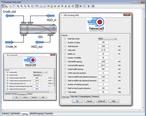
One key characteristic of a good tool is its user friendliness. As shown in Figure 5.39 the setup of a single heat exchanger model is performed via a tailored interface through specially designed interactive forms and drag-and-drop items. Key attributes to be specified include oil characteristics, heat exchanger characteristics, and parameters for fouling and aging. A standardized interface with Excel is also available for importing exchanger geometry data directly from refinery proprietary data sheets. Once specified, each particular exchanger may be added to the general Hexxcell Studio™ library. Individual library components may be reused alone or assembled in combination with other models to provide higher level models. The framework then allows a rapid replication of similar units and interconnecting them together, via simple drag-and-drop, to construct a heat exchanger network model (Figure 5.40). This allows to quickly match a current preheat train configuration, or alternative ones being assessed. The composite network model (e.g., an entire preheat train or a section of it) may itself be saved in the Hexxcell Studio™ library and reused, alone or with other models. This way, it is very easy to generate alternative configurations at various levels of aggregation, test and evaluate modifications under exactly the same conditions, etc. The cost parameters of an economic model (e.g., pumping costs, furnace fuel costs, production loss) may also be defined, to help assess performance in economic rather than purely technical terms.

Figure 5.39 Specification of a shell-and-tube heat exchanger and fouling model parameters. Copyright (2014) Hexxcell Ltd.

Although the number of equations in the model is fairly large when an entire preheat network is simulated, it is possible to obtain a solution in a few minutes of computational time. It typically takes less than ca. 300 s to an Intel i7 processor at 3.4 GHz with 8 GB RAM to solve a 10 heat exchanger network. Moreover, the robustness of the model is ensured by the use of Hexxcell's proprietary initialization procedures which allow the solver to determine the initial point for the calculations transparently to the user. As a result, the model can be easily initialized and used by thermal and process engineers at all levels without the support of a specialist in numerical techniques.

5.4.5. Model Validation and Results for Individual Heat Exchangers

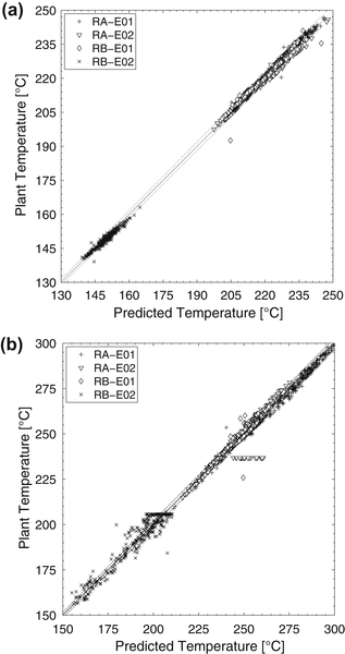
The details of the model validation are reported in Coletti and Macchietto (2010b, 2011). To show the model validation over a wide range of operating conditions a short summary is given here based on the results reported by Coletti and Macchietto (2010b) for four industrial units in two refineries operated by major oil companies:

• RA-E01, RA-E02. Two double shell units in Refinery A.

• RB-E01, RB-E02. Two single shell units in Refinery B.

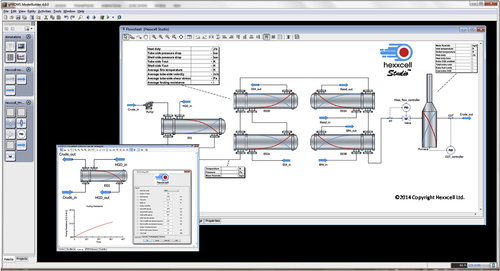
Figure 5.40 Screenshot of the graphical user interface of a preheat train model using the Hexxcell Studio™ library. Copyright (2014) Hexxcell Ltd.

Table 5.12

Summary of data used. Reproduced with permission from Coletti and Macchietto (2010b).

HEX name	N_s	N_p	T_s [°C]	T_t [°C]	Design u_t [m s⁻¹]	Run length [d]
RA-E01	2	4	220–350	190–250	2.5	349
RA-E02	2	4	220–320	170–250	1	162
RB-E01	1	4	240–300	180–210	1.7	550
RB-E02	1	2	155–270	130–160	2.7	310

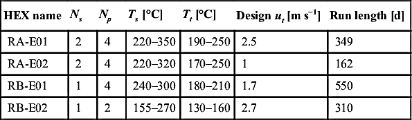
Temperature range refers to the minimum coldest and the maximum hottest temperature on record for a given side of the unit. Run length is the period of time between two mechanical cleanings considered for the analysis.

The use of data from different refineries is particularly important to ensure that the model capabilities in predicting fouling behavior are not refinery specific or oil specific. While refineries typically change crude blends every 2–3 days, the crude types processed by one refinery are usually from a limited number of geographic origins. As a result, testing the model on data from different refineries has the significance of generalizing its validity to a large number of crude blends. Moreover, considering units from different refineries also means dealing with different design and operating philosophies. The geometries considered vary with respect to shell size, number of tube passes, tube diameter, pitch angle, baffle number, spacing, etc. The range of operating temperatures considered is 150–350 °C on the shell-side and 130–245 °C on the tube-side (Table 5.12).

In particular, one of the units, RB-E02, operated at a relatively low temperature (crude is between c. 130 and 150 °C) just below the range in which chemical reaction fouling is believed to be the dominant fouling mechanism. The hydraulic conditions on the tube-side considered also vary significantly. The design velocity of the heat exchanger considered ranges between 1 and 2.5 m s⁻¹.

For all the units considered, Period Ia was set to include the first 15 accurate measurements. Depending on the quality of the data, φ, it ends at different dates for each unit. Period I was 60 days for all units. The length of the prediction period, Period II, is related to the length of the run specific for each exchanger, which is between 162 and 550 days (last column of Table 5.12). The prediction periods considered here therefore range from 5.5 months for unit RA-E2 in this study up to 16 months for unit RB-E01.

The procedure used for parameter estimation and results of the model predictions are illustrated in the following section in detail for exchanger RA-E01; the results for other cases are reported in Section 3.4.5.2. Section 5.4.6.2 shows how the model can be used to propose effective retrofits that minimize fouling and maximize energy efficiency.

5.4.5.1. Model Results and Predictions for RA-E01

The heat exchanger considered comprised two identical shells with four tube passes per shell. The crude was allocated on the tube-side, whereas residuum from the crude distillation column was on the shell-side. Refinery observation when dismantling the unit for cleaning indicated that, although some shell-side fouling was detected, the dominant fouling resistance was on the tube-side.

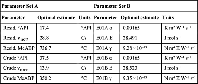
Parameters in Set A and Set B were estimated over Period I using plant data (inlet temperatures and volumetric flow rates) starting after a mechanical cleaning. Over this period, 30% of the data points were discarded as deemed inaccurate by the procedure described above. The estimated parameters are reported in Table 5.13.

To test whether the model can be used in a predictive mode (i.e., to extrapolate its results beyond the estimation period, without reestimating its parameters), the model was then used to simulate the exchanger for the rest of the year. Measured inlet temperatures and flow rates were input to the simulation, but all adjustable parameters were kept fixed. The simulated performance, in terms of output temperatures over the whole time horizon considered (347 days) is shown by the continuous lines in Figures 5.41 and 5.42, together with plant measurements. The exit temperatures on both sides were predicted well over the entire period, even in the presence of rather major excursions, including the period between 60–100 days.

The contribution of fouling and aging to the overall behavior of the unit is illustrated by the two extra lines plotted in the same figures:

1. The dashed line was obtained using the same parameter Set A as before but setting the fouling rate to 0 (i.e., dR_f/dt = 0), corresponding to a case in which fouling had not occurred and the heat exchanger operated in clean conditions.

Table 5.13

Estimates for parameter Set A and B. Parameter Set B shows estimates of the fouling model in each shell comprising the heat exchanger. Reproduced with permission from Coletti and Macchietto (2011).

Parameter Set A			Parameter Set B
Parameter	Optimal estimate	Units	Parameter	Optimal estimate	Units
Resid. °API	17.4	°API	E01A α	0.00165	K m² W⁻¹ s⁻¹
Resid. ν_100°F	28.8	Cs	E01A E	28,491	J mol s⁻¹
Resid. MeABP	736.7	°C	E01A γ	9.28 × 10⁻¹³	N m⁴ K W⁻¹ s⁻¹
Crude °API	37.5	°API	E01B α	0.00165	K m² W⁻¹ s⁻¹
Crude ν_100°F	13.9	Cs	E01B E	28,523	J mol s⁻¹
Crude MeABP	350.2	°C	E01B γ	9.35 × 10⁻¹³	N m⁴ K W⁻¹ s⁻¹

Figure 5.41 Overlay plot over the 350 days after cleaning of model simulations with tube-side outlet temperature. Dashed line shows simulation run setting R_f = 0 whereas the dashed–dotted line shows simulation results with no aging. White markers show data filtered with the procedure developed whereas colored markers show data deemed inaccurate. The error bars indicate ±1 °C. The vertical dashed line shows the end of Period Ia whereas the dotted line indicates the end of Period I and the beginning of Period II. Reproduced with permission from Coletti and Macchietto, A dynamic, distributed model of shell-and-tube heat exchangers undergoing crude oil fouling, 2011. Ind. Eng. Chem. Res. 50(8): 4515–4533. Copyright (2011) American Chemical Society.

Figure 5.42 Overlay plot over the 350 days after cleaning of model simulations with shell-side outlet temperature. Dashed line shows simulation run setting R_f = 0 whereas the dashed-dotted line shows simulation results with no aging. White markers show data filtered with the procedure developed whereas colored markers show data deemed inaccurate. The error bars indicate ±1 °C. The vertical dashed line shows the end of Period Ia whereas the dotted line indicates the end of Period I and the beginning of Period II. Reproduced with permission from Coletti and Macchietto, A dynamic, distributed model of shell-and-tube heat exchangers undergoing crude oil fouling, 2011. Ind. Eng. Chem. Res. 50(8): 4515–4533. Copyright (2011) American Chemical Society.

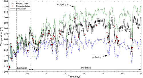
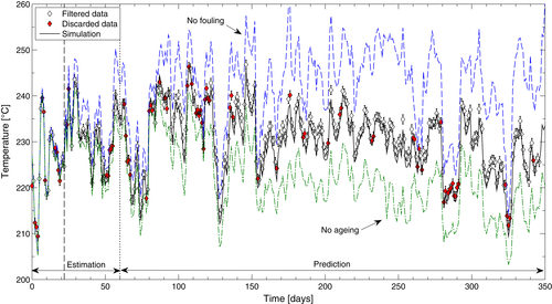
2. The dashed–dotted line was obtained using same parameter Sets A and B but setting the preexponential term in the aging model to 0, corresponding to a case in which fouling occurred but the deposits did not age.

Figures 5.41 and 5.42 provide an insight on the opposite effects of fouling and aging on the crude outlet temperature. Whilst fouling reduced the heat transfer efficiency thus decreasing the crude outlet temperature of the heat exchanger, aging acted in the opposite way, by increasing the thermal conductivity of the deposits, thus enhancing the overall heat transfer. Temperature estimated without fouling or aging in the model did not match the plant data, but did so when both phenomena were included.

The contribution of each of the two shells, E01A and E01B to the overall average fouling resistance

\bar{R_{f}}

$\bar{R_{f}}$

, calculated from Equation (5.78), is shown in Figure 5.43. As expected for a clean exchanger, the value of the fouling resistance increased from an initial zero value. The rate of increase was high initially but reduced after about 150 days to an approximately constant value. Fouling in shell E01A was slightly higher than in shell E01B but the difference (in this case) was not large. Model outputs for

\bar{R_{f}}

$\bar{R_{f}}$

were also compared with refinery calculations. The latter showd a zero fouling resistance for the first few days, after which a sharp jump to an offset value of ca. 2 × 10⁻³ m²KW⁻¹ occurd.

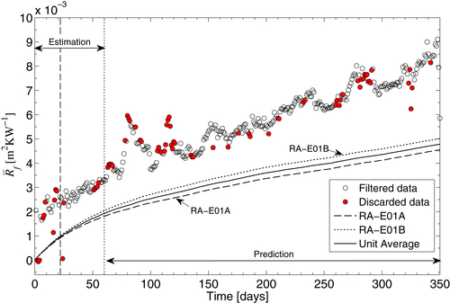
Figure 5.43 Refinery-calculated fouling resistance and model-calculated overall average R_f. The dotted and dashed lines indicate average R_f calculated for RA-E01A and RA-E01B respectively. Reproduced with permission from Coletti and Macchietto, A dynamic, distributed model of shell-and-tube heat exchangers undergoing crude oil fouling, 2011. Ind. Eng. Chem. Res. 50(8): 4515–4533. Copyright (2011) American Chemical Society.

Given the high degree of accuracy of the exit temperatures predicted by the model, it is likely that the overall fouling resistance calculated by the refinery merely reflects the gross approximations (e.g., in physical properties) used in its calculation. The overall trends shown substantially agree, and when the offset is subtracted, numerical values are also close. In particular, Figure 5.43 shows that the (perceived) sudden increase in fouling resistance around 80–100 days can be fully explained by the measured changes in inlet flow rates, temperatures, and complex interactions arising.

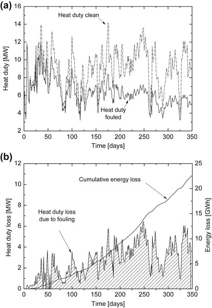
One of the main benefits of the model is that it enables the identification of the effects of fouling on the performance of the heat exchanger. Figure 5.44(a) reports the heat duty from model simulations in the case of fouling and no fouling over time for the heat exchanger RA-E01. It can be noted that the two curves diverge significantly over time. The difference between the two heat duties shown in Figure 5.44(b) represents the energy lost instantly due to fouling. Figure 5.44(b) also shows the integral of the heat duty loss over time, which represents the cumulative energy loss, calculated as 22.4 GWh after 347 days of operations. If this loss were to be compensated entirely at the furnace (i.e., no dumping effects given by the interaction with other exchangers in the network), the cost in extra fuel burnt would be in excess of US$670,000 (based on fuel a cost of US$27 MWh^-1 and 90% efficiency of the furnace).

5.4.5.2. Model Results and Predictions for Other Heat Exchangers

To test the range of applicability of the model in a variety of cases, the same procedure described for RA-E01 was applied to the other three heat exchangers in Table 5.12.

The residuals (Figure 5.45) for each individual heat exchanger show some weak systematic trend, as opposed to purely random scatter, indicating there is possibly some underlying model mismatch (not surprising, for example, in view of the many oil slate changes over the long periods of time considered). Even so, 93% of all data are within ±2% error on the shell-side (ca. ±4 °C) and ±1% on the tube-side (ca. ±2 °C). The major deviation is given by RB-E02, which is expected as this is the lowest temperature unit and small absolute errors translate into large percentage errors. It should be noted that the values of the residuals calculated also depend on the temperature scale used.

Figure 5.44 Heat duty from model simulations in case of fouling and no fouling over time in unit RA-E01 (a). The energy lost due to fouling, represented by the shaded area, and the cumulative energy loss over time are given in (b).

It is interesting to note that the quality of model predictions remained good (within a narrow error band) over extended periods of time (up to 16 months). These are industrially relevant time horizons as required for planning of cleanings to optimize a refinery economic performance.

Figure 5.46 reports parity plots of the predicted versus measured temperatures for the shell (a) and tube (b) sides, for all four units, thus covering a wide temperature range. The dashed lines show a deviation of ±1% from the parity line. Analysis of these plots reveals that over 80% of the points are within a ±1% error for both sides of the unit. It should be noted that this 80% includes points which are given by clearly erroneous measurements (e.g., the previously noted flat plant temperatures at ca. 235 °C, evident in Figure 5.46(a)). This analysis provides an a posteriori justification of the use of ±1 °C variance in the measurements, which was used in the parameter estimation step.

Figure 5.45 Percentage residuals between plant measurements of fluid outlet temperatures (in °C) and model simulations on the shell (a) and tube (b) side for all units examined. The vertical, dashed line indicates the end of the estimation period (Period I) and the horizontal dashed line indicates zero error. Reproduced with permission from Coletti and Macchietto, Validation of a novel model for Shell–and–Tube heat exchangers undergoing crude oil fouling, 2010. In: Proc. 14^th Int. Heat Transfer Conf. (IHTC14); Vol. 4, Washington, DC, USA, August 8–13. ASME, pp. 741–750. Copyright (2010) ASME.

Figure 5.46 Parity plot of fluid outlet temperature on the shell (a) and tube (b) side for all units examined. The dashed lines indicate ±1% deviation from the parity line on the diagonal. Reproduced with permission from Coletti and Macchietto, Validation of a novel model for Shell–and–Tube heat exchangers undergoing crude oil fouling, 2010. In: Proc. 14^th Int. Heat Transfer Conf. (IHTC14); Vol. 4, Washington, DC, USA, August 8–13. ASME, pp. 741–750. Copyright (2010) ASME.

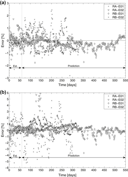
The estimated fouling activation energy, E_f, shows a remarkable consistency, varying between 28.5 and 32.1 kJ mol⁻¹ and compares well with typical values reported in the literature for crude oil reaction fouling.

5.4.5.3. Retrofit of Unit RA-E01

The model validation with plant data performed in the previous section gives the necessary confidence to exploit its capabilities to assess alternative design that might mitigate fouling and reduce energy losses. The detailed analysis carried out in the previous section unveiled that energy losses produced by fouling in unit RA-E01 added up to 22.4 GWh after 347 days of operation. In this section, a study of a simple retrofit option which aimed at reducing these losses is reported.

It has already been noted in previous Chapters of this book that increasing velocity—thus wall shear stress—has a beneficial effect on fouling and it is the process variable on which the designer has most control. It seems reasonable therefore to choose this variable first to improve the unit's performance. For a given flow rate, a way of achieving higher velocities within the tubes is to increase the number of tube-side passes, N_p. This is a relatively inexpensive option to be implemented in existing units as it requires only replacement of the heat exchanger headers, leaving in place existing tube bundle and shell.

In the case considered here, the retrofit of unit RA-E01 was performed by increasing the number of tube-side passes of the existing configuration from 4 to 6. All other geometric parameters (e.g., flow arrangement, number of tubes) were kept at the original values. Values of physical properties and the fouling model parameters were fixed at the values estimated with the procedure described in Section 5.4. Simulations were then performed under the same plant conditions, over 347 days after a mechanical cleaning, used for the 4 pass unit. This allowed for testing how the retrofitted unit would have performed in the refinery if the proposed design were actually used under the process conditions experienced in the plant. Comparison with simulation results reported in the previous section for the existing exchanger allows assessment of the potential saving achievable with the new configuration.

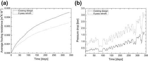
Figure 5.47(a) shows the reduction in fouling resistance produced by the higher velocities within the 6 pass exchanger. The value of the overall fouling resistance was reduced by ca. 25% after a year of operations, at the expenses of an increased pumping power required to counter the larger pressure drop (Figure 5.47(b)). While the extra pressure drop generated by the new configuration, ca. 0.5 bar, seemed acceptable under clean conditions, at the end of the operating period, it reached ca. 3 bar. This may be accepted, depending on the hydraulic flexibility of the refinery (considerations on mechanical design are excluded in this preliminary analysis).

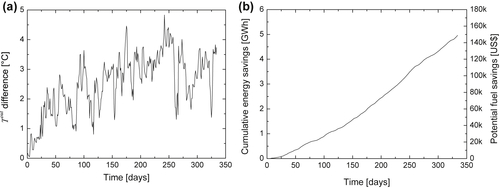
Figure 5.48(a) shows that the difference in outlet temperatures of the tube-side fluid (crude) between operations with the existing unit and the retrofitted one was as large as 4 °C. Cumulative energy savings were estimated to add up to almost 5 GWh (Figure 5.48(b)). This is equivalent to a 22% reduction in the heat duty losse generated by fouling in the first 347 days of operation and to ca. US$150,000 savings in furnace fuel alone.

Figure 5.47 Fouling resistance (a) and pressure drops (b) in the existing design compared with the retrofit configuration proposed. Pressure drop values shown do not include headers and nozzles.

Figure 5.48 Difference in tube-side outlet temperature between the existing and the retrofitted unit (a) and cumulative energy savings, with respect to the existing unit, achieved using the 6 pass design (b) under the plant operating conditions.

5.4.6. Whole Preheat Train Case Study

The detailed dynamic model described above is for a single shell-and-tube heat exchanger. However, in a PHT, no heat exchanger exists on its own and the distinct fouling behavior of each heat exchanger affects the overall performance of the network. Complex interactions among the heat exchangers can only be unveiled by a simulation of the entire network. The implementation of the model equations as detailed in Section 5.4.4 greatly facilitates the setup of a network simulation. All the necessary equations that govern the single heat exchanger model are wrapped in an object that can be easily instantiated through a graphic user interface and readily replicated in a flowsheet environment to generate the topology of a specific network.

The operation of the network is simulated via the simultaneous solution of equations for all exchangers. Each exchanger in the network is represented using the detailed dynamic model with suitably instantiated parameters for geometry, fouling, aging, etc. Simulating each unit at this level of detail allows gaining insights on how each heat exchanger individually contributes to the overall network performance.

5.4.6.1. Assessment of Network Performance: Key Performance Indicators

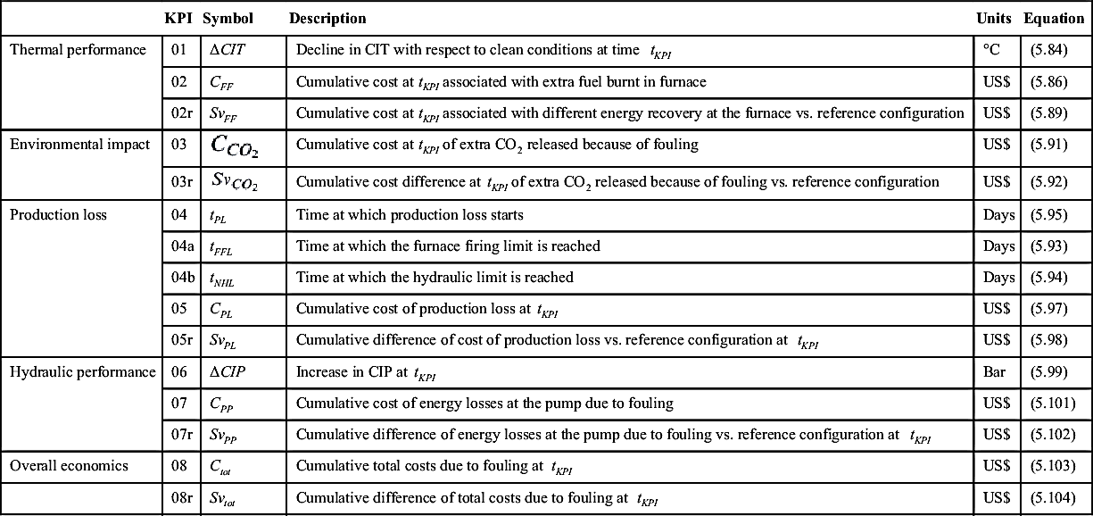
Variable flow conditions, temperatures, and crude slates as well as geometry of single HEXs and structure of the network affect different ways of the fouling behavior of a PHT, thus the energy recovered and, ultimately, the refinery bottom line. However, given the large number of variables involved, it may be difficult to isolate causes of inefficiencies and identify different variables contributing to the overall performance. The task of identifying dynamic interactions among units is particularly challenging when considering different structures for network retrofit. To assess in a consistent way the performance of a PHT network undergoing fouling and to be able to evaluate potential benefits in restructuring the network, the set of key performance indicators proposed by Coletti et al. (2011) is summarized in the following section with a modification introduced to also take into account possible hydraulic limitations of the heat exchanger network. In what follows, each network structure is denoted by Cj where j is the number of the configuration considered.

Given that the phenomena involved are intrinsically dynamic, some of the KPIs presented in the following sections (and summarized in Table 5.14) are referred to a reference time, t_KPI, and used to provide a snapshot of network conditions and history up to that point in time. Some of these indicators refer to clean conditions which can be easily calculated at time 0 if all the heat exchangers in the network can be assumed clean at that time and the inputs (flow rate, temperature, and pressure) are kept constant. However, if real plant data are to be used as input, it is not easy to determine a reference clean conditions performance. In this case model simulations can be exploited to provide reference clean conditions by setting R_f = 0 in each heat exchanger.

5.4.6.1.1. Fuel Costs

The decline in CIT with respect to clean conditions over time for any network j can be used as a measure of the overall thermal performance of the network:

$Δ C I T = C I T_{c l e a n} - C I T$ $Δ C I T = C I T_{c l e a n} - C I T$

(5.84)

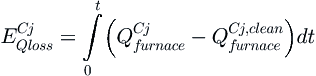
Equation (5.84) evaluated at t = t_KPI provides KPI-01, the first key performance indicator considered here. The energy loss associated with the extra fuel burnt at the furnace to compensate the decrease in CIT,

E_{Q l o s s}^{C j}

$E_{Q l o s s}^{C j}$

, is calculated as the integral over time of the difference between the total actual heat supplied by the furnace to the crude,

Q_{f u r n a c e}^{C j}

$Q_{f u r n a c e}^{C j}$

, and the total heat duty under clean conditions,

Q_{f u r n a c e}^{C j, c l e a n}

$Q_{f u r n a c e}^{C j, c l e a n}$

$E_{Q l o s s}^{C j} = \int_{0}^{t} (Q_{f u r n a c e}^{C j} - Q_{f u r n a c e}^{C j, c l e a n}) d t$ $E_{Q l o s s}^{C j} = \int_{0}^{t} (Q_{f u r n a c e}^{C j} - Q_{f u r n a c e}^{C j, c l e a n}) d t$

(5.85)

Taking into account overall efficiency of the furnace, η_furnace, the cost of this extra energy requirement is a function of the cost of the fuel being burnt, P_fuel:

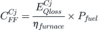$C_{F F}^{C j} = \frac{E_{Q l o s s}^{C j}}{η_{f u r n a c e}} \times P_{f u e l}$ $C_{F F}^{C j} = \frac{E_{Q l o s s}^{C j}}{η_{f u r n a c e}} \times P_{f u e l}$

(5.86)

C_{F F}^{C j}

$C_{F F}^{C j}$

evaluated at time t = t_KPI provides KPI-02. To evaluate different retrofit options, it is useful to compare this cost for given network structure, configuration Cj, with that in a reference configuration, C1. To do this, first it is necessary to calculate the total (cumulative) energy required for each configuration considered:

Table 5.14

Summary of key performance indicators (KPI) for assessment of network performance

	KPI	Symbol	Description	Units	Equation
Thermal performance	01	ΔCIT	Decline in CIT with respect to clean conditions at time t_KPI	°C	(5.84)
	02	C_FF	Cumulative cost at t_KPI associated with extra fuel burnt in furnace	US$	(5.86)
	02r	Sv_FF	Cumulative cost at t_KPI associated with different energy recovery at the furnace vs. reference configuration	US$	(5.89)
Environmental impact	03	$C_{C O_{2}}$ $C_{C O_{2}}$	Cumulative cost at t_KPI of extra CO₂ released because of fouling	US$	(5.91)
Environmental impact	03r	$S v_{C O_{2}}$ $S v_{C O_{2}}$	Cumulative cost difference at t_KPI of extra CO₂ released because of fouling vs. reference configuration	US$	(5.92)
Production loss	04	t_PL	Time at which production loss starts	Days	(5.95)
	04a	t_FFL	Time at which the furnace firing limit is reached	Days	(5.93)
	04b	t_NHL	Time at which the hydraulic limit is reached	Days	(5.94)
	05	C_PL	Cumulative cost of production loss at t_KPI	US$	(5.97)
	05r	Sv_PL	Cumulative difference of cost of production loss vs. reference configuration at t_KPI	US$	(5.98)
Hydraulic performance	06	ΔCIP	Increase in CIP at t_KPI	Bar	(5.99)
	07	C_PP	Cumulative cost of energy losses at the pump due to fouling	US$	(5.101)
	07r	Sv_PP	Cumulative difference of energy losses at the pump due to fouling vs. reference configuration at t_KPI	US$	(5.102)
Overall economics	08	C_tot	Cumulative total costs due to fouling at t_KPI	US$	(5.103)
	08r	Sv_tot	Cumulative difference of total costs due to fouling at t_KPI	US$	(5.104)

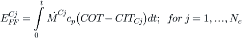$E_{F F}^{C j} = \int_{0}^{t} {\dot{M}}^{C j} c_{p} (C O T - C I T_{C j}) d t; f o r j = 1, \dots, N_{c}$ $E_{F F}^{C j} = \int_{0}^{t} {\dot{M}}^{C j} c_{p} (C O T - C I T_{C j}) d t; f o r j = 1, \dots, N_{c}$

(5.87)

where N_c denotes the number of retrofit configurations explored and CIT_j is the coil inlet temperature in each configuration j, and COT the fixed coil outlet temperature, required for distillation. The difference in performance (extra energy recovered at the furnace) of each retrofit provides the comparison between the different configurations considered:

$Δ E_{F F}^{C 1 - C j} = E_{F F}^{C 1} - E_{F F}^{C j}; f o r j = 1, \dots, N_{c}$ $Δ E_{F F}^{C 1 - C j} = E_{F F}^{C 1} - E_{F F}^{C j}; f o r j = 1, \dots, N_{c}$

(5.88)

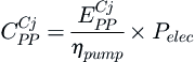
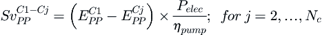
In economic terms, the furnace fuel savings of a particular configuration Cj with respect to C1,

S v_{F F}^{C 1 - C j}

$S v_{F F}^{C 1 - C j}$

, associated with

Δ E_{F F}^{C 1 - C j}

$Δ E_{F F}^{C 1 - C j}$

are

$S v_{F F}^{C 1 - C j} = \frac{Δ E_{F F}^{C 1 - C j}}{η_{f u r n a c e}} P_{f u e l}; f o r j = 1, \dots, N_{c}$ $S v_{F F}^{C 1 - C j} = \frac{Δ E_{F F}^{C 1 - C j}}{η_{f u r n a c e}} P_{f u e l}; f o r j = 1, \dots, N_{c}$

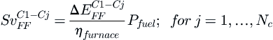(5.89)

The cumulative fuel savings up to time t = t_KPI provide the KPI-02r indicator for network retrofit.

5.4.6.1.2. Emission Costs

The combustion of extra fuel produces the release of greenhouse gases to the environment, which, under environmental laws (e.g., the Emissions Trading Scheme in Europe), adds economic penalties to the operations. In this study it is assumed that under clean conditions the refinery is just within its allocated allowance and that any extra ton of carbon dioxide caused by fouling,

M_{C O_{2}}^{C j}

$M_{C O_{2}}^{C j}$

, must be paid for:

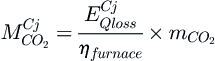$M_{C O_{2}}^{C j} = \frac{E_{Q l o s s}^{C j}}{η_{f u r n a c e}} \times m_{C O_{2}}$ $M_{C O_{2}}^{C j} = \frac{E_{Q l o s s}^{C j}}{η_{f u r n a c e}} \times m_{C O_{2}}$

(5.90)

In Equation (5.90),

m_{C O_{2}}

$m_{C O_{2}}$

denotes the carbon emission per Joule of energy produced in the combustion of a given fuel.

$C_{C O_{2}}^{C j} = M_{C O_{2}}^{C j} \times P_{C O_{2}}$ $C_{C O_{2}}^{C j} = M_{C O_{2}}^{C j} \times P_{C O_{2}}$

(5.91)

where

P_{C O_{2}}

$P_{C O_{2}}$

is the price per ton of CO₂.

C_{C O_{2}}^{C j}

$C_{C O_{2}}^{C j}$

at t = t_KPI provides KPI-03 for configuration Cj. If network retrofit is considered, the savings in CO₂ emissions for each configuration Cj with respect to the reference configuration C1 are calculated from the fuel energy savings in Equation (5.92):

$S v_{C O_{2}}^{C 1 - C j} = Δ E_{F F}^{C 1 - C j} \times \frac{m_{C O_{2}}}{η_{f u r n a c e}} \times P_{C O 2}; f o r j = 2, \dots, N_{c}$ $S v_{C O_{2}}^{C 1 - C j} = Δ E_{F F}^{C 1 - C j} \times \frac{m_{C O_{2}}}{η_{f u r n a c e}} \times P_{C O 2}; f o r j = 2, \dots, N_{c}$

(5.92)

The cumulative CO₂ savings up to time t = t_KPI provide the KPI-03r for network retrofit.

5.4.6.1.3. Production Loss

As noted in Chapter 1, the reduction in thermal and hydraulic efficiency caused by fouling is paid not only at the furnace or the pump as extra energy but also as loss of production. When the furnace hits its firing limit, the throughput must be reduced causing a cost in loss of production. The time when this happens, t_FFL, provides a key performance indicator KPI-04a:

$t_{F F L} = {t |}_{Q = Q^{m a x}}$ $t_{F F L} = {t |}_{Q = Q^{m a x}}$

(5.93)

If the pressure drop across the preheat train reaches a maximum value beyond which any increase cannot be compensated for by the hydraulic systems, the hydraulic limit of the network is reached. The time at which this happens is KPI-04b

$t_{N H L} = {t |}_{Δ P = Δ P^{m a x}}$ $t_{N H L} = {t |}_{Δ P = Δ P^{m a x}}$

(5.94)

Whether the thermal or the hydraulic limit is reached, the result is that production needs to be reduced:

$t_{P L} = m i n (t_{F F L}, t_{N H L})$ $t_{P L} = m i n (t_{F F L}, t_{N H L})$

(5.95)

The production loss, M_PL, associated with the reduction in throughput due to either the thermal or the hydraulic limit is

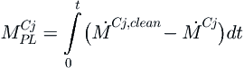$M_{P L}^{C j} = \int_{0}^{t} ({\dot{M}}^{C j, c l e a n} - {\dot{M}}^{C j}) d t$ $M_{P L}^{C j} = \int_{0}^{t} ({\dot{M}}^{C j, c l e a n} - {\dot{M}}^{C j}) d t$

(5.96)

where

{\dot{M}}_{c l e a n}

${\dot{M}}_{c l e a n}$

is the mass flow rate under clean conditions and

\dot{M}

$\dot{M}$

is the actual throughput. The cost associated with the production loss,

C_{PL}^{C j}

$C_{PL}^{C j}$

, is then calculated as

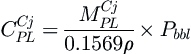$C_{P L}^{C j} = \frac{M_{P L}^{C j}}{0.1569 ρ} \times P_{b b l}$ $C_{P L}^{C j} = \frac{M_{P L}^{C j}}{0.1569 ρ} \times P_{b b l}$

(5.97)

where P_bbl is the operating margin per barrel of crude, ρ the crude density, and 0.1569 is a conversion factor.

C_{PL}^{C j}

$C_{PL}^{C j}$

as calculated in Equation. (5.97) at time t = t_KPI provides KPI-05.

To assess network retrofit performance with respect to production loss, the difference (excess) in production achieved by each configuration Cj with respect to the reference configuration C1 is calculated from the difference in mass flow rate over time. The associated production loss savings are

$S v_{P L}^{C 1 - C j} = C_{P L}^{C 1} - C_{P L}^{C j}; f o r j = 2, \dots, N_{c}$ $S v_{P L}^{C 1 - C j} = C_{P L}^{C 1} - C_{P L}^{C j}; f o r j = 2, \dots, N_{c}$

(5.98)

S v_{P L}^{C 1 - C j}

$S v_{P L}^{C 1 - C j}$

evaluated at t = t_KPI denotes KPI-05r.

5.4.6.1.4. Assessment of Hydraulic Efficiency

The reduction in cross-sectional area inside the heat exchanger tubes produces an increase in pressure drops that must be countered by increasing the energy supplied to the pump to maintain the largest throughput achievable within the furnace firing limit constraint. Pressure drops, shear stress, and velocity within individual heat exchangers can be used to evaluate the hydraulic impact of fouling. However, the hydraulic performance of the whole network can be assessed via the increase in coil inlet pressure (CIP) over time with respect to clean conditions:

$Δ C I P = C I P_{c l e a n} - C I P$ $Δ C I P = C I P_{c l e a n} - C I P$

(5.99)

The value of ΔCIP at t = t_KPI provides KPI-06. The cost of energy loss associated with the increase in pumping power required to counter the hydraulic effects of fouling is another useful indicator of the network performance. The integral over time of the difference between pumping power under clean conditions, W_clean, and the actual pumping power (i.e., under fouled conditions), W, gives the energy losses at the pump due to fouling,

E_{P P}^{C j}

$E_{P P}^{C j}$

$E_{P P}^{C j} = \int_{0}^{t} (W^{C j} - W^{C j, c l e a n}) d t$ $E_{P P}^{C j} = \int_{0}^{t} (W^{C j} - W^{C j, c l e a n}) d t$

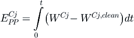(5.100)

This translates in extra electricity costs due to fouling-related extra pumping power requirements as

$C_{P P}^{C j} = \frac{E_{P P}^{C j}}{η_{p u m p}} \times P_{e l e c}$ $C_{P P}^{C j} = \frac{E_{P P}^{C j}}{η_{p u m p}} \times P_{e l e c}$

(5.101)

where P_elec denotes the price of electricity, η_pump denotes the pump efficiency.

C_{P P}^{C j}

$C_{P P}^{C j}$

evaluated at t = t_KPI provides KPI-07. In the case of a retrofit, the CIP in a given configuration C1 is compared to that in a reference configuration C1. The savings in pumping power can be estimated from the total (cumulative) pumping power required for each configuration Cj, and the price of electricity:

$S v_{P P}^{C 1 - C j} = (E_{P P}^{C 1} - E_{P P}^{C j}) \times \frac{P_{e l e c}}{η_{p u m p}}; f o r j = 2, \dots, N_{c}$ $S v_{P P}^{C 1 - C j} = (E_{P P}^{C 1} - E_{P P}^{C j}) \times \frac{P_{e l e c}}{η_{p u m p}}; f o r j = 2, \dots, N_{c}$

(5.102)

which, calculated at t = t_KPI, indicates KPI-07r for network retrofit.

5.4.6.1.5. Overall Fouling Costs

The cumulative cost of fouling, C_tot, evaluated at t = t_KPI denotes KPI-08 which comprehensively summarizes the economic impact of fouling in the CDU.

Starting at time 0 from clean conditions for the PHT, the extra costs due to fouling for a given network Cj are evaluated as:

$C_{t o t} = C_{F F} + C_{C O_{2}} + C_{P L} + C_{P P}$ $C_{t o t} = C_{F F} + C_{C O_{2}} + C_{P L} + C_{P P}$

(5.103)

where C_FF is the cost of the additional fuel that must be burnt in the furnace to counter the decline over time in the oil temperature at its inlet, the coil inlet temperature (CIT), C_PL is the cost associated with the reduction in throughput,

C_{C O_{2}}

$C_{C O_{2}}$

is the costs associated with the extra emission of CO₂ due to fouling, and C_PP is the electricity cost due to increase in pumping power required to maintain a constant throughput.

For network retrofit, KPI-08r is the sum of KPI-02r, KPI-03r, KPI-05r, and KPI-07r:

$S v_{t o t}^{C 1 - C j} = C_{t o t}^{C 1} - C_{t o t}^{C j}$ $S v_{t o t}^{C 1 - C j} = C_{t o t}^{C 1} - C_{t o t}^{C j}$

(5.104)

Cleaning and shutdown costs are not considered here. The assessment of the costs is therefore based on no action having been taken to clean any unit. The following sections detail the calculations for the each of the terms in Equation (5.103).

5.4.6.2. Case Study on Entire Preheat Train

Coletti et al. (2011) showed that using high-fidelity thermo-hydraulic simulations to capture complex dynamic interactions in the network provides a more useful way to analyze alternative PHT retrofit options than currently available. For this purpose, a network was modeled based on an industrial case study of a small refinery (ca. 20,000 bbl day⁻¹). In order to protect proprietary information, the heat and mass balance for the existing network comprising seven exchangers were adjusted and some features of the plant were changed without affecting the validity of the conclusions. This network structure represented the base case for the study and was referred to as configuration C1 (Figure 5.49). The performance of the preheat train was monitored at startup (after cleaning) and after 8000 h of operation. While units E-01, E-02, and E-04 did not change significantly their performance over the operating period, the other four units in the network exhibited severe fouling. The observations of the refinery operators were that fouling in units E-05 and E-06 occurred mainly on the tube-side (were crude oil was allocated) and this was the only side of these units which was Periodically cleaned. Unit E-03 fouled on the shell-side (which handled column residues) but not on the tube-side. Unit E-07 fouled heavily on both sides.

For the analysis it was assumed that:

1. Crude was on the tube-side and hot fluids flow on the shell-side in all units.

2. The performance of the desalter did not affect the fouling behavior of the network and its temperature is optimally controlled (i.e., the temperature at the outlet of the desalter was constant).

3. The furnace firing limit was never reached (i.e.,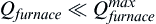

Q_{f u r n a c e} ≪ Q_{f u r n a c e}^{m a x}

$Q_{f u r n a c e} ≪ Q_{f u r n a c e}^{m a x}$

4. The hydraulic limit of the network was never reached.

Parameters that characterize the fouling behavior in each unit were estimated to fit the performance of the base-case configuration C1. Once the fouling behavior was captured, the same values were used to assess alternative network retrofit configurations, with the goal of increasing overall energy recovery. By analyzing the stream temperatures reported in Coletti et al. (2011), it was decided to study the effect of adding an extra heat exchange area to the network to recover more energy from the residue stream (highlighted in red in Figure 5.49). This can be done, for example, by adding an extra unit E-07x, identical to E-07 in geometry. The question then becomes where the extra area should be added to maximize energy recovery while taking into account fouling dynamics. Three alternative network structures were considered by Coletti et al. (2011). The first broadly followed pinch rules to maximize energy recovery based on clean exchanger performance and the remaining two sought to improve the energy recovery while also taking into account the fouling behavior. In summary, the following alternative configurations were studied (Figure 5.49):

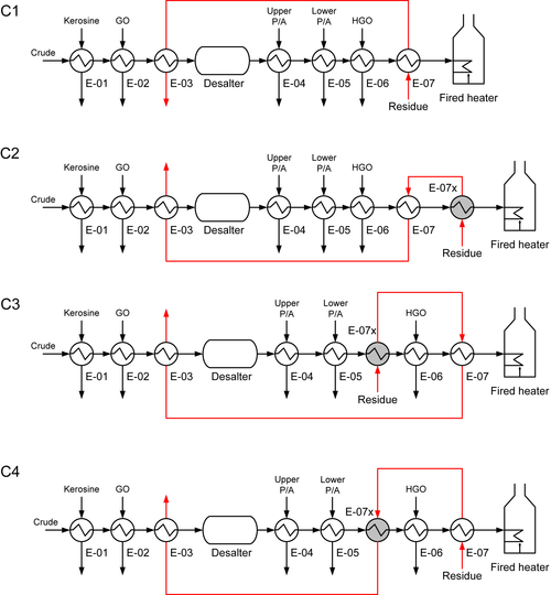
Figure 5.49 HEN2 network configurations considered. Adapted from Coletti et al. (2011).

• Configuration C2, shown in. In this configuration, pinch rules for maximum energy recovery were applied. As a result, E-07x was added between the E-07 and the furnace, at the hottest position in the network. The hot residue stream is matched with the crude at its highest temperature. Although this ensures maximum heat recovery under clean conditions, over time fouling is expected to penalize the overall heat recovery of the network as the wall temperatures, on which fouling depends, are also maximized.

• Configuration C3 in. This configuration goes against traditional pinch rules by matching the hot residue stream with the crude at an intermediate temperature (at the exit of E-05). The residue stream enters the extra unit E-07x, placed between E-05 and E-06 and subsequently enters E-07 and E-03. As a result, heat recovery under clean conditions is expected to be less than that achievable with configuration C3; however, the crude at the highest temperature exchanges heat with a lower temperature residue stream.

• Configuration C4 in. This considers the residue entering first unit E-07 as in the base-case structure and then unit E-07x, which is placed between E-05 and E-06 as in structure C3.

Note that the design of the extra heat exchanger was not optimized for each configuration to provide a more direct comparison of the effect of adding the same area in different positions of the network. The performance given by the different designs is assessed below by the use of the KPI illustrated in the previous section.

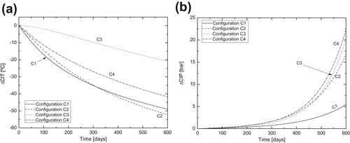
By inspecting the values of the CIT for the base case and the three retrofit options (Figure 5.50) it can be seen that for configurations C2 and C4 the CIT under clean conditions (i.e., t = 0) is over 13 °C higher than that achieved in C1, indicating a good extra energy recovery. Conversely, the initial CIT in configuration C3 is 3.5 °C lower than the base-case C1, despite the extra heat transfer area available. This can be explained with the fall in performance of the existing units E6 and E7 caused by the reduced temperature driving force. Over time, however, things change significantly because of fouling. Fouling rates in E-07 are highest for configurations C3 and C4, and lowest for C1 and C2. Unit E-07x fouls more in C2 than in C3 and C4. As a result, after less than a month of operations, the CIT in C3 is maintained at a higher value compared to that of the base-case C1. After 150 days C3 starts recovering more energy than C2. After ca. 300 days, the CIT in the retrofit structure C4 also falls below that of C3. The structure generated according to pinch rules, C2, results in the worst performance over a long time.

Figure 5.51(a) shows that the drop in CIT over time from clean conditions is drastic for C1 and C2 whereas C4 performs better. Configuration C3 in particular is the one that suffers the least from the decrease in CIT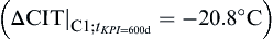

({Δ CIT |}_{C 1; t_{K P I = 600 d}} = - 20.8 ° C)

$({Δ CIT |}_{C 1; t_{K P I = 600 d}} = - 20.8 ° C)$

Figure 5.50 Coil inlet temperature (CIT) for the base-case and the three alternative network configurations. Reproduced with permission from Coletti et al., Effects of fouling on performance of retrofitted heat exchanger networks; a thermo-hydraulic based analysis, 2011. Comput. Chem. Eng. 35 (5), 907–917.

The networks perform very much differently also from a hydraulic point of view. Figure 5.51(b) shows the increase in pressure drops with respect to clean conditions for each configuration considered (ΔCIP, calculated with Equation (5.99)). Since the existing network C1 has one unit less (E-07x), it has a lower total pressure drop and a lower ΔCIP compared to the others

({Δ CIP |}_{C 1; t_{K P I = 600 d}} = 5.4 bar)

$({Δ CIP |}_{C 1; t_{K P I = 600 d}} = 5.4 bar)$

. Among the three proposed retrofits, C4 performs the worst, with

{Δ CIP |}_{C 4; t_{K P I = 600 d}} = 22.3 bar

${Δ CIP |}_{C 4; t_{K P I = 600 d}} = 22.3 bar$

Figure 5.51 ΔCIT (a) and ΔCIP (b) for the different network configurations considered. Reproduced with permission from Coletti et al., Effects of fouling on performance of retrofitted heat exchanger networks; a thermo-hydraulic based analysis, 2011. Comput. Chem. Eng. 35 (5), 907–917.

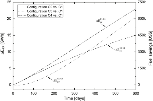
Although the analysis of the CIT and CIP highlights the importance of considering fouling dynamics in the retrofit of PHT networks, it is not sufficient to assess which structure, among those proposed, provides the largest overall amount of energy recovered over time. Figure 5.52 shows the (cumulative) amount of extra energy recovered by the network through one of the three proposed retrofits, as variation in the energy required in the furnace, with respect to the base case. Configuration C3 has a negative impact on the overall energy recovered by the network under clean conditions as confirmed by the fact that

Δ E_{F F}^{C 1 - C 3}

$Δ E_{F F}^{C 1 - C 3}$

is negative for ca. the first 50 days of operations (Figure 5.52). However, after roughly a year of operations configuration C3 starts performing better than C2, the configuration proposed following pinch rules. By analyzing Figure 5.52 another important aspect can be unveiled. While the CIT in configuration C3 becomes larger than that in C4 after ca. 300 days, the cumulative extra energy recovered by the latter is constantly larger than that recovered by the former. One of the key observations enabled by the use of the model is that the position of the extra unit and its fouling behavior are paramount for the overall performance of the network. In configuration C4, the fouling resistance in E-07 increases with respect to the base case (the tube-side temperatures are higher) but it results in the lowest fouling resistance in E-07x. As a result, configuration C4 is capable of saving over 22.5 GWh after 600 days in furnace fuel alone

({Δ E_{F F}^{C 1 - C 4} |}_{t_{K P I = 600 d}} = 22.7 GWh)

$({Δ E_{F F}^{C 1 - C 4} |}_{t_{K P I = 600 d}} = 22.7 GWh)$

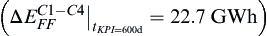. In economic terms, savings in fuel costs alone are shown on the right axis of Figure 5.52.

Figure 5.52 Extra energy recovered by each configuration proposed with respect to the base case. The right axis shows the equivalent savings in terms of fuel burnt in the furnace, $S v_{F F}^{C 1 - C j}$ $S v_{F F}^{C 1 - C j}$ . Reproduced with permission from Coletti et al., Effects of fouling on performance of retrofitted heat exchanger networks; a thermo-hydraulic based analysis, 2011. Comput. Chem. Eng. 35 (5), 907–917.

Table 5.15

KPI summary at t_KPI = 600 days for the three proposed retrofits

#	KPI	Description	Units	C1	C2	C3	C4
01	ΔCIT	CIT drop	°C	−49.0	−52.2	−20.9	−41.7
02r	Sv_FF	Fuel savings	US$	–	451,000	616,000	961,000
03r	$S v_{C O_{2}}$ $S v_{C O_{2}}$	CO₂ savings	US$	–	110,000	150,000	168,000
04	t_PL	Production loss start	Days	∞	∞	∞	∞
05	C_PL	Production loss	US$	0	0	0	0
05r	Sv_PL	Production loss savings	US$	0	0	0	0
06	ΔCIP	CIP increase	Bar	5.4	16.7	20.2	22.3
07r	Sv_PP	Pumping savings	US$	<1000	<1000	<1000	<1000
08r	Sv_tot	Total costs	US$	–	561,000	766,000	859,000

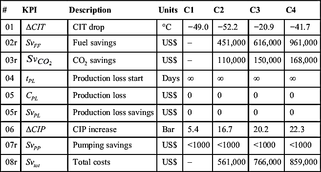
Adapted from Coletti et al. (2011).

Table 5.15 reports a summary of the KPIs used to comprehensively assess the fouling behavior of the different configurations at t_KPI=600d. With respect to CIT drop, network C2 is the worst performer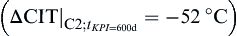

({Δ CIT |}_{C 2; t_{K P I = 600 d}} = - 52 ° C)

$({Δ CIT |}_{C 2; t_{K P I = 600 d}} = - 52 ° C)$

. KPI-02r, Sv_FF, estimated for the different configurations shows that of over US$450,000 in fuel savings can be achieved by using configuration C2 while c. US$600,000 using C3 and ca. US$680,000 using configuration C4. The extra economic benefit of C4 versus C2 is ca. 50%. While after 300 days of operation, the savings at the furnace ranks options are

S v_{F F}^{C 1 - C 4} > S v_{F F}^{C 1 - C2} > S v_{F F}^{C 1 - C3}

$S v_{F F}^{C 1 - C 4} > S v_{F F}^{C 1 - C2} > S v_{F F}^{C 1 - C3}$

, after 600 days the ranking becomes

S v_{F F}^{C 1 - C 4} > S v_{F F}^{C 1 - C3} > S v_{F F}^{C 1 - C2}

$S v_{F F}^{C 1 - C 4} > S v_{F F}^{C 1 - C3} > S v_{F F}^{C 1 - C2}$

. In fuel costs alone, these differences translate in ca. US$230,000 over 600 days between a network structures designed accordingly to pinch rules and one that takes into account fouling. This is considered large for the size of the refinery considered (20,000 bbl day⁻¹). It should be noted that in absolute energy and monetary terms, benefits are expected to be much higher for larger refineries. Moreover, other factors not included in this case study, such as reduction in throughput, could play a crucial role in the choice of the arrangement.

5.4.7. Concluding Remarks

At the beginning of Chapter 5, the vison for a multiscale model of refinery heat exchangers undergoing crude oil fouling was illustrated. This envisaged the integration of thermodynamic and molecular models with fluid-dynamic and industrial-scale models to enable accurate and detailed predictions of fouling deposition from crude oils. The following Section 5.2 and Section 5.3 discussed two of the building blocks of this vision (namely thermodynamic and fundamental transport modeling). Although significant progress has been made in these areas, more development is required to enable the overall vison to be achieved and to make use at industrial scale of the predictive features of such an approach.

This final section of the chapter presented a modeling approach which is in itself a multiscale one. Although it incorporates less descriptive submodels for thermodynamics and fluid dynamics, the model is able to capture some of the complex phenomena described in Chapter 2, such as deposit aging, to a level of detail and accuracy that enables immediate and practical use in industrial settings. The parameters for such submodels may be obtained directly from macro-level experiments (such as those described in Chapter 3) or refinery data.

The distinctive features of the model allow to calculate the thermal resistance and thickness of the fouling layer along the tube as well as its interactions with heat transfer and fluid flow. The distributed nature of the model allows to identify critical zones where deposition is particularly severe and proposing geometries that mitigate fouling. Such features together with the implementation in a commercial process simulator make the model, commercialized by Hexxcell Ltd., a user-friendly and powerful tool.

The excellent agreement (less than 2% error) between model predictions and primary plant measurements (i.e., temperatures) from different refineries over extended Periods of time (i.e., up to 16 months) gives the necessary confidence that the model is capable of representing the performance of individual heat exchangers and entire networks in a reliable way. As a result, the model can be used with confidence to precisely quantify energy losses caused by fouling and propose retrofit options to minimize them at both individual heat exchanger and network levels.

..................Content has been hidden....................

You can't read the all page of ebook, please click here login for view all page.

Table of Contents for 5.4. Industrial Scale High-Fidelity Modeling

Create new playlist

Sign In

Sign Up

5.4. Industrial Scale High-Fidelity Modeling

5.4.1. Governing Equations

5.4.1.1. Thermal Model

5.4.1.2. Fouling Model

5.4.1.3. Hydraulics

5.4.2. Parameter Estimation Procedure

5.4.3. Plant Data

5.4.4. Implementation

5.4.5. Model Validation and Results for Individual Heat Exchangers

5.4.5.1. Model Results and Predictions for RA-E01

5.4.5.2. Model Results and Predictions for Other Heat Exchangers

5.4.5.3. Retrofit of Unit RA-E01

5.4.6. Whole Preheat Train Case Study

5.4.6.1. Assessment of Network Performance: Key Performance Indicators

5.4.6.1.1. Fuel Costs

5.4.6.1.2. Emission Costs

5.4.6.1.3. Production Loss

5.4.6.1.4. Assessment of Hydraulic Efficiency

5.4.6.1.5. Overall Fouling Costs

5.4.6.2. Case Study on Entire Preheat Train

5.4.7. Concluding Remarks

Table of Contents for
5.4. Industrial Scale High-Fidelity Modeling