
Random Number Generation
Introduction
In this chapter, we begin to get into actual cryptography by studying one of the most crucial but often hard to describe components of any modern cryptosystem: the random bit generator.
Many algorithms depend on being able to collect bits or, more collectively, numbers that are difficult for an observer to guess or predict for the sake of security. For example, as we shall see, the RSA algorithm requires two random primes to make the public key hard to break. Similarly, protocols based on (say) symmetric ciphers require random symmetric keys an attacker cannot learn. In essence, no cryptography can take place without random bits. This is because our algorithms are public and only specific variables are private. Think of it as solving linear equations: if I want to stop you from solving a system of four equations, I have to make sure you only know at most three independent variables. While modern cryptography is more complex than a simple linear system, the idea is the same.
Throughout this chapter, we refer to both random bit generators and random number generators. For all intents and purposes, they are the same. That is, any bit generator can have its bits concatenated to form a number, and any number can be split into at least one bit if not more.
When we say random bit generator, we are usually talking about a deterministic algorithm such as a Pseudo Random Number Generator (PRNG) also known as a Deterministic Random Bit Generator (DRBG in NIST terms). These algorithms are deterministic because they run as software or hardware (FSM) algorithms that follow a set of rules accurately. On the face of it, this sounds rather contradictory to the concept of a random bit generator to be deterministic. However, as it turns out, PRNGs are highly practical and provide real security guarantees in both theory and practice. On the upside, PRNGs are typically very fast, but this comes at a price. They require some outside source to seed them with entropy. That is, some part of the PRNG deterministic state must be unpredictable to an outside observer.
This hole is where the random bit generators come into action. Their sole purpose is to kick-start a PRNG so it can stretch the fixed size seed into a longer size string of random bits. Often, we refer to this stretching as bit extraction.
Concept of Random
We have debated the concept and existence of true randomness for many years. Something, such as an event, that is random cannot be predicted with more probability than a given model will allow. There has been a debate running throughout the ages on randomness. Some have claimed that some events cannot be fully modeled without disturbing the state (such as observing the spin of photons) and therefore can be random, while others claim at some level all influential variables controlling an event can be modeled. The debate has pretty much been resolved. Quantum mechanics has shown us that randomness does in fact exist in the real world, and is a critical part of the rules that govern our universe. (For interest, the Bell Inequality gives us good reason to believe there are no “deeper” systems that would explain the perceived randomness in the universe. Wikipedia is your friend.)
It is not an embellishment to say that the very reason the floor is solid is direct proof that uncertainty exists in the universe. Does it ever strike you as odd that electrons are never found sitting on the surface of the nucleus of the atom, despite the fact opposite charges should attract? The reason for this is that there is a fundamental uncertainty in the universe. Quantum theory says that if I know the position on an electron to a certain degree, I must be uncertain of its momentum to some degree.
When you take this principle to its logical conclusion, you are able to justify the existence of a stable atom in the presence of attractive charges. The fact you are here to read this chapter, as we are here to write it, is made possible by the fundamental uncertainty present in the universe.
Wow, this is heavy stuff and we are only on the second page of this chapter. Do not despair; the fact that there is real uncertainty in the world does not preclude us trying to understand it in a scientific and well-contained way.
Claude Shannon gave us the tools to do this in his groundbreaking paper published in 1949. In it, he said that being uncertain of a result implied there was information to be had in knowing it. This offends common sense, but it is easy to see why it is true.
Consider there’s a program that has printed a million “a”s to the screen. How sure are you that the next letter from the program will be “a?” We would say that based on what you’ve seen, the chances of the next letter being “a” are very high indeed. Of course, you can’t be truly certain that the next letter is “a” until you have observed it. So, what would it tell us if there was another “a?” Not a lot really; we already knew there was going to be an “a” with very high probability. The amount of information that “a” contains, therefore, is not very much.
These arguments lead into a concept called entropy or the uncertainty of an event—rather complicated but trivial to explain. Consider a coin toss. The coin has two sides, and given that the coin is symmetric through its center (when lying flat), you would expect it to land on either face with a probability of 50%. The amount of entropy in this event is said to be one bit, which comes from the equation E = –log2(p), or in this case –log2(0.5) = 1. This is a bit simplistic; the amount of entropy in this event can be determined using a formula derived by Bell Labs’ Claude Shannon in 1949. The event (the coin toss) can have a number of outcomes (in this case, either heads or tails). The entropy associated with each outcome is –log2(p)1, where p is the probability of that particular outcome. The overall entropy is just the weighted average of the entropy of all the possible outcomes. Since there are two possible outcomes, and their entropy is the same, their average is simply E = –log2(0.5) = 1 bit. Entropy in this case is another way of expressing uncertainty. That is, if you wrote down an infinite stream of coin toss outcomes, the theory would tell us that you could not represent the list of outcomes with anything less than one bit per toss on average. The reader is encouraged to read up on Arithmetic Encoding to see how we can compress binary strings that are biased.
This, however, assumes that there are influences on the coin toss that we cannot predict or model. In this case, it is actually not true. Given an average rotational speed and height, it is possible to predict the coin toss with a probability higher than 50%. This does not mean that the coin toss has zero entropy; in fact, even with a semi-accurate model it is likely still very close to one bit per toss. The key concept here is how to model entropy.
So, what is “random?” People have probably written many philosophy papers on that question. Being scientists, we find the best way to approach this is from the computer science angle: a string of digits is random if there is no program shorter than it that can describe its form.
This is called Kolmogorov complexity, and to cover this in depth here is beyond the scope of this text. The interested reader should consult The Quest for Omega by G.J. Chaitin. The e-book is available at www.arxiv.org/abs/math.HO/0404335.
What is in scope is how to create nondeterministic (from the software point of view) random bit generators, which we shall see in the upcoming section. First, we have to determine how we can observe the entropy in a stream of events.
Measuring Entropy
The first thing we need to be able to do before we can construct a random bit generator is have a method or methods that can estimate how much entropy we are actually generating with every bit generated. This allows us to use carefully the RNG to seed a PRNG with the assumption that it has some minimum amount of entropy in the state.
Note clearly that we said estimate, not determine. There are many known useful RNG tests; however, there is no short list of ways of modeling a given subset of random bits. Strictly speaking, for any bit sequence of length L bits, you would have to test all generators of length L–1 bits or less to see if they can generate the sequence. If they can, then the L bits actually have L–1 (or less) bits of entropy.
In fact, many RNG tests do not even count entropy, at least not directly. Instead, many tests are simply simulations known as Monte Carlo simulations. They run a well-studied simulation using the RNG output at critical decision points to change the outcome. In addition to simulations, there are predictors that observe RNG output bits and use that to try to simulate the events that are generating the bits.
It is often much easier to predict the output of a PRNGs than a block cipher or hash doing the same job. The fact that PRNGS typically use fewer operations per byte than a block cipher means there are less operations per byte to actually secure the information. It is simplistic to say that this, in itself, is the cause of weakness, but this is how it can be understood intuitively. Since PRNGS are often used to seed other cryptographic primitives, such as block ciphers or message authentication codes, it is worth pointing out that someone who breaks the PRNG may well be able to take down the rest of the system.
Various programs such as DIEHARD and ENT have surfaced on the Internet over the years (DIEHARD being particularly popular—www.arxiv.org/abs/math.HO/0404335) that run a variety of simulations and predictors. While they are usually good at pointing out flawed designs, they are not good at pointing out good ones. That is, an algorithm that passes one, or even all, of these tests can still be flawed and insecure for cryptographic purposes. That said, we shall not dismiss them outright and explore some basic tests that we can apply.
A few key tests are useful when designing a RNG. These are by no means an exhaustive list of tests, but are sufficient to quickly filter out RNGs.
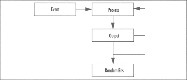
Bit Count
The “bit count” test simply counts the number of zeroes and ones. Ideally, you would expect an even distribution over a large stream of bits. This test immediately rules out any RNG that is biased toward one bit or another.
Word Count
Like the bit count, this test counts the number of k-bit words. Usually, this should be applied for values of k from two through 16. Over a sufficiently large stream you should expect to see any k-bit word occurring with a probability of 1/2k. This test rules out oscillations in the RNG; for example, the stream 01010101 … will pass the bit count but fail the word count for k=2. The stream 001110001110 … will pass both the bit count and for k=2, but fail at k=3 and so on.
Gap Space Count
This test looks for the size of the gaps between the zero bits (or between the one bits depending how you want to look at it). For example, the string 00 has a gap of zero, 010 has a gap of one, and so on. Over a sufficiently large stream you would expect a gap of k bits to occur with a probability of 1/2k+l. This test is designed to catch RNGs that latch (even for a short period) to a given value after a clock period has finished.
Autocorrelation Test
This test tries to determine if a subset of bits is related to another subset from the same string. Formally defined for continuous streams, it can be adopted for finite discrete signals as well. The following equation defines the autocorrelation.
![]()
Where x is the signal being observed and R(j) is the autocorrelation coefficient for the lag j. Before we get too far ahead of ourselves, let us examine some terminology we will use in this section. Two items are correlated if they are more similar (related) than unlike. For example, the strings 1111 and 1110 are similar, but by that token, so are 1111 and 0000, as the second is just the exact opposite of the first. Two items are uncorrelated if they have equal amounts of distinction and similarity. For example, the strings 1100 and 1010 are perfectly uncorrelated.
In the discrete world where samples are bits and take on the values {0, 1}, we must map them first to the values {–1, 1} before applying the transform. If we do not, the autocorrelation function will tend toward zero for correlated samples (which are the exact opposites).
There is another more hardware friendly solution, which is to sum the XOR difference of the two. The new autocorrelation function becomes
![]()
This will tend toward n/2 for uncorrelated streams and toward 0 or n for correlated streams. Applying this to a finite stream now becomes tricky. What are the samples values below the zero index? The typical solution is to start summation from j onward and look to have a summation close to (n–j)/2 instead.
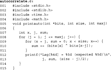
This function prints the autocorrelation coefficients for an array of samples up to a maximum lag. Let’s consider a simple biased PRNG.
This generator will output the last bit with a probability of 50%, and otherwise will output a random bit. Let’s examine the data through the autocorrelation test.
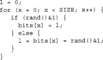
![]()
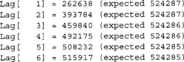
This was over 1048576 samples (220). We can see that we are far from ideal in the first eight lags listed. Now consider the test on just rand ( ) & 1.
As we can see, the autocorrelation values are closer to the expected mean than before. The conclusion from this is experiment would be that the former is a bad bit generator and the latter is more appropriate. Keep in mind this test does not mean the latter is ideal for use as a RNG. The rand() function from glibc is certainly not a secure PRNG and has a very small internal state. This is a common mistake; do not make it.
One downside to this trivial implementation is that it requires a huge buffer and cannot be run on the fly. In particular, it would be nice to run the test while the RNG is active to ensure it does not start producing correlated outputs. It turns out a windowed correlation test is fairly simple to implement as well.

In this case, we defined 16 taps (MAXLAG), and this function will process one bit at a time through the autocorrelation function. It does not output a result, but instead updates the global correlation array. This is essentially a shift register with a parallel summation operation. It is actually well suited to both hardware implementation and SIMD software (especially with longer LAG values). This test functions best only on longer streams of bits. The default window will populate with zero bits, which may or may not correlate to the bits being added. In general, avoid applying the autocorrelation test to strings fewer than at least a couple thousand bits.
How Bad Can It Be?
In all the tests mentioned previously, you know the “correct” answer, but you won’t often get it. For example, if you toss a perfect coin 20 times, you expect 10 heads. But what if you get 11, or only 9? Does that mean the coin was biased? In fact, of all the 220 (1048576) possible (and equally likely) outcomes of your 20 coin tosses, only 184756, about 18%, actually have exactly 10 heads.
Statistics texts can tell us just how (un)likely a particular set of output bits is, based on the assumption that the generator is good. In practice, though, a little common sense will often be enough; while even 8 heads isn’t that unlikely, 2 is definitely unexpected, and 20 pretty much convinces you it was a two-headed coin. The more data you use for the test, the more reliable your intuition should be.
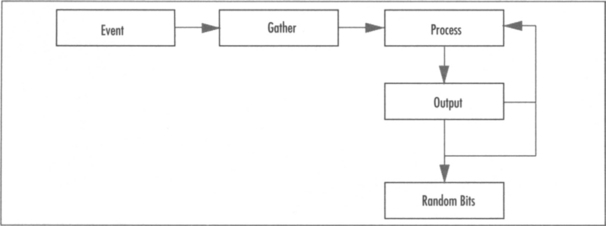
RNG Design
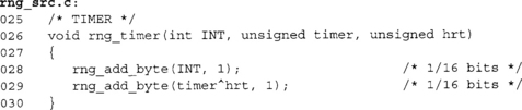
Most RNGs in practice are designed around some event gathering process that follows the pipeline described in Figure 3.1.There are no real standards for RNG design, since the standards bodies tend to focus more on the deterministic side (e.g., PRNGs). Several classic RNGs such as the Yarrow and Fortuna designs (which we will cover later) are flexible and designed by some of the best cryptographers in the field. However, what we truly want is a simple yet effective RNG.
For this task, we will borrow from the Linux kernel RNG. It is a particularly good model, as it is integrated inside the kernel as opposed to an external entity sitting in user space. As such, it has to behave itself with respect to stack, heap, and CPU time resource usage.
The typical RNG workflow can be broken into the following discrete steps: events, gathering, processing, and output feedback. Not all RNGs follow this overall design concept, but it is fairly common.
The first misconception people tend to have is to assume that RNGs feed off some random source like interrupt timers and return output directly. In reality, most entropy sources are, at least from an information theoretic viewpoint, less than ideal. The goal of the RNG is to extract the entropy from the input events (the seed data) and return only as many random bits to the caller as entropy bits with which it had been seeded. This is actually the only key difference in practice between an RNG and a PRNG.
An RNG also differs from a PRNG in that it is supposed to be fed constantly seeding entropy. A PRNG is meant to be seeded once (or seldom) and then outputs many more bits than the entropy of its internal state. This key difference limits the use of an RNG in situations where seeding events are hard to come by or are of low entropy.
RNG Events
An RNG event is what the RNG will be observing to try to extract entropy from. They are events in systems that do not occur with highly predictable intervals or states. The goal of the RNG is then to capture the event, gather the entropy available, and pass it on to be processed into the RNG internal state.
Events come in all shapes and sizes. What events you use for an RNG depends highly on for what the platform is being developed. The first low-hanging fruit in terms of a desktop or server platform are hardware interrupts, such as those caused by keyboard, mouse, timer (drift), network, and storage devices. Some, if not all, of these are available on most desktop and server platforms in one form of another. Even on embedded platforms with network connections, they are readily available.
Other typical sources are timer skews, analogue-to-digital conversion noise, and diode leakage. Let us first consider the desktop and server platforms.
Hardware Interrupts
In virtually all platforms with hardware interrupts, the process of triggering an interrupt is fairly consistent. In devices capable of asserting an interrupt, they raise a signal (usually a dedicated pin) that a controller (such as the Programmable Interrupt Controller (PIC)) detects, prioritizes, and then signals the processor. The processor detects the interrupt, stops processing the current task, and swaps to a kernel handler, which then acknowledges the interrupt and processes the event. After handling the event the interrupt handler returns control to the interrupted task and processing resumes as normal.
It is inside the handler where we will observe and gather the entropy from the event. This additional step raises a concern, or it should raise a concern for most developers, since the latency of the interrupt handler must be minimal to maintain system performance. If a 1 kHz timer interrupt takes 10,000 cycles to process, it is effectively stealing 10,000,000 cycles every second from the users’ tasks (that is, dropping 10 MHz off your processor’s speed). Interrupts have to be fast, which implies that what we do to “gather” the entropy must be trivial, perhaps at most a memory copy. This is why there are distinct gather and process steps in the RNG construction. The processing will occur later, usually as a result of a read from the RNG from a user task.
The first piece of entropy we can gather from the interrupt handler is which interrupt this is; that (say) a timer interrupt occurred is not highly uncertain, that it occurred between (say) two different interrupts is, especially in systems under load. Note that timers are tricky to use in RNG construction, which we shall cover shortly.
The next piece of entropy is the data associated with event. For example, for a keyboard interrupt the actual key pressed, for a network interrupt the frame, for a mouse interrupt the co-ordinates or input stream, and so on. (Clearly, copying entire frames on systems under load would be a significant performance bottleneck. Some level of filtering has to take place here.)
The last useful piece of entropy is the capturing of a high-resolution free running counter. This is extremely useful for systems where the load is not high enough for combinations of interrupts to have enough entropy. For example, that a network interrupt occurred may not have a lot of entropy. The exact clock tick at which it occurred can be in doubt and therefore have entropy. This is particularly practical where the clock being read is free running and not tied to the task scheduling or interrupt scheduling process. On x86 processors, the RDTSC instruction can be used for this process as it is essentially a very high-precision free running counter not affected by bus timing, device timing, or even the processor’s instruction flow. This last source of entropy is a form of timer skew, which we shall cover in the next section.
All three pieces of information alone may yield very little entropy, but together will usually have a nonzero amount of entropy sufficient for gathering and further processing.
Timer Skew
Timer skew occurs when two or more circuits are not phase locked; they may oscillate at the same frequency, but the start and stop of a period may shift depending on many factors such as voltage and temperature, to name two. In digital equipment, this usually is combated with the use of reducing the number of distinct clocks, PLL devices, and self-clocking (such as the HyperTransport bus).
In software, it is usually hard to come by timers that are distinct and not locked to one another. For example, the PCI clock should be in sync with every device on the PCI bus. It should also be locked to that of the Southbridge that connects to the PCI controllers, and so on.
In the x86 world, it turns out there is at least one sufficiently useful (albeit slow) source. Yet again, the RDTSC instruction is used. The processor’s timer, at least for Intel and AMD, is not directly tied to the PIT or ACPI timers. Entropy therefore can be extracted with a fairly simple loop.
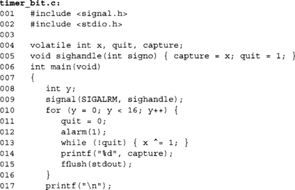
![]()
This example displays 16 bits and then returns to the shell. In this example, the XOR ‘ing of the x variable with one produces a high frequency clock oscillating between 0 and 1 as fast as the processor can decode, schedule, execute, and retire the operation. The exact frequency of this clock for a given one-second period depends on many factors, including cache contents, other interrupts, other tasks pre-empting this task, and where the processor is in executing the loop when the alarm signals.
On the x86 platform, the while loop would essentially resemble
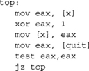
At first, it may seem odd that the compiler would produce three opcodes for the XOR operation when a single XOR with a memory operand would suffice. However, the “x ^ = 1” operation actually defines three atomic operations since x is volatile, a load, an XOR, and a store. From the program’s point of view, even with a signal by time we exit the while loop the entire XOR statement has executed. This is why the signal handler will capture the value of x before setting the quit flag.
The interrupt (or in this case a signal) can stop the program flow before any one of the instructions. Only one of them actually updates the value of x in memory where the signal handler can see it. Figure 3.2 shows some sample outputs produced on an Opteron workstation.
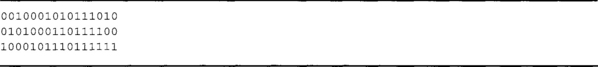
If we continued, we would likely see that there is some form of bias, but at the very least, the entropy is not zero. One problem, however, is that this generator is extremely slow. It takes one second per bit, and the entropy per output is likely nowhere close to one bit per bit. A more conservative estimate would be that there is at most 0.1 bits of entropy per bit output. This means that for a 128-bit sequence, it would take 1280 seconds, or nearly 22 minutes.
One solution would be to decrease the length of the delay on the alarm. However, if we sample for too short a period the likelihood of a frequency shift will be decreased, lowering the entropy of the output. That is, it is more likely that two free running counters remain in synchronization for a shorter period of time than a longer period of time.
Fine tuning the delay is beyond the goal of this text. Every platform, even in the x86 world, and every implementation is different. The power supply, location, and quality of the onboard components will affect how much and how often phase lock between clocks is lost.
In hardware, such situations can be recreated for profit but are typically hard to incorporate. Two clocks, fed from the same power source (or rail), will be exposed to nearly the same voltage provided they are of the same design and have equal length power traces. In effect, you would not expect them to be in phase lock, but would also not expect them to experience a large amount of drift, certainly over a short period of time. It is true that no two clocks will be exactly the same; however, for the purposes of an RNG they will most likely be similar enough that any uncertainty in their states is far too little to be useful. Hardware clocks must be fed from different power rails, such as two distinct batteries. This alone makes them hard to incorporate on a cost basis.
The most practical form of this entropy collection would be with interrupts alongside with a high-resolution free running timer. Even the regularly scheduled system timer interrupt should be gathered with this high precision timer.
Analogue to Digital Errors
Analogue to Digital converts (ADC) capture an input waveform and then quantize and digitize the signal. The result is usually a Pulse Code Modulation stream where groups of bits represent the signal strength at a discrete moment in time. These are typically found in soundcards as microphone or line-in components, on TV tuner decoders, and in wireless radio devices.
As in the case of the timer skews, we are trying to exploit any otherwise perceivable failings in the circuit to extract entropy. The most obvious source is the least significant bit of the samples, which can settle on one value or another depending on when the sample as latched, the comparative voltage going to the ADC, and other environmental noises. In fact, timer skew (signaling when to latch the sample) can add entropy to the retrieved samples.
As an experiment, consider playing a CD and recording the output from a microphone while sitting in a properly isolated sound studio. The chances are very high that the two bit streams will not agree exactly. The cross-correlation between the two will be very strong, especially if the equipment is of high quality. However, even in the best of situations there is still limited entropy to be had.
Another experiment that is easier to attempt is to record on your desktop with (or without) a microphone attached the ambient noise where your machine is located. Even without a microphone, the sound codec on a Tyan 2877 will detect low levels of noise through the ADC. The samples are extremely small, but even in this extreme case there is entropy to be gathered. Ideally, it is best if a recording device such as a microphone is attached so it can capture environmental ambient noise as well.
In practice, ADCs are harder to use in desktop and server setups. They are more likely to be available in custom embedded designs where such components can be used without conflicting with the user. For example, if your OS started capturing audio while you were trying to use the sound card, it may be bothersome. In terms of the data we wish to gather, it is only the least significant bit. This reduces the storage requirement of the gathering process significantly.
RNG Data Gathering
Now that we know a few sources where entropy is to be had, we must design a quick way of collecting it. The goal of the gathering step is to reduce the latency of the event stage such that interrupts are serviced in a reasonably well controlled amount of time.
Effectively, the gathering stage collects entropy and feeds it to the processing stages when not servicing an interrupt. We are pushing when we have to do something meaningful with the entropy not removing the step altogether.
The logical first step is to have a block of memory pre-allocated in which we can dump the data. However, this yields a new problem. The block of memory will be a fixed size, which means that when the block is full, new inputs must either be ignored or the block must be sent to processing. Simply dropping new (or older) events to ensure the buffer is not overflowed is not an option.
An attacker who knows that entropy can be discarded will simply try to trigger a series of low entropy events to ensure the collected data is of low quality. The Linux kernel approaches this problem by using a two-stage processing algorithm. In the first stage, they mix the entropy with an entropy preserving Linear Feedback Shift Register (LFSR). An LFSR is effectively a PRNG device that produces outputs as a linear combination of its internal state. (Why use an LFSR? Suppose we just XORed the bits that came off the devices and there was a bias. The bias would tend to collect on distinct bits in the dumping area. The LFSR, while not perfect, is quick way to make sure the bias is spread across the memory range.) In the Linux kernel, they step the LFSR but instead of just updating the state of the LFSR with a linear combination of itself, they XOR in bits from the events gathered.
The XOR operation is particularly useful for this, as it is what is known as entropy preserving, or simply put, a balanced operation. Obviously, your entropy cannot exceed the size of the state. However, if the entropy of the state is full, it cannot be decreased regardless of the input. For example, consider the One Time Pad (OTP). In an OTP, even if the plaintext is of very low entropy such as English text, the output ciphertext will have exactly one bit of entropy per bit.
LFSR Basics
LFSRs are also particularly useful for this step as they are fast to implement. The basic LFSR is composed of an L-bit register that is shifted once and the lost bit is XOR’ed against select bits of the shifted register. The bits chosen are known as “tap bits”. For example,
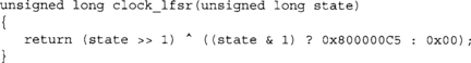
This function produces a 32-bit LFSR with a tap pattern 0x800000C5 (bits 31, 7, 6, 2, and 0). Now, to shift in RNG data we could simply do the following,
This function would be called for every bit in the gathering block until it is empty. As the LFSR is entropy preserving, at most this construction will yield 32 bits of entropy in the state regardless of how many seed bits you feed—far too little to be of any cryptographic significance and must be added as part of a larger pool.
Table-based LFSRs
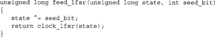
Clocking an LFSR one bit at a time is a very slow operation when adding several bytes. It is far too slow for servicing an interrupt. It turns out we do not have to clock LFSRs one bit a time. In fact, we can step them any number of bits, and in particular, with lookup tables the entire operation can be done without branches (the test on the LSB). Strictly speaking, we could use an LFSR over a different field such as extension fields of the form GF(pk)m[x]. However, these are out of the scope of this book so we shall cautiously avoid them.
The most useful quantity to clock by is by eight bits, which allows us to merge a byte of seed data a time. It also keeps the table size small at one kilobyte.
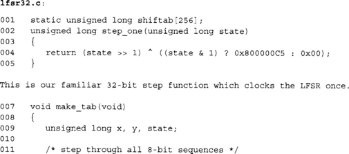

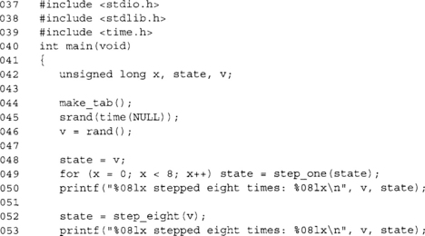
This function creates the 256 entry table shiftab. We run through all 256 lower eight bits and clock the register eight times. The final product of this (line 19) is what we would have XORed against the register.
The first function (line 24) steps the LFSR eight times with no more than a shift, lookup, and an XOR. In practice, this is actually more than eight times faster, as we are moving the conditional XOR from the code path.
The second function (line 30) seeds the LFSR with eight bits in a single function call. It would be exactly equivalent to feeding one bit (from least significant to most significant) with a single stepping function.
![]()
If you don’t believe this trick works, consider this demo program over many runs. Now that we have a more efficient way of updating an LFSR, we can proceed to making it larger.
Large LFSR Implementation
Ideally, from an implementation point of view, you want the LFSR to have two qualities: be short and have very few taps. The shorter the LFSR, the quicker the shift is and the smaller the tables have to be. Additionally, if there are few taps, most of the table will contain zero bits and we can compress it.
However, from a security point of view we want the exact opposite. A larger LFSR can contain more entropy, and the higher number of taps the more widespread the entropy will be in the register. The job of a cryptographer is to know how and where to draw the line between implementation efficiency and security properties.
In the Linux kernel, they use a large LFSR to mix entropy before sending it on for cryptographic processing. This yields several pools that occupy space and pollute the processor’s data cache. Our approach to this is much simpler and just as effective. Instead of having a large LFSR, we will stick with the small 32-bit LFSR and forward it to the processing stage periodically. The actual step of adding the LFSR seed to the processing pool will be as trivial as possible to keep the latency low.
RNG Processing and Output
The purpose of the RNG processing step is to take the seed data and turn it into something you can emit to a caller without compromising the internal state of the RNG. At this point, we’ve only linearly mixed all of our input entropy into the processing block. If we simply handed this over to a caller, they could solve the linear equations for the LFSR and know what events are going on inside the kernel. (Strictly speaking, if the entropy of the pool is the size of the pool this is not a problem. However, in practice this will not always be the case.)
The usual trick for the processing stage is to use a cryptographic one-way hash function to take the seed data and “churn” it into an RNG state from which entropy can be derived. In our construction, we will use the SHA-256 hash function, as it is fairly large and fairly efficient.
The first part of the processing stage is mixing the seed entropy from the gathering stage. We note that the output of SHA-256 is effectively eight 32-bit words. Our processing pool is therefore 256 bits as well. We will use a round-robin process of XOR ‘ing the 32-bit LFSR seed data into one of the eight words of the state. We must collect at least eight words (but possibly more will arrive) from the gathering stage before we can churn the state to produce output.
Actually churning the data is fairly simple. We first XOR in a count of how many times the churn function has been called into the first word of the state. This prevents the RNG from falling into fixed points when used in nonblocking mode (as we will cover briefly). Next, we append the first 23 bytes of the current RNG pool data and hash the 55-byte string to form the new 256-bit entropy pool from which a caller can read to get random bytes. The hash output is then XOR’ed against the 256-bit gather state to help prevent backtracking attacks.
The first odd thing about this is the use of a churn counter. One mode for the RNG to work in is known as “non-blocking mode.” In this mode, we act like a PRNG rather than as an RNG. When the pool is empty, we do not wait for another eight words from the gathering stage; we simply re-churn the existing state, pool, and churn counter. The counter ensures the input to the hash is unique in every churning, preventing fixed points and short cycles. (A fixed point occurs when the output of the hash is equal to the input of the hash, and a short cycle occurs when a collision is found. Both are extremely unlikely to occur, but the cost of avoiding them is so trivial that it is a good safety measure.)
Another oddity is that we only use 23 bytes of the pool instead of all 32. In theory, there is no reason why we cannot use all 32. This choice is a performance concern more than any other. SHA-256 operates (see Chapter 5, “Hash Functions,” for more details) on blocks of 64 bytes at once. A message being hashed is always padded by the hash function with a 0x80 byte followed by the 64-bit encoding of the length of the message. This is a technique known as MD-Strengthening. All we care about are the lengths. Had we used the full 64 bytes, the message would be padded with the nine bytes and require two blocks (of 64 bytes) to be hashed to create the output. Instead, by using 32 bytes of state and 23 bytes of the pool, the 9 bytes of padding fits in one block, which doubles the performance.
You may wonder why we include bytes from the previous output cycle at all. After all, they potentially are given to an attacker to observe. The reason is a matter of more practical security than theoretic. Most RNG reads will be to private buffers for things like RSA key generation or symmetric key selection. The output can still contain entropy. The operation of including it is also free since the SHA-256 hash would have just filled the 23 bytes with zeros. In essence, it does not hurt and can in some circumstances help. Clearly, you still need a fresh source of entropy to use this RNG securely. Recycling the output of the hash does not add to the entropy, it only helps prevent degradation.
Let us put this all together now:
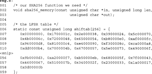
This is the table for the 32-bit LFSR with the taps 0x800000C5. We have trimmed the listing to save space. The full listing is available online.
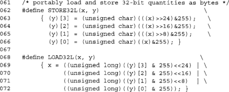
These two macros are new to us, but will come up more and more in subsequent chapters. These macros store and load little endian 32-bit data (resp.) in a portable fashion. This allows us to avoid compatibility issues between platforms.
![]()
This is the RNG internal state. LFSR is the current 32-bit word being accumulated. state is the array of 32-bit words that forms the gathering pool of entropy. word_count counts the number of words that have been added to the state from the LFSR. bit_count counts the number of bits that have been added to the LFSR, and churn_count counts the number of times the churn function has been called.
The bit_count variable is interpreted as a .4 fixed point encoded value. This means that we split the integer into two parts: a 28-bit (on 32-bit platforms, 60 bit on 64-bit platforms) integer and a 4-bit fraction. The value of bit_count literally equates to (bit_count ![]() 4) + (bit_count/16.0) using C syntax. This allows us to add fractions of bits of entropy to the pool.
4) + (bit_count/16.0) using C syntax. This allows us to add fractions of bits of entropy to the pool.
For example, a mouse interrupt may occur, and we add the X,Y buttons and scroll positions to the RNG. We may say all of them have 1 bit of entropy or 0.25 bits per sample fed to the RNG. So, we pass 0.25 * 16 = 4 as the entropy count.
![]()
This is the pool state from the RNG. It contains the data that is to be returned to the caller. The pool array holds up to 32 bytes of RNG output, pool_len indicates how many bytes are left, and pool_idx indicates the next byte to be read from the array.
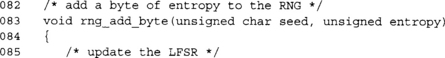
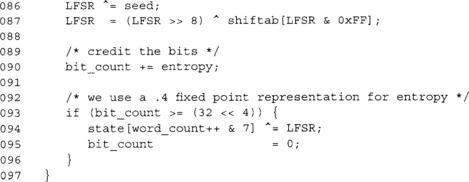
This function adds a byte of entropy from some event to the RNG state. First, we mix in the entropy (line 86) and update the LFSR (line 87). Next, we credit the entropy (line 90) and then check if we can add this LFSR word to the state (line 93). If the entropy count is equal to or greater than 32 bits, we perform the mixing.

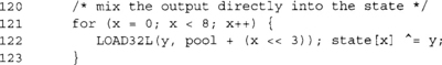
At this point, the local array buf contains 55 bytes of data to be hashed. We recall from earlier that we chose 55 bytes to make this routine as efficient as possible.
![]()
Here we invoke the SHA-256 hash, which hashes the 55 bytes of data in the buf array and stores the 32-byte digest in the pool array. Do not worry too much about how SHA-256 works at this stage.
Note that we are XOR ‘ing the hash output against the state and not replacing it. This helps prevent backtracking attacks. That is, if we simply left the state as is, an attacker who can determine the state from the output can run the PRNG backward or forward. This is less of a problem if the RNG is used in blocking mode.

The read function rng_read() is what a caller would use to return random bytes from the RNG system. It can operate in one of two modes depending on the block argument. If it is nonzero, the function acts like a RNG and only reads as many bytes as the pool has to offer. Unlike a true blocking function, it will return partial reads instead of waiting to fulfill the read. The caller would have to loop if they required traditional blocking functionality. This flexibility is usually a source of errors, as callers do not check the return value of the function. Unfortunately, even an error code returned to the caller would not be noticed unless you significantly altered the code flow of the program (e.g., terminate the application).
If the block variable is zero, the function behaves like a PRNG and will rechurn the existing state and pool regardless of the amount of additional entropy. Provided the state has enough entropy in it, running it as a PRNG for a modest amount of time should be for all purposes just like running a proper RNG.
RNG Estimation
At this point, we know what to gather, how to process it, and how to produce output. What we need now are sources of entropy trapped and a conservative estimate of their entropy. It is important to understand the model for each source to be able to extract entropy from it efficiently. For all of our sources we will feed the interrupt (or device ID) and the least significant byte of a high precision timer to the RNG. After those, we will feed a list of other pieces of data depending on the type of interrupt.
Let us begin with user input devices.
Keyboard and Mouse
The keyboard is fairly easy to trap. We simply want the keyboard scan codes and will feed them to the RNG as a whole. For most platforms, we can assume that scan codes are at most 16 bits long. Adjust accordingly to suit your platform. In the PC world, the keyboard controller sends one byte if the key pressed was one of the typical alphanumeric characters.
When a less frequent key is pressed such as the function keys, arrow keys, or keys on the number pad, the keyboard controller will send two bytes. At the very least, we can assume the least significant byte of the scan code will contain something and upper may not.
In English text, the average character has about 1.3 bits of entropy, taking into account key repeats and other “common” sequences; the lower eight bits of the scan code will likely contain at least 0.5 bits of entropy. The upper eight bits is likely to be zero, so its entropy is estimated at a mere 1/16 bits. Similarly, the interrupt code and high-resolution timer source are given 1/16 bits each as well.
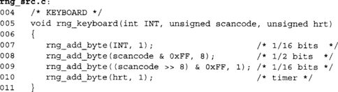
This code is callable from a keyboard, which should pass the interrupt number (or device ID), scancode, and the least significant byte of a high resolution timer. Obviously, where PC AT scan codes are not being used the logic should be changed appropriately. A rough guide is to take the average entropy per character in the host language and divide it by at least two.
For the mouse, we basically use the same principle except instead of a scan code we use the mouse position and status.
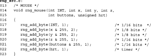
Here we add the lower eight bits of the mouse x-, y-, and z-coordinates (z being the scroll wheel). We estimate that the x and y will give us 1/8th of a bit of entropy since it is only really the least significant bit in which we are interested. For example, move your mouse in a vertical line (pretend you are going to the File menu); it is unlikely that your x-coordinate will vary by any huge amount. It may move slightly left or right of the upward direction, but for the most part it is straight. The entropy would be on when and where the mouse is, and the “error” in the x-coordinate as you try to move the mouse upward.
We assume in this function that the mouse buttons (up to eight) are packed as booleans in the lower eight bits of the button argument. In reality, the button’s state contains very little entropy, as most mouse events are the user trying to locate something on which to click.
Timer
The timer interrupt or system clock can be tapped for entropy as well. Here we are looking for the skew between the two. If your system clock and processor clock are locked (say they are based on one another), you ought to ignore this function.
We estimate that the entropy is 1/16 bits for the XOR of the two timers.
Generic Devices
This last routine is for generic devices such as storage devices or network devices where trapping all of the user data would be far too costly. Instead, we trap the ID of the device that caused the event and the current high-resolution time.
We assume the devices have some form of major:minor identification scheme such as that used by Linux. It could also the USB or PCI device ID if a major/minor is not available, but in that case you would have to update the function to add 16 bits from both major and minor instead of just the lower eight bits.
RNG Setup
A significant problem most platforms face is a lack of entropy when they first boot up. There is not likely to be many (if at all any) events collected by time the first user space program launches.
The Linux solution to this problem is to gather a sizable block of RNG output and write it to a file. On the next bootup, the bits in the file are added to the RNG a rate of one bit per bit. It is important not to use these bits directly as RNG output and to destroy the file as soon as possible.
That approach has security risks since the entire entropy of the RNG can possibly be exposed to attackers if they can read the seed file before it is removed. Obviously, the file would have to be marked as owned by root with permissions 0400.
On platforms on which storage of a seed would be a problem, it may be more appropriate to spend a few seconds reading a device like an ADC. At 8 KHz, a five-second recording of audio should have at least 256 bits of entropy if not more. A simple approach to this would be to collect the five seconds, hash the data with SHA-256, and feed the output to the RNG at a rate of one bit of entropy per bit.
PRNG Algorithms
We now have a good starting point for constructing an RNG if need be. Keep in mind that many platforms such as Windows, the BSDs, and Linux distributions provide kernel level RNG functionality for the user. If possible, use those instead of writing your own.
What we need now, though, are fast sources of entropy. Here, we change entropy from a universal concept to an adversarial concept. From our point of view, it is ok if we can predict the output of the generator, as long as our attackers cannot. If our attackers cannot predict bits, then to them, we are effectively producing random bits.
PRNG Design
From a high-level point of view, a PRNG is much like an RNG. In fact, most popular PRNG algorithms such as Fortuna and the NIST suite are capable of being used as RNGs (when event latency is not a concern).
The process diagram (Figure 3.3) for the typical PRNG is much like that of the RNG, except there is no need for a gather stage. Any input entropy is sent directly to the (higher latency) processing stage and made part of the PRNG state immediately.
The goal of most PRNGs differs from that of RNGs. The desire for high entropy output, at least from an outsider’s point of view, is still present. When we say “outsider,” we mean those who do not know the internal state of the PRNG algorithm. For PRNGs, they are used in systems where there is a ready demand for entropy; in particular, in systems where there is not much processing power available for the output stage. PRNGs must generate high entropy output and must do so efficiently.
Bit Extractors
Formal cryptography calls PRNG algorithms “bit extractors” or “seed lengtheners.” This is because the formal model (Oded Goldreich, Foundations of Cryptography, Basic Tools, Cambridge University Press, 1st Edition) views them as something that literally takes the seed and stretches it to the length desired. Effectively, you are spreading the entropy over the length of the output. The longer the output, the more likely a distinguisher will be able to detect the bits as coming from an algorithm with a specific seed.
Seeding and Lifetime
Just like RNGs, a PRNG must be fed seed data to function as desired. While most PRNGs support re-seeding after they have been initialized, not all do, and it is not a requirement for their security threat model. Some PRNGs such as those based on stream ciphers (RC4, SOBER-128, and SEAL for instance) do not directly support re-seeding and would have to be re-initialized to accept the seed data.
In most applications, the PRNG usefulness can be broken into one of two classifications depending on the application. For many short runtime applications, such as file encryption tools, the PRNG must live for a short period of time and is not sensitive to the length of the output. For longer runtime applications, such as servers and user daemons, the PRNG has a long life and must be properly maintained.
On the short end, we will look at a derivative of the Yarrow PRNG, which is very easy to construct with a block cipher and hash function. It is also relatively quick producing output as fast as the cipher can encrypt blocks. We will also examine the NIST hash based DRBG function, which is more complex but fills the applications where NIST crypto is a must.
On the longer end, we will look at the Fortuna PRNG. It is more complex and difficult to set up, but better suited to running for a length of time. In particular, we will see how the Fortuna design defends against state discovery attacks.
PRNG Attacks
Now that we have what we consider a reasonable looking PRNG, can we pull it apart and break it?
First, we have to understand what breaking it means. The goal of a PRNG is to emit bits (or bytes), which are in all meaningful statistical ways unpredictable. A PRNG would therefore be broken if attackers were able to predict the output more often then they ought to. More precisely, a break has occurred if an algorithm exists that can distinguish the PRNG from random in some feasible amount of time.
A break in a PRNG can occur at one of several spots. We can predict or control the inputs going in as events in an attempt to make sure the entropy in the state is as low as possible. The other way is to backtrack from the output to the internal state and then use low entropy events to trick a user into reading (unblocked) from the PRNG what would be low entropy bytes.
Input Control
First, let us consider controlling the inputs. Any PRNG will fail if its only inputs are from an attacker. Entropy estimation (as attempted by the Linux kernel) is not a sound solution since an attacker may always use a higher order model to generate what the estimator thinks is random data. For example, consider an estimator that only looks at the 0th order statistics; that is, the number of one bits and number of zero bits. An attacker could feed a stream of 01010101 … to the PRNG and it would be none the wiser.
Increasing the model order only means the attacker has to be one step ahead. If we use a 1st order model (counting pair of bits), the attacker could feed 0001101100011011 … and so on. Effectively, if your attacker controls all of your entropy inputs you are going to successfully be attacked regardless of what PRNG design you choose.
This leaves us only to consider the case where the attacker can control some of the inputs. This is easily proven to be thwarted by the following observation. Suppose you send in one bit of entropy (in one bit) to the PRNG and the attacker can successfully send in the appropriate data to the LFSR such that your bit cancels out. By the very definition of entropy, this cannot happen as your bit had uncertainty. If the attacker could predict it, then the entropy was not one for that bit. Effectively, if there truly is any entropy in your inputs, an attacker will not be able to “cancel” them out regardless of the fact a LFSR is used to mix the data.
Malleability Attacks
These attacks are like chosen plaintext attacks on ciphers except the goal is to guide the PRNG to given internal state based on chosen inputs. If the PRNG uses any data-dependant operations in the process stage, the attacker could use that to control how the algorithm behaves. For example, suppose you only hashed the state if there was not an even balance of zero and one bits. The attacker could take advantage of this and feed inputs that avoided the hash.
Backtracking Attacks
A backtracking attack occurs when your output data leaks information about the internal state of the PRNG, to the point where an attacker can then step the state backward. The goal would be to find previous outputs. For example, if the PRNG is used to make an RSA key, figuring out the previous output gives the attacker the factors to the RSA key.
As an example of the attack, suppose the PRNG was merely an LFSR. The output is a linear combination of the internal state. An attacker could solve for it and then proceed to retrieve any previous or future output of the PRNG.
Even if the PRNG is well designed, learning the current state must not reveal the previous state. For example, consider our RNG construction in rng.c; if we removed the XOR near line 122 the state would not really change between invocations when being used as a PRNG. This means, if the attacker learns the state and we had not placed that XOR there, he could run it forward indefinitely and backward partially.
Yarrow PRNG
The Yarrow design is a PRNG that originally was meant for a long-lived system wide deployment. It achieved some popularity as a PRNG daemon on various UNIX like platforms, but mostly with the advent of Fortuna it has been relegated to a quick and dirty PRNG design.
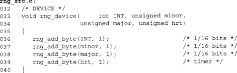
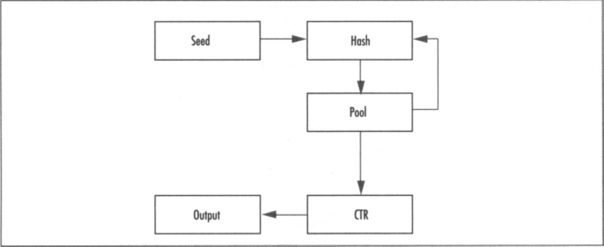
Essentially, the design hashes entropy along with the existing pool; this pool is then used a symmetric key for a cipher running in CTR mode (see Chapter 4, “Advanced Encryption Standard”). The cipher running in CTR mode and produces the PRNG output fairly efficiently. The actual design for Yarrow specifies how and when reseeding should be issued, how to gather entropy, and so on. For our purposes, we are using it as a PRNG so we do not care where the seed comes from. That is, you should be able to assume the seed has enough entropy to address your threat model.
Readers are encouraged to read the design paper “Yarrow-160: Notes on the Design and Analysis of the Yarrow Cryptographic Pseudorandom Number Generator” by John Kelsey, Bruce Schneier, and Niels Ferguson to get the exact details, as our description here is rather simplistic.
Design
From the block diagram in Figures 3.4 and 3.5, we see that the existing pool and seed are hashed together to form the new pool (or state). The use of the hash avoids backtracking attacks. Suppose the hash of the seed data was simply XOR’ed into the pool; if an attacker knows the pool and can guess the seed data being fed to it, he can backtrack the state.
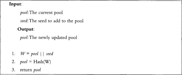
The hash of both pieces also helps prevent degradation where the existing entropy pool is used far too long. That is, while hashing the pool does not increase the entropy, it does change the key the CTR block uses. Even though the keys would be related (by the hash), it would be infeasible to exploit such a relationship. The CTR block need not refer to a cipher either; it could be a hash in CTR mode. For performance reasons, it is better to use a block cipher for the CTR block.
In the original Yarrow specification, the design called for the SHA-1 hash function and Blowfish block cipher (or only a hash). While these are not bad choices, today it is better to choose SHA-256 and AES, as they are more modern, more efficient, and part of various standards including the FIPS series. In this algorithm (Figure 3.6) we use the pool as a symmetric key and then proceed to CTR encrypt a zero string to produce output.
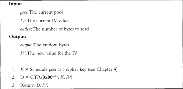
The notation 0x00outlen indicates a string of length outlen bytes of all zeroes. In step 2, we invoke the CTR routine for our cipher, which has not been defined yet. The parameters are <plaintext, key, IV>, where the IV is initially zeroed and then preserved through every call to the reseed and generate functions. Replaying the IV for the same key is dangerous, which is why it is important to keep updating it. The random bytes are in the string D, which is the output of encrypting the zero string with the CTR block.
Reseeding
The original Yarrow specification called for system-wide integration with entropy sources to feed the Yarrow PRNG. While not a bad idea, it is not the strong suit of the Yarrow design. As we shall see in the discussion of Fortuna, there are better ways to gather entropy from system events.
For most cryptographic tasks that are short lived, it is safe to seed Yarrow once from a system RNG. A safe practical limit is to use a single seed for at most one hour, or for no more than 2(w/4) CTR blocks where w is the bit size of the cipher (e.g., w = 128 for AES). For AES, this limit would be 232 blocks, or 64 gigabytes of PRNG output. (On AMD Opteron processors, it is possible to generate 232 outputs in far less than one hour (would take roughly 500 seconds). So, this limitation is actually of practical importance and should be kept in mind.)
Technically, the limit for CTR mode is dictated by the birthday paradox and would be 2(w/2); using 2(w/4) ensures that no distinguisher on the underlying cipher is likely to be possible. Currently, there are no attacks on the full AES faster than brute force; however, that can change, and if it does, it will probably not be a trivial break. Limiting ourselves to a smaller output run will prevent this from being a problem effectively indefinitely.
These guidelines are merely suggestions. The secure limits depend on your threat model. In some systems, you may want to limit a seed’s use to mere minutes or to single outputs. In particular, after generating long-term credentials such as public key certificates, it is best to invalidate the current PRNG state and reseed immediately.
Statefulness
The pool and the current CTR counter value can dictate the entire Yarrowstate (see Chapter 4). In some platforms, such as embedded platforms, we may wish to save the state, or at least preserve the entropy it contains for a future run.
This can be a thorny issue depending on if there are other users on the system who could be able to read system files. The typical solution, as used by most Linux distributions, is to output random data from the system RNG to a file and then read it at startup. This is certainly a valid solution for this problem. Another would be to hash the current pool and store that instead. Hashing the pool itself directly captures any entropy in the pool.
From a security point of view, both techniques are equally valid. The remaining threat comes from an attacker who has read the seed file. Therefore, it is important to always introduce a fresh seed whenever possible upon startup. The usefulness of a seed file is for the occasions when local users either do not exist or cannot read the seed file. This allows the system to start with entropy in the PRNG state even if there are few or no events captured yet.
Pros and Cons
The Yarrow design is highly effective at turning a seed into a lengthy random looking string. It relies heavily on the one-wayness and collision resistance of the hash, and the behavior of the symmetric cipher as a proper pseudo-random permutation. Provided with a seed of sufficient entropy, it is entirely possible to use Yarrow for a lengthy run.
Yarrow is also easy to construct out of basic cryptographic primitives. This makes implementation errors less likely, and cuts down on code space and memory usage.
On the other hand, Yarrow has a very limited state, which always runs the risk of state discovery attacks. While they are not practical, it does run this theoretical risk. As such, it should be avoided for longer term or system-wide deployment.
Yarrow is well suited for many short-lived tasks in which a small amount of entropy is required. Such tasks could be things like command-line tools (e.g., GnuPG), network sensors, and small servers or clients (e.g., DSL router boxes).
Fortuna PRNG
The Fortuna design was proposed by Niels Ferguson and Bruce Schneier2 as effective an upgrade to the Yarrow design. It still uses the same CTR mechanism to produce output, but instead has more reseeding elements and a more complicated pooling system. (See Niels Ferguson and Bruce Schneier, Practical Cryptography, published by Wiley in 2003.)
Fortuna addresses the small PRNG state of Yarrow by having multiple pools and only using a selection of them to create the symmetric key used by the CTR block. It is more suited for long-lived tasks that have periodic re-seeding and need security against malleability and backtracking.
Design
The Fortuna design is characterized mostly by the number of entropy pools you want gathering entropy. The number depends on how many events and how frequently you plan to gather them, how long the application will run, and how much memory you have. A reasonable number of pools is anywhere between 4 and 32; the latter is the default for the Fortuna design.
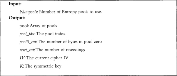
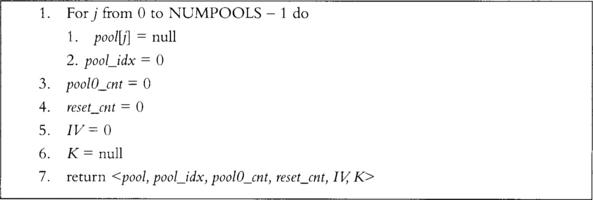
When the algorithm is started (Figure 3.7), all pools are effectively zeroed out and emptied. A pool counter, pool_idx, indicates which pool we are pointing at; pool0_cnt indicates the number of bytes added to the zero’th pool; and reset_cnt indicates the number of times the PRNG has been reseeded (reset the CTR key).
The pools are not actually buffers for data; in practice, they are implemented as hash states that accept data. We use hash states instead of buffers to allow large amounts of data to be added without wasting memory.
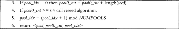
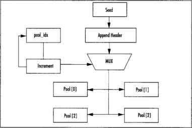
When entropy is added (Figures 3.8 and 3.9), it is prepended with a two-byte header that contains an ID byte and length byte. The ID byte is simply an identifier the developer chooses to separate between entropy sources. The length byte indicates the length in bytes of the entropy being added. The entropy is logically added to the pool_idx’th pool, which as we shall see amounts to adding it the hash of the pool. If we are adding to the zero’th pool, we increment pool0_cnt by the number of bytes added. Next, we increment pool_idx and wrap back to zero when needed. If during the addition of entropy to the zero’th pool it exceeds a minimal size (say 64 bytes), the reseed algorithm should be called.

Note that in our figures we use a system with four pools. Fortuna is by no means limited to that. We chose four to make the diagrams smaller.
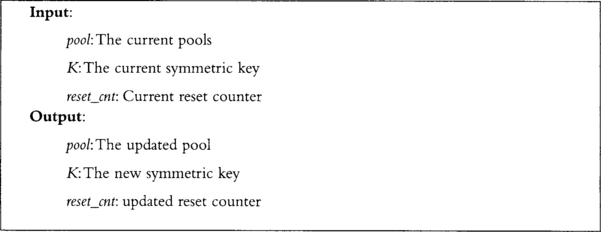
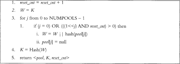
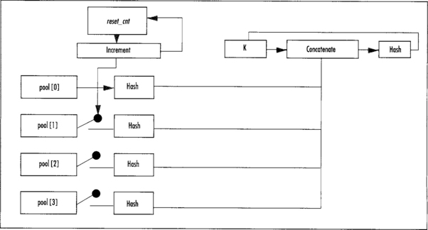
Reseeding will take entropy from select pools and turn it into a symmetric key (K) for the cipher to use to produce output (Figures 3.10 and 3.11). First, the reset_cnt counter is incremented. The value of reset_cnt is interpreted as a bit mask; that is, if bit x is set, pool x will be used during this algorithm. All selected pools are hashed, all the hashes are concatenated to the existing symmetric key (in order from first to last), and the hash of the string of hashes is used as the symmetric key. All selected pools are emptied and reset to zero. The zero’th pool is always selected.
Extracting entropy from Fortuna is relatively straightforward. First, if a given amount of time has elapsed or a number of reads has occurred, the reseed function is called. Typically, as a system-wide PRNG the time delay should be short; for example, every 10 seconds. If a timer isn’t available or this isn’t running as a daemon, you could use every 10 calls to the function.
After the reseeding has been handled, the cipher in CTR mode, can generate as many bytes as the caller requests. The IV for the cipher is initially zeroed when the algorithm starts, and then left running throughout the life of the algorithm. The counter is handled in a little-endian fashion incremented from byte 0 to byte 15, respectively.
After all the output has been generated, the cipher is clocked twice to re-key itself for the next usage. In the design of Fortuna they use an AES candidate cipher; we can just use AES for this (Fortuna was described before the AES algorithm was decided upon). Two clocks produce 256 bits, which is the maximally allowed key size. The new key is then scheduled and used for future read operations.
Reseeding
Fortuna does not perform a reseed operation whenever entropy is being added. Instead, the data is simply concatenated to one of the pools (Figure 3.5) in a round-robin fashion. Fortuna is meant to gather entropy from pretty much any source just like our system RNG described in rng.c.
In systems in which interrupt latency is not a significant problem, Fortuna can easily take the place of a system RNG. In applications where there will be limited entropy additions (such as command-line tools), Fortuna breaks down to become Yarrow, minus the rekeying bit). For that reason alone, Fortuna is not meant for applications with short life spans.
A classic example of where Fortuna would be a cromulent choice is within an HTTP server. It gets a lot of events (requests), and the requests can take variable (uncertain) amounts of time to complete. Seeding Fortuna with these pieces of information, and from a system RNG occasionally, and other system resources, can produce a relatively efficient and very secure userspace PRNG.
Statefulness
The entire state of the Fortuna PRNG can be described by the current state of the pools, current symmetric key, and the various counters. In terms of what to save when shutting down it is more complicated than Yarrow.
Simply emitting a handful of bytes will not use the entropy in the later pools that have yet to be used. The simplest solution is to perform a reseeding with reset_cnt equal to the all ones pattern subtracted by one; all pools will get affected the symmetric key. Then, emit 32 bytes from the PRNG to the seed file.
If you have the space, storing the hash of each pool into the seed file will help preserve longevity of the PRNG when it is next loaded.
Pros and Cons
Fortuna is a good design for systems that have a long lifetime. It provides for forward secrecy after state discovery attacks by distributing the entropy over long bit extractions. It is based on well-thought-out design concepts, making its analysis a much easier process.
Fortuna is best suited for servers and daemon style applications where it is likely to gather many entropy events. By contrast, it is not well suited for short-lived applications. The design is more complicated than Yarrow, and for short-lived applications, it is totally unnecessary. The design also uses more memory in terms of data and code.
NIST Hash Based DRBG
The NIST Hash Based DRBG (deterministic random bit generator) is one of three newly proposed random functions under NIST SP 800-90. Here we are only talking about the Hash_DRBG algorithm described in section 10.1 of the specification. The PRNG has a set of parameters that define various variables within the algorithm (Table 3.1).

Design
The internal state of Hash_DRBG consists of:
![]() A value V of seedlen bits that is updated during each call to the DRBG.
A value V of seedlen bits that is updated during each call to the DRBG.
![]() A constant C of seedlen bits that depends on the seed.
A constant C of seedlen bits that depends on the seed.
![]() A counter reseed_counter that indicates the number of requests for pseudorandom bits since new entropy_input was obtained during instantiation or reseeding.
A counter reseed_counter that indicates the number of requests for pseudorandom bits since new entropy_input was obtained during instantiation or reseeding.
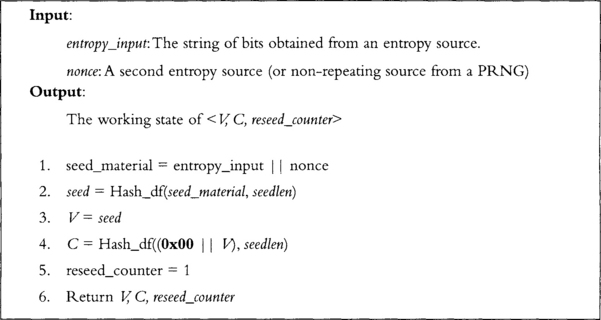
The PRNG is initialized through the Hash_DRBG instantiate process (section 10.1.1.2 of the specification).
This algorithm returns a working state the rest of the Hash_DRBG functions can work with (Figure 3.12). It relies on the function hash_df() (Figure 3.13), which we have yet to define. Before that, let’s examine the reseed algorithm.

This algorithm (Figure 3.14) takes new entropy and mixes it into the state of the DRBG. It accepts additional input in the form of application specific bits. It can be null (empty), and generally it is best to leave it that way. This algorithm is much like Yarrow in that it hashes the existing pool (V) in with the new entropy. The seed must be seedlen bits long to be technically following the specification. This alone can make the algorithm rather obtrusive to use.
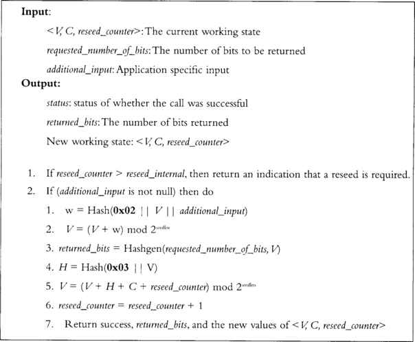
This function takes the working state and extracts a string of bits. It uses a hash function denoted by Hash() and a new function Hashgen(), which we have yet to present. Much like Fortuna, this algorithm modifies the pool (V) before returning (step 5). This is to prevent backtracking attacks.
This function performs a stretch of the input string to the desired number of bits of output (Figure 3.15). It is similar to algorithm Hashgen (Figure 3.16) and currently it is not obvious why both functions exist when they perform similar functions.
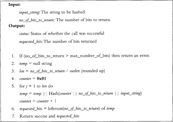
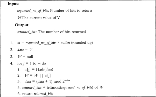
This function performs the stretching of the input seed for the generate function. It effectively is similar enough to Hash_df (Figure 3.15) to be confused with one another. The notable difference is that the counter is added to the seed instead of being concatenated with it.
Reseeding
Reseeding Hash_DRBG should follow similar rules as for Yarrow. Since there is only one pool, all sourced entropy is used immediately. This makes the long-term use of it less advisable over, say, Fortuna.
Statefulness
The state of this PRNG consists of the V, C, and reseed_counter variables. In this case, it is best to just generate a random string using the generate function and save that to your seedfile.
Pros and Cons
The Hash_DRBG function is certainly more complicated than Yarrow and less versatile than Fortuna. It addresses some concerns that Yarrow does not, such as state discovery attacks. However, it also is fairly rigid in terms of the lengths of inputs (e.g., seeds) and has several particularly useless duplications. We should note that NIST SP 800–90, at the time of writing, is still a draft and is likely to change.
On the positive side, the algorithm is more robust than Yarrow, and with some fine tuning and optimization, it could be made nearly as simple to describe and implement. This algorithm and the set of SP 800–90 are worth tracking. Unfortunately, at the time of this writing, the comment period for SP 800–90 is closed and no new drafts were available.
Putting It All Together
The first thing to tackle in designing a cryptosystem is to figure out if you need an RNG or merely a well-seeded PRNG for the generation of random bits. If you are making a completely self-contained product, you will definitely require an RNG. If your application is hosted on a platform such as Windows or Linux, a system RNG is the best choice for seeding an application PRNG.
Typically, an RNG is useful under two circumstances: lack of nonvolatile storage and the requirement for tight information theoretic properties. In circumstances where there is no proper nonvolatile storage, you cannot forward a seed from one runtime of the device (or application) to another. You could use what are known as fuse bits to get an initial state for the PRNG, but re-using it would result in an insecure process. In these situations, an RNG is required to at least seed the PRNG initially at every launch.
In other circumstances, an application will need to remove the assumption that the PRNG produces bits that are indistinguishable from truly random bits. For example, a certificate signing authority really ought to use an RNG (or several) as its source of random bits. Its task is far too important to assume that at some point the PRNG was well seeded.
Fuse Bits
Fuse bits are essentially a form of ROM that is generated after the masking stage of tape-out (tape-out is the name of the final stage of the design of an integrated circuit; the point at which the description of a circuit is sent for manufacture). Each instance of the circuit would have a unique random pattern of bits literally fused into themselves. These bits would serve as the initial state of the PRNG and allow traceability and diagnostics to be performed. The PRNG could be executed to determine correctness and a corresponding host device could generate the same bits (if need be).
Fuse bits are not modifiable. This means your device must never power off, or must have a form of nonvolatile storage where it can store updated copies of the PRNG state. There are ways to work around this limitation. For example, the fuse bits could be hashed with a real-time clock output to get a new PRNG working state. This would be insecure if the real-time clock cannot be trusted (e.g., rolled back to a previous time), but otherwise secure if it was left alone.
Use of PRNGs
For circumstances where an RNG is not a strict requirement, a PRNG may be a more suitable option. PRNGs are typically faster than RNGs, have lower latencies, and in most cases provide the same effective security as an RNG would provide.
The life of a PRNG within an application always begins with at least one reseed operation. On most platforms, a system-wide RNG is available. A short read of at least 256 bits provides enough seed material to start a PRNG in an unpredictable (from an adversary’s point of view) state.
Although you need at least one reseed operation, it is not inadvisable to reseed during the life of an application. In practice, even seeds of little to no entropy should be safe to feed to any secure PRNG reseed function. It is ideal to force a reseed after any event that has a long lifetime, such as the generation of user credentials.
When the application is finished with the cryptographic services it’s best to either save the state and/or wipe the state from memory. On platforms where an RNG is available, it does not always make sense to write to a seedfile—the exception being applications that need entropy prior to the RNG being available to produce output (during a boot up, for example). In this case, the seedfile should not contain the state of the PRNG verbatim; that is, do not write the state directly to the seedfile. Instead, it should either be the result of calling the PRNG’s generate function to emit 256 bits (or more) or be a one-way hash of the current state. This means that an attacker who can read the saved state still can’t go backward to recover previous outputs.
Do’s
![]() Do reseed at least once with at least 256 bits from an RNG you trust.
Do reseed at least once with at least 256 bits from an RNG you trust.
![]() Do reseed after generating long-term credentials.
Do reseed after generating long-term credentials.
Example Platforms
Desktop and Server platforms are often similar in their use of base components. Servers are usually differentiated by their higher specification and the fact they are typically multiway (e.g., multiprocessor). They tend to share the following components:
![]() High-resolution processor timers (e.g., RDTSC)
High-resolution processor timers (e.g., RDTSC)
![]() Sound codec (e.g., Intel HDA or AC′97 compatible)
Sound codec (e.g., Intel HDA or AC′97 compatible)
![]() USB, PS/2, serial and parallel ports
USB, PS/2, serial and parallel ports
![]() SATA, SCSI, and IDE ports (with respective storage devices attached)
SATA, SCSI, and IDE ports (with respective storage devices attached)
The load on most servers guarantees that a steady stream of storage and network interrupts is available for harvesting. Desktops typically will have enough storage interrupts to get an RNG going.
In circumstances where interrupts are sparse, the timer skew and ADC noise options are still open. It would be trivial as part of a boot script to capture one second of audio and feed it to the RNG. The supply of timer interrupts would ensure there is at least a gradual stream of entropy.
We mentioned the various ports readably available on any machine such as USB, PS/2, serial and parallel ports because various vendors sell RNG devices that feed the host random bits. One popular device is the SG100 (www.protego.se/sg100_en.htm) nine-pin serial port RNG. It uses the noise created by a diode at threshold. They also have a USB variant (www.protego.se/sg200_d.htm) for more modern systems. There are others, such as the RPG100B IC from FDK (www.fdk.co.jp/cyber-e/pi_ic_rpg100.htm), which is a small 32-pin chip that produces up to 250Kbit/sec of random data.
Seedfiles are often a requirement for these platforms, as immediately after boot there is usually not enough entropy to seed a PRNG. The seedfile must be either updated or removed during the shutdown process to avoid re-using the same seed. A safe way to proceed is to remove the seedfile upon boot; that way, if the machine crashes there is no way to reuse the seed.
Consoles
Most video game consoles are designed and produced well before security concerns are thought of. The Sony PS2 brought the broadband adapter without an RNG, which meant that most connections would likely be made in the clear. Similarly, the Sony PSP and Nintendo DS are network capable without any cryptographic facilities.
In these cases, it is easy to say, “just use an RNG,” except that you do not have one readily available. What you do have is a decent source of interrupts and interaction, and nonvolatile space to store seed data. Entropy on these platforms comes in the form of the user input, usually from a controller of some sort combined with timer data. The RNG presented earlier would be quick enough to minimize the performance impact of such operations. In the case of the Nintendo DS, a microphone is available that also can supply a decent amount of entropy from ADC noise.
For performance reasons, it is not ideal to leave the RNG running for the entire lifetime of the game. Users may tolerate some initial slowdown while the RNG gets fed, but will not tolerate slowdown during gameplay. In these cases, it is best to seed a PRNG with the RNG and use it for any entropy the game requires. Often, entropy is only required to establish connections, after which the cryptosystem is running and requires no further entropy.
Seed management is a bit tricky on these platforms. Ideally, you would like to save entropy for the next run, as the user would like to start playing quickly and ensure the transaction is secure. All popular consoles available as of June 2006 have the capability of storing data, whether an internal hard drive, an external flash memories, or internal to the game cartridge (like in the Nintendo DS cartridges). The trick with these platforms is to save a new seed when you have enough entropy and before the user randomly turns the power off. On most platforms, the power button is software driven and can signal an interrupt. However, we may have to deal with power outages or other shutdowns such as crashes.
In these cases, it is best to invalidate the seed after booting to avoid using it twice. As the program runs, the RNG will gather data, and as soon as enough entropy is available should initialize the PRNG. The PRNG generate function can then be used to generate a new seedfile.
Typically, data written locally is safe from prying eyes. That is, you can write the seed and then use it as your sole source of entropy in future runs. However, the entropy of the seed can degrade, and this process does not work for rentals (such as Nintendo DS games). It is always best to gather at least 256 bits of additional entropy in the RNG before seeding the PRNG and writing the new seedfile.
Network Appliances
Network appliances face the same battle as consoles. They usually do not have a lot of storage and are not in well-conditioned states upon first use. A typical network appliance could be something like a DSL router, probe, camera, or access devices (like RFID locks). They require cryptography to authenticate and encrypt data between some client or server and itself. For example, you may log in via SSL to your DSL router, your remote camera may SFTP files to your desktop, and your RFID door must authenticate an attempt with a central access control server.
These applications are better suited for hardware RNGs than software RNGs, as they are typically custom designs. It is much easier to design a diode RNG into the circuit than a complete finite state machine that requires a one-way hash function. Even worse, most network devices do not have enough interrupts to generate any measurable entropy.
The following Frequently Asked Questions, answered by the authors of this book, are designed to both measure your understanding of the concepts presented in this chapter and to assist you with real-life implementation of these concepts. To have your questions about this chapter answered by the author, browse to www.syngress.com/solutions and click on the “Ask the Author” form.
A: Entropy is the measure of uncertainty in an observable event, and is typically expressed in terms of bits since it is usually mapped on to binary decision graphs. For example, a perfect coin toss is said to have one bit of entropy since the outcome will be heads or tails with equal probability
A: An event is something the RNG or PRNG algorithm can observe, such as hardware interrupts. Data related to the event such as which event and when it occurred can be extracted for their entropy.
Q: Where do I find a standard RNG design?
A: Unfortunately, there is no (public) RNG design mandated by public governments. What they do standardize on are the RNG tests. Your design must pass them to be FIPS 140–2 certified. In fact, even this isn’t enough. To pass certification, it must test itself every time it is started. This is to ensure the hardware hasn’t failed.
A: Yes, RNG design is essentially science and guestimation. How many bits of entropy are there in your mouse movements? It’s hard to say exactly, which is why it is suggested to estimate conservatively.
Q: Why should I not just use an RNG all the time?
A: RNGs tend to be slower and block more often than PRNG algorithms (which rarely if ever use blocking). This means it is harder to use an RNG during the runtime of an application. For most purposes, the fact that the PRNG is guaranteed to return a result straight away is better.
Q: What is the practical significance between the short and long lifetime PRNGs?
A: Yarrow, at least as presented in this text, is safe to use for both short and long lifetimes provided it has been seeded frequently. Fortuna spreads its input entropy over a longer runtime, which makes it more suitable for longer run applications. In practice, however, provided the PRNG was well seeded, and you do not generate large amounts of bits, the output would be safe to use.
Q: What other PRNG standards are there?
A: NIST SP 800–90 specifies a cipher, HMAC and Elliptic Curve based PRNGs. ANSI X9.31 specifies a triple-DES bit generator, which has since been amended to include AES support.
Q: Is there anything that’s truly random?
A: Yes, the standard model of quantum mechanics allows for processes that are truly random. The most commonly cited example of this is radioactive decay of elements.
It is possible to extract a great deal of entropy from radioactive decay by hooking up a Geiger-counter to a computer. Entropy is extracted by measuring the length of time between pairs of decays. If the time between the first pair of decays is shorter than the second pair, record a zero. If the time between the second pair of decays is longer than the second pair, record a one. Random bits generated in this way have an entropy very close to 1-bit per bit.
It is highly unlikely that there is an underlying pattern to radioactive decay. If there was, Quantum Mechanics as we know it would not be possible. Weigh this against the fact that Quantum Mechanics has been verified to a factor of one in many million. If one of the fundamental tenants of Quantum Mechanics were wrong, it would be deeply surprising.
Aside from quantum mechanics, it is quite possible to have entropy in systems that are deterministic. Consider a particle traveling at a speed exactly equal to the square root of five meters per second. We can never compute all the decimal places of the square root of five, because it is irrational. That means that for any finite expansion, there is always a small degree of entropy in the value. (Of course, we can always do more calculations to obtain the next decimal place, so such expansions are not suitable for cryptography.)