
11.2.1 Time Warping
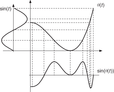
Suppose that we want to change the shape of a periodic waveform s(t) by moving the amplitude values attained by the signal to other time instants. One can achieve this by plotting the signal on an elastic sheet and by stretching and/or compressing the sheet at different points along its horizontal direction. The waveshape appears as if the original time axis had been deformed. Instants of time that were equidistant now have a different time distribution. This deformation of the time axis called time warping is characterized by a warping map θ(t), mapping points of the original t-axis onto points of the transformed axis. An example of time warping a sinewave is shown in Figure 11.1. The figure is obtained by plotting the original signal along the ordinates and transforming time instants into new time instants via the warping map, obtaining the signal plotted along the abscissa axis. Notice that to one point in the original signal there can correspond more points in the warped signal. These points are obtained by joining time instants of the original signal to points on the warping characteristic θ(t) using horizontal lines. The corresponding warped time instants are the value(s) of the abscissa corresponding to these intersection point(s). The time-warped signal is obtained by plotting the corresponding amplitude values at the new time instants along the abscissa. In this example the signal sin(θ(t)) may be interpreted as a phase modulation of the original sinewave. Time warping a signal composed of a superposition of sinewaves is equivalent to phase modulating each of the component sinewaves and adding them together. By time warping we alter not only the waveshape, but also the period of the signal. Clearly, the map is an effective modulo of the period of the signal, that is, the map θ(t) and the map
![]()
where ![]() denotes the remainder of the integer division of x by T, have the same net effect on a T-periodic signal. More generally, we can time warp an arbitrary, aperiodic signal s(t) via an arbitrary map, obtaining a signal
denotes the remainder of the integer division of x by T, have the same net effect on a T-periodic signal. More generally, we can time warp an arbitrary, aperiodic signal s(t) via an arbitrary map, obtaining a signal
![]()
whose waveshape and envelope may be completely different from the starting signal. If the map is invertible, i.e., one-to-one, then
![]()
that is, at time τ = θ−1(t) the time-warped signal attains the same amplitude value as that attained by the starting signal at time t.
Figure 11.1 Time warping a sinewave by means of an arbitrary map θ(t).
Time-warping transformations are useful for musical applications, e.g., for morphing a sound into a new one in the time domain.
11.2.2 Frequency Warping
Frequency warping is the frequency-domain counterpart of time warping. Given a signal whose discrete-time Fourier transform (DTFT) is S(ω), we form the signal sfw(t) whose DTFT is
![]()
That is, the frequency spectrum of the frequency-warped signal agrees with that of the starting signal at frequencies that are displaced by the map θ(ω). If the map is invertible, then
![]()
The frequency-warped signal is obtained by computing the inverse DTFT of the warped frequency spectrum. In order to obtain a real warped signal from a real signal, the warping map must have odd parity, i.e.,
![]()
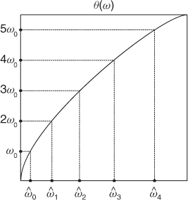
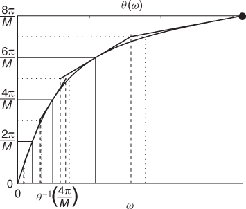
In order to illustrate the features of frequency warping, consider a periodic signal s(t) whose frequency spectrum peaks at integer multiples of the fundamental frequency ω0. The frequency spectrum of the warped signal will peak at frequencies
![]()
The situation is illustrated in Figure 11.2, where the original harmonic frequencies are represented by dots along the ordinate axis. The warped frequencies are obtained by drawing horizontal lines from the original set of frequencies to the graph of θ(ω) and by reading the corresponding values of the abscissa. As a result, harmonically related partials are mapped onto non-harmonically related ones. Furthermore, if the frequency-warping map is not monotonically increasing, one obtains effects analogous to the foldover of frequencies. This is similar to that which is obtained from a phase vocoder in which the frequency bands are scrambled in the synthesis of the signal. However, the resolution and flexibility of the frequency-warping method are generally much higher than that of the scrambled phase vocoder.
Figure 11.2 Frequency warping of a periodic signal: transformation of the harmonics into inharmonic partials.
Energy Preservation and Unitary Frequency Warping
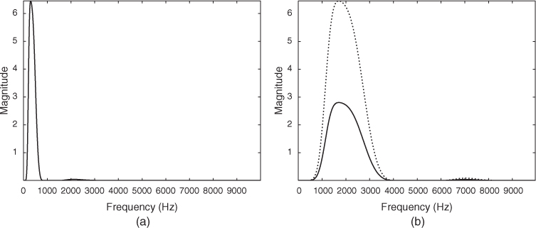
By frequency warping a signal one dilates or shrinks portions of its frequency spectrum. As a result, the areas under the spectral characteristics are affected. Perceptually this results in an amplification of certain bands and an attenuation of other bands. This is depicted in Figure 11.3 where the original narrow band spectrum of Figure 11.3(a) is dilated, obtaining the dotted curve shown in Figure 11.3(b). In order to circumvent this problem, which causes an alteration of the relative energy levels of the spectrum, one should perform an equalization aimed at reducing the amplitude of dilated portions and increasing that of shrunk portions of the spectrum. Mathematically this is simply achieved, in the case where the warping map is increasing, by scaling the magnitude square of the DTFT of the warped signal by the derivative of the warping map. In fact, the energy in an arbitrary band [ω0, ω1] is
![]()
By the simple change of variable ω = θ(Ω) in the last integral we obtain

where
is the DTFT of the scaled frequency warped signal. Equation (11.1) states the energy preservation property of the scaled warped signal in any band of the spectrum: the energy in any band [ω0, ω1] of the original signal equals the energy of the warped signal in the warped band [θ−1(ω0), θ−1(ω1)]. Thus, the scaled frequency warping is a unitary operation on signals.
Figure 11.3 Frequency warping a narrow-band signal: (a) original frequency spectrum; (b) frequency-warped spectrum (dotted line) and scaled frequency-warped spectrum (solid line).
11.2.3 Algorithms for Warping
In Sections 11.2.1 and 11.2.2 we explored basic methods for time warping in the time domain and frequency warping in the frequency domain, respectively. However, one can derive time- and frequency-warping algorithms in crossed domains. It is easy to realize that time and frequency warping are dual operations. Once a time-domain algorithm for frequency warping is determined, then a frequency-domain algorithm for time warping will work the same way. This section contains an overview of techniques for computing frequency warping. The same techniques can be used for time warping in the dual domain. We start from the basic maps using the Fourier transform and end up with time-varying warping using allpass chains in dispersive delay lines.
Frequency Warping by Means of FFT
A simple way to implement the frequency-warping operation on finite length discrete-time signals is via the FFT algorithm. Let
denote the DFT of a length N signal s(n). Consider a map ![]() mapping the interval [−π, π] onto itself and extend
mapping the interval [−π, π] onto itself and extend ![]() outside this interval by letting
outside this interval by letting
![]()
The last requirement is necessary in order to guarantee that the warped discrete-time signal has a 2π-periodic Fourier transform
![]()
i.e., Sfw(ω) is the Fourier transform of a discrete-time signal. In order to obtain the frequency-warped signal we would need to compute ![]() and then perform the inverse Fourier transform. However, from the DFT we only know
and then perform the inverse Fourier transform. However, from the DFT we only know ![]() at integer multiples of
at integer multiples of ![]() The map
The map ![]() is arbitrary and
is arbitrary and ![]() is not necessarily a multiple of
is not necessarily a multiple of ![]() However, we may approximate
However, we may approximate ![]() with the nearest integer multiple of
with the nearest integer multiple of ![]() i.e., we can define the quantized map
i.e., we can define the quantized map
![]()
The values ![]() are known from the DFT of the signal and we can compute the approximated frequency-warped signal by means of the inverse DFT:
are known from the DFT of the signal and we can compute the approximated frequency-warped signal by means of the inverse DFT:
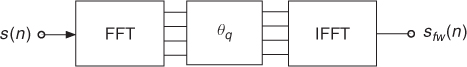
The diagram of the frequency-warping algorithm via FFT is shown in Figure 11.4. If the warping map is an increasing function, one can introduce the equalization factor as in (11.2) simply by multiplying ![]() by the factor
by the factor ![]() before processing with the IFFT block. The FFT algorithm for warping is rather efficient, with a complexity proportional to NlogN. However, it has some drawbacks. The quantization of the map introduces distortion in the desired frequency spectrum, given by repetitions of the same value in phase and magnitude at near frequencies. These sum almost coherently and are perceived as beating components that have a slow amplitude decay. In frequency-warping signals one must pay attention to the fact that the warped version of a finite-length signal is not necessarily finite length. In the FFT-warping algorithm, components that should lie outside the analysis interval are folded back into it causing some echo artifacts. Furthermore, even if the original warping map is one-to-one, the quantized map is not and the warping effect cannot be undone without losses. The influence of the artifacts introduced by the FFT-warping algorithms may be reduced by zero-padding the original signal in order to obtain a larger value of N and, at the same time, a smaller quantization step for θ, at the expense of an increased computational cost.
before processing with the IFFT block. The FFT algorithm for warping is rather efficient, with a complexity proportional to NlogN. However, it has some drawbacks. The quantization of the map introduces distortion in the desired frequency spectrum, given by repetitions of the same value in phase and magnitude at near frequencies. These sum almost coherently and are perceived as beating components that have a slow amplitude decay. In frequency-warping signals one must pay attention to the fact that the warped version of a finite-length signal is not necessarily finite length. In the FFT-warping algorithm, components that should lie outside the analysis interval are folded back into it causing some echo artifacts. Furthermore, even if the original warping map is one-to-one, the quantized map is not and the warping effect cannot be undone without losses. The influence of the artifacts introduced by the FFT-warping algorithms may be reduced by zero-padding the original signal in order to obtain a larger value of N and, at the same time, a smaller quantization step for θ, at the expense of an increased computational cost.
Figure 11.4 Frequency warping by means of FFT: schematic diagram.
Dispersive Delay Lines
In order to derive alternate algorithms for frequency warping [Bro65, OJ72], consider the DTFT (11.2) of the scaled frequency-warped version of a causal signal s(n),
The last formula is obtained by considering the DTFT of the signal s(n), replacing ω with θ(ω) and multiplying by ![]() . The warped signal
. The warped signal ![]() is obtained from the inverse DTFT of
is obtained from the inverse DTFT of ![]() :
:
Defining the sequences λn(k) as follows,
we can put (11.4) in the form
If we find a way of generating the sequences λn(k), then we have a new algorithm for frequency warping, which consists of multiplying these sequences by the signal samples and adding the result. From (11.5) we have an easy way for accomplishing this since
11.7 ![]()
with
![]()
Notice that the term ![]() has magnitude 1 and corresponds to an allpass filter. The sequence λ0(k) may be generated as the impulse response of the filter
has magnitude 1 and corresponds to an allpass filter. The sequence λ0(k) may be generated as the impulse response of the filter ![]() The sequence λn(k) is obtained by filtering λn−1(k) through the allpass filter
The sequence λn(k) is obtained by filtering λn−1(k) through the allpass filter ![]() This can be realized in the structure of Figure 11.5 for computing the sequences λn(k) as the impulse responses of a chain of filters. In order to perform warping it suffices to multiply each of the outputs by the corresponding signal sample and sum these terms together. The structure is essentially a delay line in which the elementary delays are replaced by allpass filters. Each of these filters introduces a frequency dependent group delay
This can be realized in the structure of Figure 11.5 for computing the sequences λn(k) as the impulse responses of a chain of filters. In order to perform warping it suffices to multiply each of the outputs by the corresponding signal sample and sum these terms together. The structure is essentially a delay line in which the elementary delays are replaced by allpass filters. Each of these filters introduces a frequency dependent group delay
![]()
The result is reminiscent of propagation of light in dispersive media where speed depends on frequency. For this reason this structure is called a dispersive delay line. What happens if we input a generic signal y(k) to the dispersive delay line? The outputs ![]() are computed as the convolution of the input signal by the sequences λn(k),
are computed as the convolution of the input signal by the sequences λn(k),
![]()
As a special case, for k = 0 and choosing as input the signal s(k) = y(−k), which is the time-reversed version of y(k), we obtain
![]()
The last equation should be compared with (11.6) to notice that the summation is now over the argument λn(r). However, we can define the transposed sequences
![]()
and write
From (11.5) we have
Suppose that the map θ(ω) has odd parity, is increasing and maps π onto π. Then we can perform in (11.9) the same change of variable Ω = θ(ω) as in (11.1) to obtain
![]()
As a result,
![]()
hence the transposed sequences ![]() have the same form as the sequences λr(n) except that they are based on the inverse map θ−1(ω). Consequently, (11.8) is a formula for unwarping the signal. Furthermore, by exchanging the roles of θ(ω) and θ−1(ω), (11.8) is also a valid algorithm for warping. The corresponding structure is shown in Figure 11.6. The input signal is time reversed, then fed to the
have the same form as the sequences λr(n) except that they are based on the inverse map θ−1(ω). Consequently, (11.8) is a formula for unwarping the signal. Furthermore, by exchanging the roles of θ(ω) and θ−1(ω), (11.8) is also a valid algorithm for warping. The corresponding structure is shown in Figure 11.6. The input signal is time reversed, then fed to the ![]() filter and to the dispersive delay line. The output of each filter is collected at time k = 0 by means of switches closing at that instant to form the scaled frequency-warped sequence
filter and to the dispersive delay line. The output of each filter is collected at time k = 0 by means of switches closing at that instant to form the scaled frequency-warped sequence ![]() . The structures in Figures 11.5 and 11.6 still present some computational problems. In general, the transfer functions involved are not rational. Furthermore, an infinite number of filters is needed for computing the transform. One can show that the only one-to-one map implementable by a rational transfer function is given by the phase of the first-order allpass filter
. The structures in Figures 11.5 and 11.6 still present some computational problems. In general, the transfer functions involved are not rational. Furthermore, an infinite number of filters is needed for computing the transform. One can show that the only one-to-one map implementable by a rational transfer function is given by the phase of the first-order allpass filter
where −1 < b < 1. By varying the real parameter b in the allowed range, one obtains the family of Laguerre curves shown in Figure 11.7. The curves with a negative value of the parameter are the inverses of those with a positive value, i.e., the inverse mapping θ−1(ω) corresponds to a sign reversal of the parameter. One can show that for causal signals the derivative ![]() can be replaced by the filter
can be replaced by the filter
![]()
The structure in Figure 11.6 includes a time-reversal block and switches closing at time zero. It is clear that for a finite-length N signal one can equivalently form the signal s(N − n) and close the switches at time k = N. Furthermore, by inspection of the structure, the required number M of allpass filters is approximately given by N times the maximum group delay, i.e.,
![]()
A larger number of sections would contribute little or nothing to the output signal.
Figure 11.5 Dispersive delay line for generating the sequences λn(k).
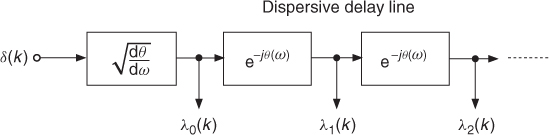
Figure 11.6 Computational structure for frequency warping.
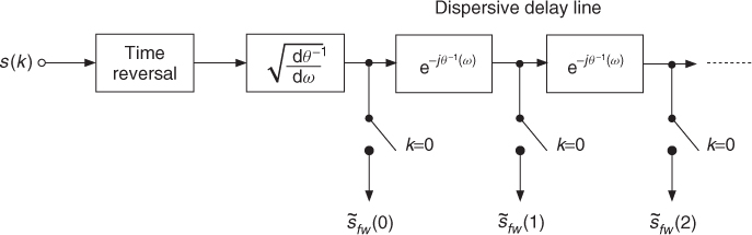
Figure 11.7 The family of Laguerre warping maps.

The main advantage of the time-domain algorithm for warping is that the family of warping curves is smooth and does not introduce artifacts, as opposed to the FFT-based algorithm illustrated in the above. Furthermore, the effect can be undone and structures for unwarping signals are obtained by the identical structure for warping provided that we reverse the sign of the parameter. In fact, the frequency-warping algorithm corresponds to the computation of an expansion over an orthogonal basis, giving rise to the Laguerre transform. Next we provide a simple MATLAB® function implementing the structure of Figure 11.6. The following M-file 11.1 gives a simple implementation of the Laguerre transform.
M-file 11.1 (lagt.m)
function y=lagt(x,b,M)
% Author: G. Evangelista
% computes M terms of the Laguerre transform y of the input x
% with Laguerre parameter b
N=length(x);
x=x(N:-1:1); % time reverse input
% filter by normalizing filter lambda_0
yy=filter(sqrt(1-b∧2),[1,b],x);
y(1)=yy(N); % retain the last sample only
for k=2:M
% filter the previous output by allpass
yy=filter([b,1],[1,b],yy);
y(k)=yy(N); % retain the last sample only
end
11.2.4 Short-time Warping and Real-time Implementation
The frequency-warping algorithm based on the Laguerre transform illustrated in Section 11.2.3 is not ideally suited to real-time implementation. Besides the computational cost, which is of the order of N2, each output sample depends on every input sample. Another drawback is that with a long signal the frequency-dependent delays cumulate to introduce large delay differences between high and low frequencies. As a result, the time organization of the input signal is destroyed by frequency warping. This can also be seen from the computational structure in Figure 11.6, where subsignals pertaining to different frequency regions of the spectrum travel with different speeds along the dispersive delay line. At sampling time some of these signals have reached the end of the line, whilst other are left behind. For example, consider the Laguerre transform of a signal s(n) windowed by a length N window h(n) shifted on the interval rM, ..., rM + N − 1. According to (11.6) we obtain
where
![]()
The DTFT of (11.11) yields
From this we can see that the spectral contribution of the signal supported on rM, ..., rM + N − 1 is delayed, in the warped signal, by the term ![]() , which introduces a largely dispersed group delay MτG(ω). Approximations of the warping algorithm are possible in which windowing is applied in order to compute a short-time Laguerre transform (STLT) and, at the same time, large frequency-dependent delay terms are replaced by constant delays. In order to derive the STLT algorithm, consider a window w(n) satisfying the perfect overlap-add condition
, which introduces a largely dispersed group delay MτG(ω). Approximations of the warping algorithm are possible in which windowing is applied in order to compute a short-time Laguerre transform (STLT) and, at the same time, large frequency-dependent delay terms are replaced by constant delays. In order to derive the STLT algorithm, consider a window w(n) satisfying the perfect overlap-add condition
where L ≤ N is an integer. This condition says that the superposition of shifted windows adds up to one. If ![]() denotes the Laguerre transform (11.6) of the signal s(n), then we have identically,
denotes the Laguerre transform (11.6) of the signal s(n), then we have identically,
By taking the DTFT of both sides of (11.14) one can show that
On the other hand, from (11.12) a delay compensated version of ![]() is
is
which is the DTFT of the sequence
11.17 
This equation defines the short-time Laguerre transform (STLT) of the signal s(n). In order to select the proper integer M we need to study the term X(r)(θ(ω)). One can show that
We would like to approximate the integral in (11.15) by Λ0(ω)X(r)(θ(ω)). Suppose that H(ω) is an unwarped version of W(ω), i.e., that
By performing in (11.18) the change of variable Ω = θ(ω) + θ(α − ω) we obtain
Since W(ω) is a lowpass function, only the terms for α ≈ ω contribute to the last integral. Therefore, from (11.16) and (11.20) we conclude that the superposition of delay-compensated versions of ![]() can be approximated as follows,
can be approximated as follows,

Equation (11.21) should be compared with (11.15). A linear approximation of θ(α) is
One can show that this is a fairly good approximation for ![]() In this frequency range, if we select
In this frequency range, if we select
then
![]()
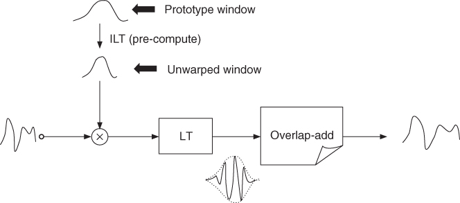
i.e., the overlap-add of STLT components well approximates the Laguerre transform. In other words, an approximate scheme for computing the Laguerre transform consists of taking the Laguerre transform of overlapping signal frames windowed by the unwarped window h(n) and overlap-adding the result, as shown in Figure 11.9. This method allows for a real-time implementation of frequency warping via the Laguerre transform. It relies on the linear approximation (11.22) of the phase of the allpass, valid for the low-frequency range. An important issue is the choice of the window w(n). Many classical windows, e.g., rectangular, triangular, etc., satisfy condition (11.13). However, (11.21) is a close approximation of the Laguerre transform only if the window sidelobes are sufficiently attenuated. Furthermore, the unwarped version (11.19) of the window can be computed via a Laguerre transform with the normalizing filter ![]() removed. In principle h(n) has infinite length. However, the inverse Laguerre transform of a lowpass window w(n) has essential length
removed. In principle h(n) has infinite length. However, the inverse Laguerre transform of a lowpass window w(n) has essential length
![]()
In order to avoid artifacts in the multiplication of the signal by the window, we are interested in windows whose Laguerre transform essentially is a dilated or stretched version of the window itself. This property turns out to be approximately well satisfied by the Hanning window
The choice of the length Nw is arbitrary. Furthermore, the Hanning window satisfies (11.13) for any L integer submultiple of Nw. Long windows tend to better approximate pure frequency warping. However, both response time and computational complexity increase with the length of the window. Moreover, the time-organization destruction effect is more audible using extremely long windows. The integer L controls the overlap Nw − L of the output warped frames. When warping with a positive value of the parameter b one should select a considerable overlap, e.g., Nw = 5L, in order to avoid amplitude distortion of the high-frequency components, which, in this case, are more concentrated in the Laguerre domain, as shown in Figure 11.8. Finally, the integer M fixing the input frames overlap is obtained by rounding the right-hand side of (11.23). Next we provide a simple M-file 11.2 implementing frequency warping by means of STLT overlap-add. The function gives a simple implementation of frequency warping via short-time Laguerre transform.1
M-file 11.2 winlagt.m
function sfw=winlagt(s,b,Nw,L)
% Author: G. Evangelista
% Frequency warping via STLT of the signal s with parameter b,
% output window length Nw and time-shift L
w=L*(1-cos(2*pi*(0:Nw-1)/Nw))/Nw; % normalized Hanning window
N=ceil(Nw*(1-b)/(1+b)); % length of unwarped window h
M=round(L*(1-b)/(1+b)); % time-domain window shift
h=lagtun(w,-b,N); h=h(:) % unwarped window
Ls=length(s); % pad signal with zeros
K=ceil((Ls-N)/M); % to fit an entire number
s=s(:); s=[s ; zeros(N+Kast M-Ls,1)]; % of windows
Ti=1; To=1; % initialize I/O pointers
Q=ceil(N*(1+abs(b))/(1-abs(b))); % length of Laguerre transform
sfw=zeros(Q,1); % initialize output signal
for k=1:K
yy=lagt(s(Ti:Ti+N-1).*h,b,Q); % Short-time Laguerre transf.
sfw(To:end)=sfw(To:end)+yy; % overlap-add STLT
Ti=Ti+M;To=To+L; % advance I/O signal pointers
sfw=[sfw; zeros(L,1)]; % zero pad for overlap-add
end
Figure 11.8 Short-time warping: different length of warped signals from low to high frequencies (top to bottom).
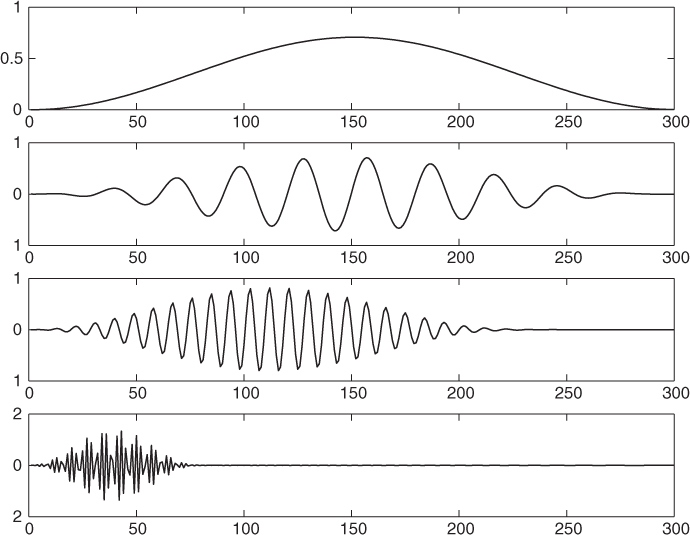
Figure 11.9 Block diagram of the approximate algorithm for frequency warping via overlap-add of the STLT components. The block LT denotes the Laguerre transform and ILT its inverse.
11.2.5 Vocoder-based Approximation of Frequency Warping
A major drawback of the short-time Laguerre-transform-based algorithm for warping described in Section 11.2.4 is that the warping map approximation (11.22) is only valid in the low-frequency range. This results in a choice of window length (11.23) that is satisfactory only in this range, generating artifacts for wideband signals. Moreover, the warping map θ(ω) is still constrained to follow one of the Laguerre curves in Figure 11.7.
An alternate approximate algorithm for frequency warping [EC07] can be derived from the STFT based time-frequency representation of the discrete time signal s(n),
where
11.25 ![]()
for q = 0, 1, …, M − 1 and r ∈ Z, are overlapping time-shifted and frequency-modulated windows and
are the STFT coefficients of the signal. The integer M controls the frequency resolution and is here constrained to an integer multiple M = KN of the time-shift integer N, for some integer K. If the window g has finite length M, then the factor K determines the number of windows that have non-zero overlap in each length N segment. Intuitively, each narrow-band component of the time-frequency representation intercepts only a small portion of the warping map θ, which makes a local linear approximation possible.
The analysis and synthesis real windows g(n) in (11.26) and (11.24) are identical as we assume that
11.27 ![]()
for perfect reconstruction. For our purposes, g(n) can be identified with the sine window
11.28 ![]()
in which case the following Parseval relationship holds true,
11.29 
Taking the DTFT of both sides of (11.24) yields
where
11.31 ![]()
As a result, the DTFT of the warped signal Sfw(ω) = S(θ(ω)) can be obtained from (11.30) by replacing the DTFT of the shifted-modulated windows Gq,r(ω) with the warped windows
Since the window is a low pass function, the warped windows (11.32) are essentially non-zero only for ω in the neighborhood of the roots of the equation ![]() . If the map θ is invertible, a first order Taylor series approximation about the unique roots
. If the map θ is invertible, a first order Taylor series approximation about the unique roots ![]() is then justified:
is then justified:
where
11.34 
Considering (11.33) for each synthesis band results in the locally linear approximation of the warping map shown in Figure 11.10.
Figure 11.10 Locally linear approximation of warping map: center bands (solid lines) and band edges (dotted lines).
In the same approximation we have
11.35 ![]()
Like several other windows, the sine window g(n) is obtained by sampling a continuous time function g(a)(t), so that g(n) = g(a)(n). In that case, one can show [EC07] that
which is a scaled, shifted and modulated version of the original window. For a unitary warping operation (see Section 11.2.2) the window (11.36) must be further multiplied by a factor ![]() , which is the square root of the derivative of the map evaluated at the point ωq.
, which is the square root of the derivative of the map evaluated at the point ωq.
Since the shift factor βqN is not necessarily an integer, the computation is greatly simplified if βqN is rounded to the nearest integer Nq. The resulting quantization error of the time-shift steps is negligible for sufficiently large N. Similarly, the window length βqM = βqKN can be rounded to the integer Mq = KNq. In this case, the approximated computation of frequency warping from the STFT Sq, r of the signal s(n) can be performed by means of the multirate filter bank shown in Figure 11.11, where
11.37 ![]()
with phase factors γq = Nqωq.
Figure 11.11 Synthesis filter bank structure for computing approximate frequency warping from STFT analysis coefficients.
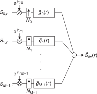
The modulating frequencies of the impulse responses of the various channels of the filter bank are not harmonically related and the window length is channel dependent. Therefore, while the analysis coefficients can be obtained by frame-by-frame FFT, the approximate warping synthesis structure cannot be implemented in an efficient FFT-based computational scheme. In the operation count per number of samples, the synthesis filter bank has linear complexity. If the signal is real and if the warping map has odd symmetry, then only the first half of the complex filter-bank sections need to be computed, the output being formed by taking the real part.
With the given time-frequency approximate warping algorithm, real-time operation is only possible if Nq ≥ N for any q. This constraint is satisfied if θ′(ω) ≥ 1 for any ω. In fact, in the multirate structure in Figure 11.11 each channel operates at a different rate regulated by the upsampling factor Nq. When Nq < N the synthesis structure produces fewer samples than those required by the STFT analysis block. In this case, the output lags behind the input and real-time operation is ruled out. In synthesis applications the map and the input pitch can both be suitably scaled to guarantee real-time operation. In audio effects applications, in order to compute warping in real-time, interpolation or prediction of the STFT data must be introduced in those channels where the warping map has θ′(ω) < 1, similarly to that often introduced in real-time pitch-shifters when the pitch is shifted upwards.
The artifacts introduced by the vocoder approximation of frequency warping are much less severe than the ones introduced with short-time Laguerre transform, both numerically and perceptually, as measured with PEAQ quality index. The main problems arise from the quantization of time-shift step and window length, especially in conjunction with flatter portions of the warping map (small derivative). These problems are mitigated by using proportionally larger values of M and N. Increasing the overlap does not improve quality.
11.2.6 Time-varying Frequency Warping
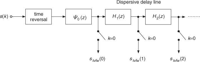
Suppose that each frequency-dependent delay element in the structure of Figure 11.5 has its own phase characteristics θk(ω) and suppose that we remove the scaling filter. Accordingly, the outputs of the structure are the sequences
![]()
with ψ0(k) = δ(k), obtained by convolving the impulse responses am(k) of the allpass filters
![]()
Hence the z-transforms of the sequences ψn(k) are
![]()
and their DTFT is
![]()
where
![]()
is the sign-reversed cumulative phase of the first n delay elements. By multiplying each signal sample s(n) by the corresponding sequence φn(k) we obtain the signal
whose DTFT is
Note that this is an important generalization of (11.3) in which the phase terms are not integer multiples of each other. In the special case where all the delays are equal we have θk(ω) = θ(ω) and Θn(ω) = nθ(ω). If we suppose that the delays are equal in runs of N, then signals of finite length N, supported on the intervals (r − 1)N, ..., rN − 1 are frequency warped according to distinct characteristics. For the same reason, signal samples falling in these intervals are differently warped. Portions of the signal falling in two adjacent intervals are warped in a mixed way. More generally, one can have a different delay for each signal sample. This results in a time-varying frequency warping [EC99, EC00]. From a musical point of view one is often interested in slow and oscillatory variations of the Laguerre parameter, as we will discuss in Section 11.3. It is possible to derive a computational structure for time-varying warping analogous to that reported in Figure 11.6. This is obtained by considering the sequences ψn(k) whose z-transforms satisfy the following recurrence:
where
![]()
and b0 = 0. This set of sequences plays the same role as the transposed sequences (11.9) in the Laguerre expansion. However, the sequences φn(k) and ψn(k) are not orthogonal, rather, they are biorthogonal, i.e.,
Consequently, our time-varying frequency-warping scheme is not a unitary transform of the signal, hence it does not verify the energy preservation property (11.1). However, one can show that this is a complete representation of signals. Hence the time-varying frequency warping is an effect that can be undone without storing the original signal. The modified structure for computing time-varying frequency warping is reported in Figure 11.12. In order to preserve the same direction of warping as in the fixed parameter Laguerre transform, the sign of the parameter sequence must be reversed, which is equivalent to exchanging the roles of θn(ω) and ![]() . The inverse structure can be derived in terms of a tapped dispersive delay line based on Φn(ω) with the warped signal samples used as tap weights. Next we provide a simple M-file 11.3 implementing the structure of Figure 11.12. The function gives a simple implementation of the variable parameter generalized Laguerre transform.
. The inverse structure can be derived in terms of a tapped dispersive delay line based on Φn(ω) with the warped signal samples used as tap weights. Next we provide a simple M-file 11.3 implementing the structure of Figure 11.12. The function gives a simple implementation of the variable parameter generalized Laguerre transform.
Figure 11.12 Structure for computing time-varying frequency warping via generalized Laguerre transform with variable parameter.
M-file 11.3 lagtbvar.m
function y=lagtbvar(x,b,M)
% Author: G. Evangelista
% computes coefficients y of biorthogonal Laguerre expansion of x
% using variable parameters b(k) where b is a length M array
N=length(x);
yy=x(N:-1:1); % time reverse input
y=zeros(1,M);
yy=filter(1,[1, b(1)],yy); % filter by psi_0(z)
y(1)=yy(N); % retain the last sample only
% filter by H_1(z)(unscaled, b to -b)
yy=filter([0,1],[1, b(2)],yy);
y(2)=yy(N)*(1-b(1)*b(2)); % retain the last sample only and scale
for k=3:M
% filter by H_(k-1)(z)(unscaled, b to -b)
yy=filter([b(k-2),1],[1, b(k)],yy);
y(k)=yy(N)*(1-b(k-1)*b(k)); % retain the last sample only and scale
end
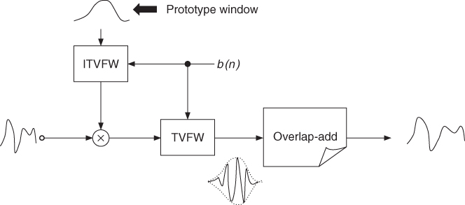
Time-varying frequency warping has a fast approximate algorithm whose block diagram is reported in Figure 11.13. The scheme is similar to the overlap-add method derived for the Laguerre transform and is shown in Figure 11.9. However, due to the time-varying aspect, the inverse time-varying warping of the prototype window must be computed for each input frame.
Figure 11.13 Block diagram of the approximate algorithm for time-varying frequency warping. The blocks TVFW and ITVFW respectively denote time-varying frequency warping and its inverse.
An extension of the vocoder-based frequency-warping algorithm discussed in Section 11.2.5 for handling the time-varying case is available [E08], which works under the assumption that the warping map is constant in each time interval of N samples. Since changes in the warping map are audible only over time intervals larger than 25 ms, this constraint on the update rate is not too severe.